Does the U.S.-China trade war impact the Swedish stock market? : An event study of the impact on the Swedish stock market and which sectors that are the most affected by the trade war

Does the U.S.-China trade war

impact the Swedish stock

market?

An event study of the impact on the Swedish stock market and which sectors that are the most affected by the trade war

MASTER THESIS WITHIN: Business Administration: Finance NUMBER OF CREDITS: ECTS 30

PROGRAMME OF STUDY: Civilekonomprogrammet AUTHOR: Marcus Erlandsson & Sebastian Gappel TUTOR:Fredrik Hansen & Toni Duras

i

Abstract

There is an ongoing trade war between the two largest economies in the world. Since the trade war is still ongoing, few studies have been done to investigate how it affects the global

economy. The purpose of this thesis is to analyze the trade war’s effect on the Swedish stock

market between the 2nd of March 2018 when U.S. president Donald Trump first threatened to

impose tariffs on Chinese imports to the 15th of January 2020 when the phase one deal was

signed. Data is collected from Donald Trump’s official twitter account and by statements from the U.S. and Chinese governments. An event study is then made by using the market model to find abnormal returns for different sectors and stocks on OMXS large cap. The study shows that the sectors react differently to the announcements. Some sectors were not affected at all and others were heavily affected. Telecommunication is a sector that had an average cumulative abnormal return close to zero both when there was positive news and negative news about the trade war. Contrarily, a sector that seems to be highly correlated to the news about the trade war is the Technology sector. Basic Resources is the most affected sector in the study when bad news occurred. From our study, we can conclude that the Swedish stock market is affected by the trade war.

ii

Acknowledgments

The authors of this thesis would like to thank our tutor at Jönköping International Business School, Fredrik Hansen and co-tutor Toni Duras that have provided guidance and inspiration to us throughout this process. We would also like to express an extra thanks to our fellow students that have provided us with important insights during seminars. Without you, this thesis could not have been completed. We are very grateful for your help.

iii

Contents

1. Introduction ...1

1.1 Background ...1 1.2 Timeline ...2 1.3 Problem ...4 1.4 Purpose ...4 1.5 Research Questions ...5 1.6 Delimitations ...5

2. Literature Review ... 6

2.1 Event Studies ...6

2.2 Efficient Market Hypothesis ...7

2.3 Capital asset pricing model ...9

2.4 Market Model ...9

2.5 Cumulative abnormal return ... 10

2.6 Previous research using event studies in finance ... 11

3. Method ... 15

3.1 Scientific approach ... 15 3.2 Model Selection ... 16 3.3 Data ... 18 3.4 Hypothesis ... 20

4. Empirical Findings ... 21

4.1 Findings on event dates ... 22

4.1.1 Bad news ... 22

4.1.2 Good news ... 24

4.1.3 No news ... 26

4.2 Findings on the event study ... 27

4.2.1 Event days ... 27 4.2.2 Estimation Window ... 27 4.3 Descriptive statistics ... 27

5. Analysis ... 29

5.1 Discussion ... 32

6. Conclusions ... 34

6.1 Implications ... 34 6.2 Recommendations ... 35

iv

7. References ... 36

Appendix ... 40

Appendix 1 Companies in the different sectors ... 40

Appendix 2 All shares bad news ... 41

Appendix 3 All Shares Good news ... 43

Appendix 4 Sectors No news... 45

Appendix 5 Event day included when estimating beta and alpha ... 46

v

Definitions

AAR - Average Abnormal Return AR - Abnormal Return

CAAR - Cumulative Average Abnormal Return CAR - Cumulative Abnormal Return

CML - Capital Market Line

CSR - Corporate Social Responsibility EMH - Efficient Market Hypothesis

HARKing - Hypothesizing After the Result are Known MNC - Multinational Corporation

OLS - Ordinary Least Square

OMXSLCPI - OMX Stockholm large cap price index USTR - United States Trade Representative

1

1. Introduction

This thesis will investigate if there has been impact on different Swedish sectors on days where there has been an announcement, a tweet, or news concerning the ongoing trade war between the U.S. and China. Thus far in history, a trade war of this magnitude is uncommon and therefore interesting to study.

The research by Mao and Görg (2019) and Sun, Tao, Yuan and Zhang (2019) shows support that third countries, not the U.S. or China, are indirectly impacted by the tariffs imposed by the U.S. through connections in the supply chains. Mao and Görg (2019) also find that Chinese tariffs on the U.S. imports have less effect on third countries.

1.1 Background

Liu and Woo (2018) argues that there have been three major factors that are underlying and driving the U.S. to act towards a trade war. First is the trade deficit, import-export towards China. Second is that the U.S. argues that China has been involved in stealing technology from American companies. The third concern is a matter of national security as well as having the number one position in the global market.

In 2015 The State Council of China unveiled a large initiative, namely Made in China 2025 (Balderrama & Trejo, 2018), with the goal to make China a manufacturing powerhouse with superior products in various high-tech fields (Hsu, 2018). Another part of the incentive was to strengthen China’s position in the global market by acquiring and investing in foreign

companies involved in new technology primarily in the United States and Europe.

Furthermore, the government in China supports large technological investments with the goal to compete internationally (Balderrama & Trejo, 2018). According to Liu and Woo (2018) one of the first steps of achieving this goal is to become self-sustaining and that 70 percent of parts in a product is produced in China. In a book published a couple of years before the actual trade war, Moosa (2012) argued that an important underlying factor for the trade dispute between the U.S. and China was that the U.S. no longer produces manufacturing products that are being imported from China. This is because the erosion of the industrial base, which tends to be a natural step in the economic evolution. According to Moosa (2012), although this will hurt workers in the short-run, it will be beneficial in the long-run since the workers will find better jobs and benefit from the goods that are being imported from China.

2

In October 2017, Chinese President Xi Jinping stated that China is opening its borders and arguing that the U.S. are doing the opposite. The U.S. argues that China has very high trade barriers and that it is hard for U.S. companies to invest in Chinese firms. One factor is that many firms in different sectors in China needs to be controlled by Chinese investors which means that foreign investors cannot hold more than 49% of the firm (Warner, 2018). Liu and Woo (2018) states that if a firm wants to start distributing their products in China, they might have to open production factories together with a government-linked firm as a joint venture. They also state that this joint venture could potentially become a competitor in other markets. The trade deficit in the U.S. is according to Moosa (2012) an American problem because it is a consequence of too little saving and too much consumption financed by too much debt. What lead to the trade deficit was a lot more spending than saving by the public as well as the private sectors, and that Americans are not producing the goods they intend to consume. Lower amount of savings also decreased the funds that could be used for domestic investments. This led to rising interest rates which made the U.S. attractive for foreign investors. When the saving rate declined in the U.S., the consumption increased. Hence, the U.S. became more dependent on foreign countries (Moosa, 2012).

Another factor of the trade deficit is that the U.S. economy is as of late largely conquered by the financial sector making financial products whilst the Chinese are manufacturing consumer goods and machine tools. Manufacturing employment in the U.S. had its peak in 1978 at 19.3 million workers with the worst deterioration between 2000 (17.2million) and 2010

(11.6million), (Moosa, 2012). As of 2018, the manufacturing employment has increased to 12.7 million workers(BLS, 2019).

1.2 Timeline

We will make an event study based on 13 different tweets, news, announcements, or

happenings concerning the U.S. – China trade war. The timeline section shortly describes the different event dates in the following event study, the first parenthesis is how the news about the event arrived, the third is the OMXS Large cap movement on the specific day and the last is our judgment if it was a negative or a positive event.

→ 2018-03-01(02)- U.S. President Donald Trump threatens to impose tariffs to protect the U.S. steel workers. He states that the U.S. is losing billions of dollars on trade with every trade partner and that trade wars are good for the U.S. (announcement) (Lynch & Paletta, 2018) (-1.97%) (negative)

3

→ 2018-04-03-The U.S. threatens to implement further tariffs on 1333 products worth $50 billion. According to the United States Trade Representative, the reason is China’s unreasonable technology transfer policies to the U.S. economy. (announcement) (USTR, 2018a) (-1.58%) (negative)

→ 2018-04-04-China threatens to retaliate on the auto-, aircraft- and agricultural-sector by raising tariffs over $3 billion in U.S. export. (announcement) (USTR, 2018b) (-0.98%) (negative)

→ 2018-06-15-The U.S. released a revised list on the products from 3rd _{of April, with} plans to impose 25% tariffs on approximately $50 billion worth of Chinese imports that contains industrially significant technologies including those who are related to

“Made in China 2025” in two phases starting 6th _{of July 2018. (announcement)}

(USTR, 2018c) (-1.10%) (negative)

→ 2018-07-20- U.S. President Donald Trump tweets that the U.S. might impose tariffs on all Chinese imports. He further accuses China and the European Union of

manipulating their currencies to remove the U.S. advantages on the market. (Tweet) (-0.16%) (negative)

→ 2018-11-01- U.S. President Donald Trump tweets that the meeting with Chinese president Xi Jinping went well and that trade discussions are moving along nicely. (Tweet) (-0.42%) (positive)

→ 2018-12-01-After a meeting between the presidents, Donald Trump and Xi Jinping in Buenos Aires, they agreed to halt the escalation of tariffs until early March. U.S. President Donald Trump tweeted that the meeting in Argentina went very well and that he had great success dealing with various countries. (Tweet) (0.98%) (positive) → 2019-05-05- U.S. President Donald Trump tweets that China has been paying 25%

tariffs on $50 billion worth of high-tech products and 10% on $200 billion worth of other goods, and that this has helped the U.S. economy a lot. He further tweets that China is trying to renegotiate and that the trade talks are moving too slow. He also writes that the increased tariffs from 10% to 25% will in fact take place on May 10th (Tweet) (-1.29%) (negative)

→ 2019-05-13- China announces that they will retaliate and impose additional tariffs on some of the $60 billion worth of products that was implemented in September 2018. U.S. President Trump tweets that China should not do this, and that things will get worse (Tweet) (-1.58%) (negative)

4

→ 2019-08-01-After a meeting between representatives, U.S. President Donald Trump announced that the U.S. will impose additional 10% tariffs on an additional $300 billion imports from China and that it will take place September 1st_{. Trump tweets that} a trade deal was close months ago, but China decided to re-negotiate the deal before they signed it. (Tweet) (0.78%) (negative)

→ 2019-10-11- U.S. President Donald Trump tweets that things are starting to get better and that there are warmer feelings than in the recent past. He further tweets that he will not impose additional tariffs on Chinese products and that when the deal is signed, it will be a fast process. (Tweet) (1.29%) (positive)

→ 2019-12-12- U.S. President Donald Trump tweets that a deal with China is very close, and that both countries want to get it done. (Tweet) (0.71%) (positive)

→ 2020-01-15- Phase 1 deal is signed. (-0.29%) (positive)

1.3 Problem

The U.S. President Donald Trump, and Chinese President Xi Jinping are making

announcements and implementations that threatens free trade and therefore the global market. When two of the largest economies in the world have a trade war of this magnitude, other countries are heavily affected as well. How does the trade war affect the Swedish stock market and is it the case that one or more sectors is more affected than others? The trade war between the U.S. and China is an ongoing process and therefore there have been no previous investigation on how the trade war is affecting the Swedish stock market. Even though the trade war is in an early stage for evaluation purposes, the findings in this thesis could potentially be even more important and give an understanding for which stocks and sectors that are mostly affected by the trade war so far. A large growing body of literature shows that the stock market is more volatile when political events occur (Chan & John Wei, 1996).

According to Niederhoffer (1971), events impact stock prices and the stock market seem to

overreact to bad news.

1.4 Purpose

The purpose of this thesis is to provide an analysis of the ongoing trade war between U.S. and China and its effects on companies and sectors on the Swedish stock market. Are there any differences between different sectors and companies in abnormal returns? There could potentially be some valuable information for private investors to take into consideration from this analysis. For instance, if one specific sector is not impacted at all (or is less impacted) it could be a more attractive investment if the ongoing trade war escalates further.

5

1.5 Research Questions

The following research questions will be considered in the study: 1. Do the events in the timeline affect the stock market? 2. Are there differences in abnormal returns between sectors? 3. Are there differences in abnormal returns between stocks?

1.6 Delimitations

This thesis will limit its data to OMX Stockholm large cap to avoid the possibility of

involving stocks that are too infrequently traded, since stocks with a low trading volume have a beta that is 10-20% larger than unadjusted estimates according to Scholes and Williams (1977). The data that is being used will be limited to 13 selected dates. These dates have been selected the first time an announcement is being made by representatives from the two

countries, U.S. President Donald Trump, or Chinese President Xi Jinping. To get a fair

judgement of the effects on different companies, it would be optimal to have the same number of event days. Hence, companies that have been listed on the stock market after our first event day or companies that for some reason does not have data for all the event days, will be excluded from our calculations. The language barrier prevents us from looking into Chinese reports about the trade war, which is why we will focus on English announcements and news.

6

2. Literature Review

2.1 Event Studies

In a review on event studies, Corrado (2011) stated that event studies were introduced to a broad audience in the 60’s in the accounting and financial area by two groundbreaking papers by Ball and Brown (1968) and Fama et al, (1969). Ball and Brown (1968) investigated stock reactions when annual reports were released. The main purpose of the report from Fama et al, (1969) was to study the process from which individual stocks prices adjust to information (if there are any) that is implicit in a stock split. Prior to their study, stock splits had been associated with a large increase in dividends. However, the authors found that the market understands this and uses the news to re-evaluate the stocks expected returns.

The event study method has developed over the years, but the key aspects can be found in earlier papers. MacKinlay (1997) reports that an event study was done by Dolley (1933) who studied how stock prices reacted to stock splits and refers to other papers as well, which according to Corrado (2011) indicates that by the 60’s, the event study method was commonly used and several studies was published in economic journals such as Myers (1948), Barker (1956), (1957), (1958) and Ashley (1962). Myers (1948) did a similar study to the one that Dolley (1933) made, but used a larger time interval. The study showed that in the short run, a company’s decision to propose a split of the shares is positively viewed by the market. In the 70 cases that were studied, 63 of the companies had a larger increase in their stock prices compared to the companies in the same industry. Barker also studied stock splits in his papers. He stated that even though stock splits and dividends can increase the number of shareholders, the stock splits alone cannot produce lasting gains. He further states that they are not avoiding a double taxation of dividends nor are they customarily designed to conserve cash. Ashely (1962) found that capital values reacts faster to bad news than to good news. However, the author did not have an explanation for this phenomenon. Three other papers that has contributed a lot to the event study method in the financial area is Modigliani and Miller (1958) and Miller and Modigliani (1961), (1963). They presented issues in the capital structure to the financial area which has led more recent researchers to use the event study to address this issue.

Ball and Brown (2019) replicated their study from 1968 and according to the authors, the results continued to show similar findings. They stated that this indicates that their work from 1968 was successful in measuring the relation between accounting earnings and stock returns.

7

Furthermore, abnormal returns can still be calculated on the announcement day. However, there have been some large differences between now and 1968. The authors stated that the reporting lag has shortened a lot in many countries. Ball and Brown (2019) also stated three important factors that undermines the credibility of a study: P-hacking, HARKing and selective publication. P-hacking is when the researchers are altering the choices of research design and model selection until they find a statistically significant p-value. HARKing

(Hypothesizing After the Result are Known) is when the researcher is changing the hypothesis to fit the results, which makes it easier to find a significant result. Selective publication is the fact that papers with insignificant result are rejected in journals. It could either be because the researchers did not submit the paper or that the journal rejected all papers with insignificant results.

The event study method in finance was developed to measure the effects on stock prices caused by an event. It is based on an estimation of a market model for each individual firm and later calculate possible abnormal returns. The assumption is that the abnormal returns should reflect how the stock market is reacting to new information. In order to conduct an event study and identify abnormal returns there are three main assumptions that needs to hold (McWilliams & Siegel, 1997)

• Markets are efficient

• No anticipation of the event

• No other events during the event window that could have affected the stock prices

2.2 Efficient Market Hypothesis

A frequently used paper when discussing market efficiency is the one by Fama (1970). The definition of an efficient market is that prices “fully reflect” all available information. In this paper, Fama (1970) stated that markets are efficient to integrate new information to asset pricing. Also supported by Ball and Brown (1968), that found that the market will adjust to new information as soon as it is available, they conducted an event study on accounting income numbers for firms between 1946 and 1966. Fama (1970) tested three different

hypotheses. First, the weak form tests, which means that an investor cannot get higher returns by looking at previous stock prices. The second, semi-strong tests, which means that new information is incorporated into the stock price efficiently. Fama (1991) changed the title semi-strong tests to event studies. The last one, strong form tests, means that no investor have a monopolistic access to any information that could be relevant for stock prices. The author

8

showed that the first and the second hypotheses holds, whereas the third is assumed to hold since it is illegal to trade on some sort of private information. Furthermore, to strengthen his findings, Fama (1970) stated that three conditions need to hold. First, there needs to be enough participants. Second, new information needs to be random and not analyzed by some part earlier. Third, every participant tries to fix the price of the asset as soon as the new information reaches them. He further elaborates that the semi-strong form tests, or event studies (Fama, 1991), where stock prices are assumed to take all available information into account supports the efficient market hypothesis.

Chan and John Wei (1996) studied the impact of political news on the stock market volatility in Hong Kong. To better understand the mechanisms of the stock market volatility and its effects, Chan and John Wei (1996) analyzed the Sino-British confrontation, which is the case of the British negotiations with China concerning Hong-Kong (Mushkat, 2011). They

suggested that if the volatility on the stock market increased during the Sino-British confrontation, then the price of different securities should reflect the risk that the political event is causing. If not, there would be arbitrage opportunities. To address this issue, the authors studied two types of stocks on the Hong Kong stock market, blue-chip stocks, and red-chip stocks. Blue-chip stocks are probably the most known ones and are listed on the Hang-Seng index and are controlled by either Hong Kong itself or British businessmen. The red-chip stocks are under the Republic of China’s control. They found significant evidence that the red-chip stocks are more volatile during the event day than on a day where there was no political news. The returns were significantly different when bad news occurred. However, the returns were not significantly different when good political news occurred. They further explained that there are signs that indicates that red-chip stocks are considered a safety in troubled times. Finally, they stated that the market tends to overreact to bad news and underreact to good news.

In more recent studies there have been some criticism towards the EMH. Shiller (2003) argued that the modern view on EMH has changed. The thought that the prices of a security fully reflects the information about fundamental values and only have a change in price corresponding to sensible information is outdated. Additionally, he stated that an investor should not view the EMH as completely wrong. However, he suggested that the EMH can lead to a misinterpretation of major events on the stock market. Instead, Shiller (2003) focused on the behavioral factors that affects stock prices. Evidence has showed that crashes in the stock market were based on human weaknesses and a misallocation of resources. He

9

finally suggested that future researchers should focus more on making the reality a part of their financial models.

2.3 Capital asset pricing model

The capital asset pricing model was developed by William F. Sharpe and describes the relationship between risk and return for a combination of risky assets. In equilibrium, the prices of the assets have been adjusted so a rational investor is able to get any point along the capital market line, as can be seen in the graph below (Sharpe, 1964). When investing on the capital market line, the investor cannot receive a higher expected return without receiving an additional amount of risk. To define the market equilibrium, one need to make two

assumptions. First, one need to assume a common interest rate and that every investor can borrow funds on equal terms. The second assumption is that investors are assumed to have the same expectations. Sharpe (1964) states that these assumptions are unrealistic. However, he further explained that the purpose of the article is not to test the realism of these assumptions and that it is far from clear that they should be rejected. Friedman (1953), stated that complete realism is unattainable and that the question if a theory is reliable or not can only be settled if the predictions are good enough for the purpose and if it is better than predictions from other theories.

Perold (2004) discussed three implications that arises with the capital asset pricing model. First, he argued that possibly the most eye-catching aspect of the capital asset pricing model is what the expected return of a security is not dependent on. The expected return of a security is not dependent on the alone risk. A security with a high beta tends to have a high stand-alone risk, however, that is not necessarily always the case. Hence, as the author stated: “a security with a high stand-alone risk will only have a high expected return to the degree that its risk is derived from its sensitivity to the broad stock market”. Second, the beta of a security measures the amount of risk that cannot be diversified away. Perold (2004) also argued that it is important to remember that the entire stand-alone risk is not priced into the securities expected return, only the part that is correlated with the market portfolio. Third, since the estimations of a security’s expected returns are not based on growth rate of future cash flows, it requires a deep analysis of the firm and the ability to estimate future cash flows.

2.4 Market Model

There have been many various methods used to measure the affects that an event causes on the stock market (Brown & Warner, 1985). A model that has been frequently used is the

10

Market Model. Fama (1998) suggested that the market model is an appropriate model to use when measuring the effects of a press release on the stock market. Cable and Holland (1999) conducted a study based on 30 UK companies where they compared the market model with the capital asset pricing model and concludes that the market model outperforms the capital asset pricing model in most aspects. The study comparison was made by comparing the probability levels at which the two models would be rejected against the general model, from which the CAPM-model and the market model derived from.

The market model is assuming a linear relationship between a security and a market index. The constant and the beta value are calculated by using ordinary least squares (OLS)

estimates from the regression of every firm’s daily stock return. The returns from the market model are the normal returns on a day where an event would not occur. The difference between the normal returns and the actual return is referred to the abnormal return (Mackinlay, 1997).

𝑅

𝑖𝑡

= 𝛼

𝑖

+ 𝛽

𝑖

𝑅

𝑚𝑡

+ 𝜀

𝑖𝑡 (1)

Where Rit is the return on an individual security at a certain point in time, Rmt is the market return, αi is the average rate of return in a period with a zero-market return and βi,is a measure of how sensitive the individual stock is in relation to the market index.

ε

i is the part of the

individual securities return that is a result from an event.The abnormal return is the disturbance factor of the market model and is calculated out of sample.

𝐴𝑅

_𝑖𝑡

= 𝑅

_𝑖𝑡

− 𝛼

_𝑖

− 𝛽

_𝑖

𝑅

_𝑚𝑡

(2) The formula above is used to calculate abnormal return, where ARit is the abnormal return. Rit is the return of the specific firm on a given day, Rmt is the market return the same day, αi is the constant term for the firm, and βi is the slope (beta) of the stock.

Scholes and Williams (1977) developed a consistent estimator of beta in the presence of nontrading. They present evidence that nontrading-adjusted securities that have a low trading volume have a beta that is 10-20 percent larger than unadjusted estimates. However, this problem is close to irrelevant for securities that are frequently traded.

2.5 Cumulative abnormal return

A problem that can arise when using a single day abnormal return is the leakage of information. If a small number of people have knowledge concerning an event before the

11

public has access to the same information, the stock price might be affected. The abnormal return on that event day would then be affected which is why only one event day is not enough to analyze. When using multiple event days, the concept of cumulative abnormal return (CAR) is more suitable to use. CAR is defined as the sum of all abnormal returns over the period that is being analyzed. Given the null distribution of abnormal return and CAR, a test of the null hypothesis can be constructed with the assumption that there is no clustering. This means that there should not be any overlaps in the event windows of the including securities (Mackinlay, 1997).

𝐶𝐴𝑅

_𝑖

= ∑𝐴𝑅

_𝑖𝑡

(3) MacKinlay (1997) further explains that if there are overlapping event windows, the

covariances between the various abnormal returns will not be zero. He suggests two approaches that can be used when facing overlapping event windows. First, the abnormal returns can be summed into a portfolio by using a security level analysis. When using this approach one can use cross correlation of the abnormal returns. Second, one can analyze the abnormal returns without using the CAR. This is often the appropriate alternative when dealing with total clustering, which means that several firms has an event day on the same day. The standard approach is to perform a multivariate regression analysis and using a dummy variable for the event day. The advantage with this approach compared to the last one is that it can be applicable when there are firms with both positive and negative abnormal returns.

2.6 Previous research using event studies in finance

Niederhoffer (1971) was one of the initiators of studying the effects that events have on the stock market. His source of information was headlines in the New York Times, where he analyzed how the stock market reacted to political events, world events, and crisis. He found results that showed strong tendency that the events impact stock prices. However, he did not statistically test the significance of the results due to a small sample size. Furthermore, he also states that some events in the newspaper may have happened months prior to the day they were published. Hence, any result that are based on such definition has no significance. He pointed out that a good headline is usually followed by another good headline, and a bad headline is usually followed by a bad headline. Thus, the day after the event, stock prices tend to move in the same direction as in the event day, whereas in day 2-5 after a bad event, stock prices tends to increase. Thus, the stock market seems to overreact to bad news. He further stated that the event days must be carefully selected. The event could potentially have been

12

announced before the event day. In those cases, the results have no predictive significance. Bremer and Sweeney (1991) had similar findings which showed significant results that extreme negative returns on a stock on average are followed by higher than average returns. Even though the cumulative excess return various over periods, the result were still

statistically significant for every sub-period.

Brown and Warner (1985) used simulation of daily data and examined how daily stock returns, their characteristics, and how an event has an impact on a company's share price. They compared different methods and how well they could identify abnormal returns by randomly selecting 50 securities on various event dates. The market model was the one that found abnormal returns most of the times, slightly outperforming the mean adjusted returns and market adjusted returns. They found that using daily data generally present few obstacles. Furthermore, they stated that methodologies based on the ordinary least square (OLS) market model and using standard parametric in the test are well specified. They also found

correlations between the theoretical part of the model and the empirical part of the model, using a few simple assumptions.

A more recent event study was conducted by Godfrey et al (2009). They investigated whether shareholders are beneficial from CSR activities after a firm has faced a bad event by

examining stakeholder characteristics, firm-specific characteristics, and even-specific

characteristics. In their test, they had 178 samples of legal or regulatory actions against firms between 1993-2003. They wanted to limit their sample size. Furthermore, they aimed to have a large event window, which for them was one day prior to the event day and the event day, to capture the different events. Furthermore, they performed a regression analysis on their

selected stock returns against a market index for a 120-day estimation period. From the regression analysis, they calculated the abnormal return using the market model. They found results that only the event-specific characteristics of a firm indicated an impact on shareholder value.

They found that CSR-activities, especially those who are directed towards secondary

stakeholders, could potentially create value for shareholders following a negative event. The value that the manager is creating by engaging in CSR activities have a similar function as an insurance protection.

Turning to an article review on event studies, McWilliams and Siegel (1997) summarized 29 event studies between 1986-1995 in top management journals, replicated 3 of them, and then

13

analyzed their assumptions when calculating abnormal returns. They criticized many of the journals that used a very long event window and discussed the difficulty with isolating the events when using a large event window. Hence, the event window should be as short as possible to assure that one has control over the confounding effects. It should be long enough to measure the effects of the event. Therefore, they recommended future studies to have a very short event window, 1-2 days. If the event is unanticipated, they recommended using a 1-day event window. In their review they further elaborated that some studies that use long event windows can be due to the effects of the events not being priced into the stock

immediately which violated the EMH. Brown and Warner (1985) have similar findings where they stated that the power of the event test is stronger using a 1-day event window, rather than a –5 to 5 intervals. McWilliams and Siegel (1997) showed that 18 out of the 29 studies

checked for confounding effects.

To avoid the possibility for insider trading, which is one of the assumptions that need to hold when doing an event study, Klassen (1996) suggested removing 10 days prior to the event day. The estimation period prior to the event day varies between earlier studies. Brown and Warner (1985) uses a 239-day estimation period, MacKinlay (1997) and Corhay and Tourani Rad (1996), suggested using a 120-day event estimation window. Peterson (1989) stated that a normal time span to use as an estimation period when using daily returns is 100 to 300 trading days.

There are more aspects to consider when conducting event studies. Foster (1980) discussed five different ways to approach the problem with confounding effects. First, to divide the firms in the sample into different categories such as dividends and earnings. The researcher could then analyze the effects on the various categories. However, this approach is only a reasonable approach if the population is large or if there are few confounding events to analyze. Second, remove firms that are experiencing confounding events. This approach is feasible only if the event window is relatively short. Third, still have the number of firms intact but remove a certain time period from the estimation window. The benefit with this approach is that it keeps more observations than alternative two. A potential problem is to decide how many days to delete from the event window. Fourth, retain all the firms in the sample and try to measure the capital market effect of other events then remove that estimation from the return. Fifth, retain all firms in the sample and ignore the confounding effects and assume they are not significant.

14

Sun et al. (2019) studied the U.S.-China trade war and how it affected the Japanese stock market by analyzing quarterly data on Japanese MNCs affiliates as well as stock price data. They found that affiliates that had a high exposure towards the U.S did have a decrease in sales since the start of the trade war. Furthermore, they found that companies that had a large exposure towards U.S.-China trade faced a decrease in stock prices from the 22nd of March 2018 when U.S. President Donald Trump made his announcement about imposing tariffs on Chinese imports. The authors states that this provides insights on how global value chains are spreading trade shocks. The impact on the affiliates strengthens if they are more involved in the global value chain of the MNCs. Hence, they conclude that the effects of the trade war are affecting third countries as well.

15

3. Method

Under this section we will explain the empirical methodology that is being used in our paper. We will first describe our scientific approach and then move on to the model that we have applied on our events. Thereafter, we will present how we will construct our event study, and finally how we have identified our events. In our study it is important to take the ethical aspects that Ball and Brown (2019) presented into consideration. We will not change the model selection for the purpose of finding a statistically significant result, nor will we change the hypothesis to fit the result.

3.1 Scientific approach

A decision that needs to be made when it comes to the scientific approach of a study is if a natural science model can be applied. There are three different philosophical positions

according to Bryman (2012), positivism, realism and interpretivism. The first is a position that advocates that natural sciences can be applied to social ones. Both deductive and inductive methods can be used. The second position is realism, which shares two beliefs with

positivism. First, the natural and social science should and can be applied when collecting data. Second, there is a reality that is different from how the researcher describes it. There are two different forms of realism, the empirical one and the critical one. The empirical one assumes that reality of the natural order can be understood and the critical one assumes that reality only can be understood if one identifies structures that generates these orders. Interpretivism is the contrary to positivism, it requires a strategy that separates the two sciences and that recognize that social sciences are essentially different to natural sciences. When conducting a social research, one need to choose either a deductive approach or an inductive approach. Bryman (2012) further explains that a deductive theory is a view of the relationship between a theory and the social research. From what is known about a certain topic, the researcher constructs a hypothesis that should be empirical examined. The researcher needs to describe how data will be collected in relation to the constructed

hypothesis. However, in an inductive approach the researcher makes his/her conclusions out of observations. Hence, the main difference between the two approaches is that in the deductive approach the theory come first and is followed by observations/findings. In the inductive approach the observations and findings come first and then followed by a theory. It is common to distinguish between two research approaches, the quantitative approach, and the qualitative approach. The quantitative research approach is comprised of sampling and

16

collecting numerical data with a positivism approach. It is according to Bryman (2012) a deductive method where one tests a hypothesis. On the other hand, a qualitative research method takes an interpretivism approach that focuses on interpreting words instead of

numbers. The qualitative research takes on an inductive method with the aim of developing a theory opposite to the quantitative that aims at testing a theory.

In this thesis, we will use a deductive approach and the philosophical position that will be chosen is the positivistic one. The hypothesis will be based on existing theories and then be the baseline for the process of retrieving data. Thereafter, the hypothesis will be tested.

3.2 Model Selection

We are going to assume that the market is efficient, since the purpose of this paper is not to question the efficient market hypothesis but to study the trade war’s effect on the Swedish stock market. Furthermore, we are studying momentary effects and are therefore indirectly assuming EMH. There have been various methods, such as the Capital Asset Pricing Model, used to measure the effects an event causes on the stock market. However, the most used model to find abnormal returns seem to be to use the market model, which is why we will use it in this paper. Furthermore, the model has been suggested by several researchers, Fama (1998) and Cable (1999). We will use the traditional approach presented by MacKinlay (1997) when constructing our event study, we will also add formula 6 from Brooks (2014). To find the alpha and beta variables, we will do a regression analysis. As Brown and Warner (1985) suggested, methodologies that are based on the OLS market model and uses standard parametric in the test are well specified. Since we will analyze the effects on the stocks on OMX Stockholm large cap, the OMX Stockholm large cap price index is the index we will use as dependent variable to find alpha and beta. As independent variable, we will have the different firms. We will do an estimation of expected return. For any security i the market model is:

𝐸[𝑅

𝑖𝜏

] = 𝛼

𝑖

+ 𝛽

𝑖

𝑅

𝑚𝜏

+ 𝜀

𝑖

(4)

𝐸 (𝜀

_𝑖𝜏

= 0) 𝑣𝑎𝑟(𝜀

_𝑖𝜏

) =

𝜎

2

𝜀

_𝑖𝜏

Riτ andRmτ represent the returns on security i and the market portfolio respectively.

ε

i is the part of the individual securities return that is a result from an event. In the second step,

17

deducting expected returns from the actual stock returns. The expected return can be viewed as “normal” returns.

𝐴𝑅

_𝑖𝜏

= 𝑅

_𝑖𝜏

− 𝛼̂

_𝑖

− 𝛽̂

_𝑖

𝑅

_𝑚𝜏

(5)

ARit is the abnormal return (the disturbance term of the market model on an out of sample basis). In step three, we will do a test statistic by dividing the abnormal returns by its standard error, which follows a normal distribution. SARit is the standardized abnormal return (Brooks,

2014). It is the test statistic for every firm i and for every event day τ that is included in our event study. We will test for three different confidence levels, 0.1, 0.05 and 0,01.

𝑆𝐴̂𝑅

_𝑖𝜏

=

𝐴𝑅̂𝑖𝜏

[𝜎̂ (𝐴𝑅2

𝑖𝜏)]

1/2

~𝑁(0,1)

(6) In the fourth step, equation (7), we will aggregate the abnormal returns into CAR to get the total effect that the trade war has had on each company. This is necessary when measuring the total effects on multiple events.

𝐶𝐴𝑅

̂ (𝜏

_{𝑖 1}

, 𝜏

₂

) = ∑

𝜏2

𝐴𝑅

̂

_𝑖𝜏

𝜏=𝜏1 (7)

Where CAR follows a normal distribution, CARi (τ1,τ2) ~ N(0,σ2i(τ1,τ2)). In the fifth step, equation (8), we will sum up the individual stock’s and sector’s abnormal returns on every day τ and then divide it with the number of event days to get the average abnormal return. For

n number of events, the following formula will be used:

𝐴𝑅

_𝑖

=

1

𝑁

∑

𝐴𝑅

̂

𝑖𝜏 𝑁

𝑖=1

(8)

In the following step, equation (9), we will aggregate the abnormal returns over the entire event window with the same method as in formula five. To calculate cumulative average abnormal return (CAAR) for every stock and sector, the following formula will be used:

𝐶𝐴𝑅

_𝑖

(𝜏

₁

, 𝜏

₂

) = ∑

𝜏2

𝐴𝑅

_𝜏

𝜏=𝜏₁

(9)

In the final equation, we have replicated the t-test from equation 6, but used the AAR. This is used to perform a t-test on each individual date for every sector.

𝑆𝐴𝑅

̅̅̅̅̅̅

_𝑖𝜏

=

𝐴𝑅𝑖𝜏

[𝜎̅̅̅̅(𝐴𝑅2 𝑖𝜏)]

18

3.3 Data

The estimation period prior to the event day varies between earlier studies. Brown and Warner (1985) uses a 239-day estimation period, MacKinlay (1997) and Corhay and Tourani Rad (1996), suggest using a 120-day event estimation window. Peterson (1989) states that a normal time span to use as an estimation period when using daily returns is 100 to 300 trading days. Since more recent research seems to use a shorter estimation window, we are going to use a 120-day estimation window as MacKinlay (1997) suggested which is shown in Figure 1. To reduce the potential problem of overlapping event days we will use one day as our event window. If the stock market is open during the announcement, we will use the same day and if it is not open, we will use the following day. In our dataset there will not be a problem with low trade volume which could be a potential problem when calculating beta of the stocks according to Scholes and Williams (1977). The reason for this is that we will use the large cap list on the Swedish stock market (OMXSLCPI).

Figure 1. Parameter estimation and event day

According to MacKinlay (1997), the event day is generally not included in the estimation window to avoid influencing the performance estimators. Thus, we will exclude the event day in our estimation window. As Klassen (1996) pointed out, insider trading is a common factor that need to be taken into consideration when constructing an event study. Hence, to avoid the risk of insider trading, we will remove 10 days prior to the event day in our estimation

window, which was also suggested by Klassen (1996). The removal of 10 days can be seen in Figure 1. We will retrieve daily data on the large cap list on the Swedish stock market from Nasdaqomxnordic.com.

As previously mentioned, there are different ways to approach the confounding effects. Foster (1980) suggested five approaches to deal with this issue. Since our event window is short (one day), the most appropriate approach to choose seem to be to either remove that specific return that a firm faces that day or to ignore the confounding effects. However, as Foster (1980) mentioned, a difficulty with removing days from our estimation window is to choose the right

19

days to remove. Since we have a short event window and many observations, we are assuming that the confounding effects are not significant. Although, we are aware that the results may differ if we would choose another approach.

We will adjust the daily returns for dividends and for when spin off happens since it would affect our beta for each individual stock. To do this, we need to find what the individual company distributed to the shareholders during the years that we are analyzing. Furthermore, we intend to show the Cumulative Abnormal Return (CAR) on individual stocks and

Cumulative average abnormal returns (CAAR) for sectors. To get an objective perspective of the sorting into sectors we will use nasdaqomxnordic.com and their classification of stocks. The classification of the stock into different sectors can be seen in Appendix 1.

Inclusion criteria:

• OMXLC (Stockholm large cap list) • Have data for all event days

• Included in a sector with at least 2 companies

The companies that will be removed are Arion, Arjo, Epiroc, EQT, Net Entertainment Group, Nyfosa, Traton and Veoneer. None of these companies are one of the largest companies on the Swedish stock market. Therefore, the effect on the index will be relatively small which is why we will not adjust the market index after removing these companies. Sectors that only have one company will not be analyzed since it is difficult to make conclusions for an entire sector if the sector only has one company. Companies (sectors) removed from the study since they are the only ones in a sector are Autoliv (Automobiles and Parts), Hexpol (Chemicals), Modern Times Group (Media), Lundin Petroleum (Oil and Gas). This thesis will not go into the details of the different tariffs and draw conclusion whether or not it should affect different companies on the Swedish stock market.

The event days that will be used in this thesis are the first time an event is announced such as new tariffs, news of the ongoing talks between China and the U.S. as well as easing on tariffs. We will identify the events by going through Donald Trump’s twitter account, USTR or a newspaper reporting on the trade war. These news will be collected from sources in English. We are assuming that the market has adapted to the news when the implementations occur, which is why we have solely selected dates when the different events was first announced. The different events will be categorized as “good news” or “bad news” to investigate if they have a significant impact on the Swedish stock market. We will consider good news to be for

20

example easing of tariffs, positive meetings, and the actual signing of deals. Bad news could be threats about increasing tariffs or the number of products involved in the tariffs. The procedure of selecting an event can be seen in the Appendix 6.

We will also make a robustness test by using the exact same procedure on 10 days when there has been no news about the trade war and see if we can draw more reliable conclusions on the impact of the announcements or tweets.

We will check if there are overlapping events, where the previous event is included in the estimation window for the next event and if it has a significant impact on the abnormal return. To check the impact, we will erase the previous event days, calculate a new estimation

window for each date in our timeline and then compare the results.

3.4 Hypothesis

• There is no average abnormal return for the different sectors when bad news occurs • There is no average abnormal return for the different sectors when good news occurs • There is no abnormal return for the different stocks when bad news occurs

21

4. Empirical Findings

In the empirical findings chapter, we will present our findings on how the Swedish stock market was affected by the U.S.-China trade war. Furthermore, we are testing the null

hypothesis that the events should have zero impact on the performance of Swedish stocks and sectors on OMX Stockholm large cap. We will investigate the data and test for statistically significant results as well as analyzing the abnormal returns. This hypothesis is not rejected if we do not find any significant abnormal returns. However, if we find abnormal returns on the event days that are significant, we will reject the null hypothesis.

Figure 2. Event dates in the study, short version of the timeline

2018-03-01(02)- U.S. President Donald Trump threatens to impose tariffs to protect the U.S. steel workers. (-1.97%) (-)

2018-04-03-The U.S. threatens to implement further tariffs on 1333 products worth $50 billion. (-1.58%) (-)

2018-04-04-China threatens to retaliate by raising tariffs over $3 billion in U.S. export. (-0.98%) (-) 2018-06-15-The U.S. Released revised list on 3rd _{of April products. (-1.10%) (-)}

2018-07-20- Tweet that the U.S. might impose tariffs on all Chinese imports. (-0.16%) (-) 2018-11-01- Tweet that the meeting with Chinese president Xi Jinping went well and that trade discussions are moving along nicely. (-0.42%) (+)

2018-12-01-After a meeting between the presidents, Donald Trump and Xi Jinping met in Buenos Aires, they agreed to halt the escalation of tariffs until early March. (0.98%) (+)

2019-05-05- Tweet that China is trying to renegotiate and that the trade talks are moving too slow. He also writes that the increased tariffs from 10% to 25% will in fact take place on May 10th_.

(-1.29%) (-)

2019-05-13- China announces that they will retaliate and impose additional tariffs on some of the $60 billion worth of products that was implemented in September 2018. U.S. President Trump tweets that China should not do this, and that things will get worse. (-1.58%) (-)

2019-08-01- Tweet that a trade deal was close months ago, but China decided to re-negotiate the deal before they had signed it. (0.78%) (-)

2019-10-11-Tweet that Trump will not impose additional tariffs on Chinese products and that when the deal is signed, it will be a fast process. (1.29%) (+)

2019-12-12- U.S. President Donald Trump tweets that a deal with China is very close, and that both countries wants to get it done. (0.71%) (+)

22

4.1 Findings on event dates

In the following section, we will discuss how the bad news and the good news from the U.S. and China have affected the companies and sectors on OMXS large cap. We will present the abnormal returns for all sectors as well as the cumulative abnormal returns. In the findings section we will refer to the cumulative abnormal return as CAR, cumulative average abnormal return as CAAR and average abnormal return as AAR for simplicity reasons.

4.1.1 Bad news

In this subheading we have gathered the dates where a negative event or message has occurred such as threats of new tariffs or increased tariffs. Interestingly, 49,72% of the

abnormal returns on all shares investigated were positive even though the news were negative. However, when adding all the companies, the CAR for these dates were -55,26% which implies that the negative abnormal returns exceeds the positive ones. Even though the CAR is that negative, there are no sectors that have a CAR that is significantly different from zero at 90% confidence level on all dates.

When looking at the t-tests, average abnormal return for Basic Resources, there are no dates where the statistical results are significantly different from zero at a 90% confidence level. However, there are 5 out of 8 negative average abnormal returns. Adding these average abnormal returns from all negative news, we get a CAAR of -7.28% which is the most

negatively affected sector. Basic resources had their worst day on the 20th _{of July 2018 where} every company in the sector had a negative abnormal return with an average abnormal return of –4.45% The least negatively affected sector was Health Care, where there was only one date with negative average abnormal return. Moreover, the t-tests on Health Care showed no results where the abnormal return was significant from zero. Moving on to another sector that was negatively affected by the announcements, Technology, also with 5 out of 8 dates with negative average abnormal returns.

Food and beverage go in the opposite direction with a CAAR of 2.15%. We also found one date, 15th of June 2018 where the AAR went positive 0.81 and is significantly different from zero at 99% confidence level.

Financial Services had quite a small spread between the most positive AAR, 0.62% and the most negative, -1.54%. The different dates added up to a CAAR of -1.37%. The least affected sector with a CAAR of -0.42% is Telecommunication.

23

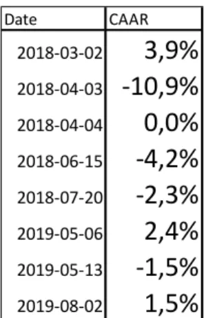
Looking at the CAAR for the various dates, the 3rd of April 2018 stands out amongst the others with a CAR of -10.9%. This was the date when the USTR threatened China to impose further tariffs on $50 billion worth of products. Another date that had mostly negative abnormal returns was June 15th 2018 when the U.S. revised their list from April the same year, the CAAR was negative 4.2%. The OMXS large cap decreased with 1.58% and 1.10% respectively these dates. Out of all sectors, 8 out of 13 had a negative CAAR for dates with negative news and when looking at the CAAR for the different dates, 4 out of 8 dates were

negative. On March 2nd _{2018, most of the sectors had a positive average abnormal return and}

a CAAR of 3.9% whilst the OMXS large cap decreased with 1.97%.

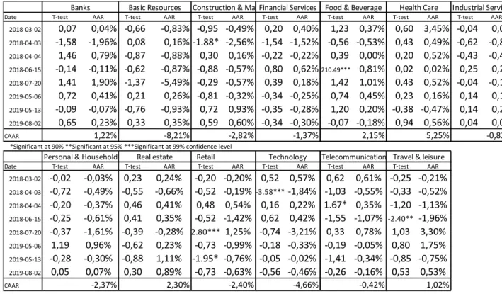
Table 1. Sector reaction on bad news

Date T-test AAR T-test AAR T-test AAR T-test AAR T-test AAR T-test AAR T-test AAR 2018-03-02 0,07 0,04% -0,66 -0,83% -0,95 -0,49% 0,20 0,40% 1,23 0,37% 0,60 3,45% -0,04 0,0% 2018-04-03 -1,58 -1,96% 0,08 0,16% -1.88* -2,56% -1,54 -1,52% -0,56 -0,53% 0,43 0,49% -0,62 -0,8% 2018-04-04 1,46 0,79% -0,87 -0,88% 0,30 0,16% -0,22 -0,22% 0,39 0,00% 0,20 0,52% -0,43 -0,4% 2018-06-15 -0,14 -0,11% -0,62 -0,87% -0,88 -0,57% 0,80 0,62%210.49*** 0,81% 0,02 0,02% 0,25 0,2% 2018-07-20 1,41 1,90% -1,37 -5,49% -0,29 -0,57% 0,39 0,18% 1,42 1,01% 0,43 0,52% -0,04 -0,1% 2019-05-06 0,72 0,41% 0,21 0,26% -0,81 -0,32% -0,34 -0,25% 0,74 0,45% 0,23 0,16% 0,14 0,1% 2019-05-13 -0,09 -0,07% -0,76 -0,93% 0,72 0,93% -0,35 -0,28% 1,20 0,20% -0,38 -0,47% 0,14 0,2% 2019-08-02 0,65 0,23% 0,33 0,35% 0,59 0,60% -0,34 -0,30% -0,07 -0,18% 0,94 0,56% 0,04 0,0% CAAR 1,22% -8,21% -2,82% -1,37% 2,15% 5,25% -0,82%

*Significant at 90% **Significant at 95% ***Significant at 99% confidence level

Personal & Household Goods Retail Telecommunications

Date T-test AAR T-test AAR T-test AAR T-test AAR T-test AAR T-test AAR 2018-03-02 -0,02 -0,03% 0,23 0,24% -0,20 -0,20% 0,52 0,57% 0,62 0,61% -0,25 -0,21% 2018-04-03 -0,72 -0,49% -0,55 -0,66% -0,52 -0,19%-3.58***-1,84% -1,03 -0,55% -0,33 -0,52% 2018-04-04 -0,20 -0,37% 0,46 0,41% 0,48 0,54% 0,16 0,22% 1.67* 0,35% -1,20 -1,13% 2018-06-15 -0,25 -0,61% 0,41 0,35% -0,52 -1,42% 0,62 0,42% -1,55 -1,07% -2.40** -1,96% 2018-07-20 -0,37 -1,61% -0,39 -0,28% 2.80*** 1,25% -0,74 -3,21% 0,33 0,78% 1,03 3,30% 2019-05-06 1,19 0,96% -0,62 0,23% -0,73 -0,99% -0,18 -0,33% -0,19 -0,05% 0,80 1,75% 2019-05-13 -0,28 -0,30% -0,88 1,11% -1.95* -0,76% -0,05 -0,02% -1,41 -0,34% -0,85 -0,75% 2019-08-02 0,05 0,07% 0,30 0,89% -0,73 -0,63% -0,56 -0,46% -0,26 -0,16% 0,53 0,53% CAAR -2,37% 2,30% -2,40% -4,66% -0,42% 1,02%

Travel & leisure Health Care Basic Resources

Real estate Technology

24

Table 2. Cumulative average abnormal return including all sectors on bad news dates

When looking at Appendix 2, which shows individual stocks and their performance over the bad news event dates. There are a few that stands out amongst the others such as Nobia (Personal and Household Goods) -19.47 CAR. SSAB (Basic Resources), with -16.86 CAR. Atlas Copco (Industrial Services and Goods) -11.33 CAR. Boliden (Basic Resources) -9.58 CAR. In the opposite direction we noticed that Elekta (Health Care) had a positive CAR of 13.5 as well as Swedish Match (Personal and Household Goods) 9.22 CAR and Betsson (Travel and Leisure) 8.46 CAR.

4.1.2 Good news

Events that are seen as positive has been the actual signing of the phase-1 deal and news about positive talks between the two presidents. When looking at all shares on the dates when good news was announced, only 42.5% had a positive abnormal return and a CAR of -39.84 %. The sector that was most positively affected by these events was the technology-sector, which had a positive average abnormal return 4 out of 5 times with a CAAR of 4.72%. Another sector that reacted positively to the good news was Basic Resources. The sector had 3 out of 5 dates with positive average abnormal return and a CAAR of 2.88%.

When T-testing AAR on the different sectors when good news occurred, technology was the only sector that was statistically significant from zero at 99% confidence level (2.61). Most of the results on average abnormal return showed no significant return different from zero, however, the banking-sector had a significant result with a 99% confidence level on 2 of the 5 dates with positive news, with a CAAR of 2.35%. Food and beverage had 3 dates that were statistically significant, 2 negative and 1 positive. It has a CAAR of -2.63%.

Date CAAR 2018-03-02

3,9%

2018-04-03

-10,9%

2018-04-04

0,0%

2018-06-15

-4,2%

2018-07-20

-2,3%

2019-05-06

2,4%

2019-05-13

-1,5%

2019-08-02

1,5%

25

The sector that had the worst reaction to the “good news” was the retail sector with a negative average abnormal return for all dates, where two of these being at a 99% significant level.

When looking at the CAAR for all dates, only 2 out of 5 were positive. The 1st of November

2018 had a CAAR of 3.20% across all sectors after U.S. President Donald Trump tweeted that the meeting with Chinese President Xi Jinping went well and that discussions were moving along nicely. The sector that contributed the most on this day were Basic resources with an uprising of 2.97% on average even though the t-test show that the sector is not significantly different from zero. This could imply that there is a large standard deviation amongst the different stocks which will be discussed and analyzed in the analysis section of this work. The

OMXS large cap decreased with 0.42% the 1st _{of November 2018 although there was a}

positive CAAR of 3.20%. The sector that has been the least affected by positive news are Telecommunication, 0.17% CAAR.

Table 3. Sector reaction on good news

Table 4. Cumulative average abnormal return including all sectors on good news dates

Date T-test AAR T-test AAR T-test AAR T-test AAR T-test AAR T-test AAR T-test AAR

2018-11-01 -0,46 -0,28% 0,44 2,42% -0,58 -0,35% -0,23 -0,27%-3.06***-0,50% -0,11 -0,39% -0,18 -0,17% 2018-12-03 -0,62 -0,56% 0,39 1,27% -0,58 -1,07% -0,62 -0,78% 2.07** 1,01% -0,71 -0,88% 0,07 0,14% 2019-10-11 3.23*** 1,68% 0,58 0,75% 0,65 0,56% 0,51 0,66%-2.64***-1,43% -0,11 -0,14% 0,04 0,05% 2019-12-12 7.37*** 1,82% -1,15 -1,49% -0,35 -0,37% 0,12 0,09% -1,03 -1,21% -1,10 -1,55% 0,13 0,16% 2020-01-16 -0,16 -0,32% -0,49 -0,70%-2.19**-0,67% -0,02 -0,01% -0,34 -0,49% -0,13 -0,23% -0,93 -0,63% CAAR 2,35% 2,25% -1,90% -0,30% -2,63% -3,19% -0,46%

*Significant at 90% **Significant at 95% ***Significant at 99% confidence level

Personal & Household Goods Travel & leisure Technology

Date T-test AAR T-test AAR T-test AAR T-test AAR T-test AAR T-test AAR

2018-11-01 0,49 0,74% -0,64 -0,64% -0,31 -0,47% 0,22 0,60% 0,37 1,34% 1,06 1,16% 2018-12-03 -0,32 -0,47% -0,91 -1,04% -0,79 -1,63% -0,05 -0,11% 1.72* 2,12% -0,83 -0,72% 2019-10-11 0,46 0,68% -0,30 -0,44% -1,20 -1,70% 0,03 0,04% 0,81 1,29% -0,37 -0,66% 2019-12-12 0,15 0,46% -0,03 -0,04%-4.99***-1,26% 0,24 0,26% -0,54 -0,14% -1,40 -0,91% 2020-01-16 -0,14 -0,15% 0,39 0,53%-36.93***-0,31%-3.87***-2,61% 0,11 0,11% 0,74 1,30% CAAR 1,27% -1,63% -5,36% -1,82% 4,72% 0,17% Retail

Real estate Telecommunications

Industrial Services & Goods Health Care

Basic Resources

Banks Construction & MaterialsFinancial Services Food & Beverage

Date CAAR 2018-11-01

3,20%

2018-12-03

-2,72%

2019-10-11

1,34%

2019-12-12

-4,17%

2020-01-16

-4,19%

26

Looking at the table in Appendix 3. for all the shares in this study, the ones that had the highest CAR when there was positive news, Lundin Mining (Basic Resources) 16.21% CAR, Boliden (Basic Resources) 8.15% CAR, JM (Real Estate) 8.09% CAR and Billerud Korsnäs (Basic Resources) 7.17% CAR. A share that went the other direction that are also significant from zero when looking at abnormal return at 90% (T-test -1.710) confidence level is Lifco with a CAR of –5.79%. Getinge (Health Care) had no positive abnormal return and ended up on –14.60% CAR. HM did not have a positive day either and –9.04% CAR. Holmen (Basic Resources) also negative all dates and a –8.33% CAR.

4.1.3 No news

The same procedure was made on 10 randomly selected days when no news about the trade war occurred, hence, there was 120 days in the estimation window. This test is seen as a robustness test. The selected dates can be seen in Table 5 below. On these 10 days, a sector that stood out were Food and Beverage with a negative CAAR of 5.16% whilst Health Care as well as Travel and Leisure were in the other end with a positive 5.78% and 5.32% CAAR. Basic resources had the most negative CAAR of all sectors when bad news occurred, and the third most positive CAAR when good news occurred. However, when there was no news at all, the CAAR was -1.21%. Another sector that performed well during the random selected dates was the Personal and Household Goods sector which had a CAAR of +3.15%, and when the bad news occurred the sector had a CAAR of -2.37%. 9 out of 130 t-tests showed a

significant AAR different from zero which is 6.92%.

Table 5. Robustness dates, No news

Dates Returns 3/20/2018 +0.22% 8/28/2018 +0.48% 11/16/2018 +0.75% 1/15/2019 +0.08% 1/31/2019 +0.20% 2/18/2019 +0.13% 5/24/2019 +0.51% 10/24/2019 +0.61% 12/23/2019 +0.14% 1/27/2020 -2.16%

27

4.2 Findings on the event study

In the following sections we will discuss our event study. As previously discussed in the methodology section, we have used an event window of one day. This will decrease the risk of confounding effects which makes it easier to isolate the targeted events.

4.2.1 Event days

We did find both significant and insignificant results for the various sectors. However, most of the events were not significant, and when looking at an event and including all sectors, we did not find any significant results. For the sectors AAR, we found that 10 t-test out of 169 were significantly different from zero at a 99% confidence level which is approximately 5.92%. 13 t-test out of 169 had a significant result different from zero at a 95% confidence level, which is approximately 7.69% of all tests. At a 90% confidence level, 17 out of 169 t-test showed a significant result different from zero, which is approximately 10.06% of all tests.

4.2.2 Estimation Window

In our estimation windows, there was 24 times where an event day is included in the

regression when calculating beta and alpha for the stocks. How it affected the different event days is shown in Appendix 5. As the table shows, the results were very similar and when looking at the CAR for all dates, there was a CAR of -72.12% when the event days were included and a CAR of -71.17% when they were not included. Hence, there was only a 0.95% difference in CAR. The estimation window of 120 days was constructed to be large enough to get a fair beta value but also be small enough to avoid to many overlapping estimation

windows.

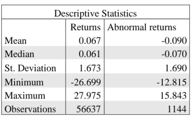
4.3 Descriptive statistics

In the following section the descriptive statistics are presented in Table 6. The “Returns” column describes the statistics for the raw returns on all stocks as well as the index between 2017-08-02 until 2020-01-15. These are returns that are in our estimation windows. For every date there are 92 companies that had data for all dates which adds up to 56637 observations. Looking at Table 6 one can see that there are large discrepancies between the minimum and the maximum returns. For every 13 dates abnormal return there are 88 different samples that had all the inclusion criteria from section 3.3 Data, which adds up to 1144 observations in total. Both the mean and median in the return column are positive whilst they are negative in

28

the abnormal return column. There are also some discrepancies in the abnormal return column when looking at the min and max.

Table 6. Descriptive statistics

Descriptive Statistics

Returns Abnormal returns

Mean 0.067 -0.090 Median 0.061 -0.070 St. Deviation 1.673 1.690 Minimum -26.699 -12.815 Maximum 27.975 15.843 Observations 56637 1144

29

5. Analysis

When looking at the CAAR for all sectors on a specific date, whether it was good news or bad news, we did not find any results that were statistically significantly different from zero. The different sectors did react differently to the various events, and it is therefore impossible to state that the entire Swedish market is reacting in a certain way when there are either good or bad news about the trade war. However, we found large abnormal returns which enables us to see which sectors and stocks that were affected by the trade war.

When looking at the betas of different sectors without taking the abnormal returns into account, health care should have performed better when there was a good announcement, and worse than they did when there was a bad announcement. Thus, the trade war seems to have a smaller effect both positively and negatively on the health care sector. Therefore, it could be viewed as a sector that has less risk if there will be more bad news in this ongoing trade war. However, the complete opposite if good news will dominate. When the bad news occurred,

the sector had a CAAR of +5.25% with only one date with negative AAR, the 13th of March

2019. On the other hand, when good news occurred the sector had a CAAR of -3.19%, ranging from a negative AAR of -0.14% to -1.55%. Not a single t-test was significantly different from zero which could imply that the standard deviation between the different companies was high. Even when removing the two outliers, Elekta when bad news occurred and Getinge when good news occurred, the sector still moved in the same direction but not as extreme as when Getinge and Elekta were included.

The technology sector had mostly positive abnormal returns when there was good news, and mostly negative abnormal returns when there was bad news. This indicates that the

technology sector is more correlated with the news regarding the U.S.-China trade war than other sectors. It was also the only sector that was statistically different from zero. Hence, if one believes that the trade war will continue and bad news will keep coming, the technology sector should probably be avoided. Vice versa, if one believes that the trade war is coming to an end, then it could be a good sector to invest in. However, there could be individual stocks in the technology sector, and other sectors as well, that does not react the same way to the news as the majority of stocks in the same sector. An example of that is in the financial sector where the CAAR was -1.37% for all dates. The CAR of the individual companies was in a span between -3.40 and +1.94 besides Avanza Bank that had a CAR of -8.31%.