Public Services and Migration : A comparison between Swedish rural and urban municipalities

Public Services

and Migration

MASTER THESIS WITHIN: Economics NUMBER OF CREDITS: 30 Credits PROGRAMME OF STUDY: Civilekonom AUTHOR: Louise Fyhr

JÖNKÖPING May 2020

A comparison between Swedish rural and urban

municipalities

i

Master Thesis in Economics

Title: Public Services and Migration - A comparison between Swedish rural and urban municipalities

Author: Louise Fyhr

Tutors: Agostino Manduchi Aleksandar Petreski Date: 2020-05-28

Key terms: public services, migration, rural-urban differences, Tiebout model, rural, Sweden

Abstract

The purpose of this thesis is to examine the relationship between expenditures on local public services and the net migration rate for Swedish urban and rural municipalities. Data from Statistics Sweden over all Swedish municipalities between 2004 and 2014 was used for the empirical analysis. The data also included control variables to control for differences in economic and demographic conditions in the municipalities. The result found using pooled OLS with instrumental variables reveals great differences on the significance of local service expenditure in relation to migration for the two types of municipalities. Childcare was found to be of great significance for rural regions. In contrast, social assistance had a positive association in urban regions while it had a negative insignificant correlation in rural regions. Moreover, culture and education were found to be insignificant in relation to migration for both regions. The results also showed similarities such as elderly care and local taxes were significantly negatively correlated with migration in both type of regions. Overall, the results show that certain local services, such as childcare, are correlated with migration. Nevertheless, economic conditions such as low local taxes, presence of a university campus and having low unemployment are as well of importance to attract residents to both types of municipalities.

ii

Table of Contents

1.

Introduction ... 1

2.

The Swedish Context ... 3

3.

Theoretical Framework ... 5

3.1 The Tiebout Model and Migration ... 5

3.2 Motives for Migration ... 8

3.3 Rural and Urban Differences in Migration ... 9

4.

Methodology ... 10

5.

Results... 18

6.

Robustness Check ... 25

7.

Discussion ... 26

8.

Conclusions... 32

References ... 34

iii

Tables

Table 1 Description of variables ... 12

Table 2 Descriptive statistics for the urban municipalities ... 18

Table 3 Descriptive statistics for the rural municipalities ... 18

Table 4 Regressions for urban municipalities. ... 21

Table 5 Regressions for rural municipalities... 23

Table 1A Definitions and classification of Swedish municipalities... 40

Table 2A List of large city municipalities ... 40

Table 3A List of dense municipalities ... 40

Table 4A List of rural municipalities ... 41

Table 5A Correlation matrix over variable for urban municipalities ... 43

Table 6A Correlation matrix over variable for rural municipalities ... 44

Table 7A Diagnostic tests for urban municipalities ... 45

Table 8A Diagnostic tests for rural municipalities ... 45

Table 9A Regressions with interactions. ... 46

Table 10A Definition and classification of Swedish municipalities ... 47

Table 11A List of large cities and municipalities near large cities ... 47

Table 12A List of medium-sized towns and municipalities ... 48

Table 13A List of rural municipalities ... 48

Table 14A Results from robustness check ... 50

Appendices

Appendix 2 Correlation matrices for urban and rural municipalities ... 43

Appendix 3 Diagnostic tests for econometric models ... 45

Appendix 4 Regressions with interaction terms ... 46

Appendix 5 Definitions and classification of Swedish municipalities (Swedish Association of Local Authorities and Regions)... 47

1

1.

Introduction

Sweden, like the rest of the world, is facing a demographic challenge as the population is getting older together with an increasing urbanisation causing the population to become more concentrated into urban areas. The result of those processes is that the working-age population has become even more unevenly located into urban areas while some rural regions are left with a shortage. This process has come relative far in Sweden by international comparison (SOU, 2015:101) as 85 percent of the Swedish population live in urban regions (Mellander & Bjerke, 2017). In the Swedish context, this poses a problem as many local services such as childcare, education and elderly care are financed by local taxes. Local taxes are strongly connected to the population growth in the municipalities and a smaller and older population results in lower tax incomes and higher cost per user for publicly financed services (SOU, 2015:101). The urbanisation, mainly driven by the working-age population, has left rural municipalities in a situation with lower tax income and greater shares of elderly (Mellander & Bjerke, 2017; SOU, 2015:101). Simultaneously, urban municipalities are faced with problems related to rapid population growth such as housing shortage and a need for great investments (Fjertorp, 2013).

This development has caused Swedish politicians and government agencies to formulate policies on how regions can retain and attract residents. Employment opportunities might not be enough to decrease the out-migration from the most peripheral municipalities, and jobs are as well getting more concentrated into urban areas, which leaves rural areas in a difficult situation. A possible way for regions to attract resident is to offer something which cannot be provided somewhere else. This can include to provide high quality local services in combination with attractive housing, culture and recreational opportunities (SOU, 2015:101). This thesis will examine local services as a potential mean to attract residents to both urban and rural municipalities. The connection between public services and migration has been investigated before, but mostly in the United States with inconclusive results. The result include positive (Bayoh, Irwin, & Haab, 2006; Day, 1992; Friedman, 1981; Nechyba & Strauss, 1998), no significant (Rapaport, 1997) and negative (Quigley, 1985) relationship between local services and migration.

2

It only exists two articles to my knowledge, see (Dahlberg, Eklöf, Fredriksson, & Jofre-Monseny, 2012; Lundberg, 2006a), which have used data from Sweden with the explicit purpose to analyse the connection between migration and local services. This thesis aims at contributing to the literature in two ways. First, the thesis attempts to take a broader approach compared to past literature by using data on local services from all Swedish municipalities and to consider more types of local services. The past literature has tended to only focus on the association between education and migration and has not compared the relative importance of different local services, e.g if school expenditure is of greater importance than childcare expenditure for attract new residents to a community. Second, the previous literature has not considered whether the importance of local services is different between rural and urban regions in Sweden.

Given the past literature, the purpose of this thesis is to fill the gap in the literature by examine the relationship between expenditures on local public services, where local services are defined as childcare, education, elderly care, social assistance, culture and recreational services, and the net migration rate for Swedish urban and rural municipalities, as defined by Growth Analysis, for the period 2004-2014. To conduct the analysis, panel data sets for urban and rural municipalities are constructed based on data from Statistics Sweden.

The purpose has a strong association to current policy making as many rural Swedish municipalities have been and are currently facing economic problems in combination with out-migration of working age residents. A commonly observed solution to the acute issues has been to reduce the expenditure on local services to keep the local budget in balance and/or to raise the local income tax (Swedish Association of Local Authorities and Regions, 2019). Whether or not local services influences the attractiveness of municipalities have implications for policy making in municipalities. A positive association between local services and migration could be a strong argument for maintain or increase spending on local services to attract new residents instead of reducing their spending. The opposite could be an argument for the direct opposite, to continue to reduce expenditures on local services. As the thesis will test different local services and their association with migration, the thesis can also help to point out whether any local service is of greater significance for attracting new residents to urban and rural municipalities.

3

2.

The Swedish Context

To understand the provision of local services in Sweden, the structure of the public sector in Sweden needs to be understood. According to Dahlberg et al. (2012) the public sector in Sweden is large by international comparison. In 2019 the expenditure by the public sector accounts for approximately 20 percent of Swedish GDP (Statistics Sweden, 2020d). The Swedish public sector consist of municipalities and counties (Loughlin, Lidstrom, & Hudson, 2005). Municipalities have the main responsibility for primary and secondary schools, childcare, elderly care and social assistance (Lundberg, 2006b) and counties have the main responsibility for healthcare and public transport (Loughlin et al., 2005). Municipalities have also a great responsibility for recreational and cultural services which include parks, recreational areas, libraries, and leisure-time activities for youths. The main expenditures of municipalities are education, elderly care and childcare, in descending order (Bergström, Dahlberg, & Mörk, 2004). Swedish municipalities have traditionally had great autonomy as local politicians take their own decision regarding the local income tax (Bergström et al., 2004; Dahlberg et al., 2012; Lundberg, 2006b). The local personal income tax is the main source of revenues for municipalities. Based on averages, approximately 60 percent of a municipality’s revenues originate from the local income tax, 20 percent of the revenues comes from other sources (e.g fees paid by residents for certain services) and the last 20 percent consist of governmental grants (Bergström et al., 2004).

The extent of services provided in municipalities will depend on the local tax base. In turn, the tax base will depend on the average income growth and the net migration (Lundberg, 2006b). As net migration rates vary between municipalities and policies on expansion of the local public sector are decided by national political decision, the Swedish government compensate municipalities with small tax bases. If not, poorer municipalities would have to levy unreasonably high taxes to provide the minimum level of basic local services due to the lack of economies of scale. The issue is resolved with the Tax Equalization Grant (TEG), a form of governmental grant. TEG is constructed to ensure it will not exist unreasonable differences in service provision and local taxes for different municipalities (Westerlund & Wyzan, 1995). Municipalities with a greater share of high income residents and smaller economic needs transfer a part of their resources to municipalities with smaller tax bases, in principal this implies a transfer from urban to

4

rural regions (Loughlin et al., 2005). The TEG considers a number of variables including age of residents, social structure, geography and residential structure, which are assumed to affect the production cost of different local services, in order to determine the grant provided to different municipalities (Westerlund & Wyzan, 1995). Moreover, municipalities can undertake debt to finance investments but also handle harsh economic times. Debt can be undertaken to cover budget deficits, but the deficit need to be recovered within three years (Fjertorp, 2013).

In summary, local governments in Sweden have great responsibilities for the provision of local services to their residents. A key issue for municipalities to enable provision of local services is to ensure a sufficiently large tax base, which is closely related to migration. The links between local services and migration are discussed in the next section.

5

3.

Theoretical Framework

This section covers theories of public services and its connection to community choice. The idea of public services connection to migration and community choice is formalised in the Tiebout model. In connection to this theory, some criticism of the model and the past literature, which connect migration and local services provision, is presented. Following this, studies on other motives, except local services, for migration are introduced. Finally, some differences in motives for migration to rural and urban regions are discussed.

3.1 The Tiebout Model and Migration

The connection between migration and public goods or services is formalised by Tiebout (1956). Samuelson (1954) defines public goods as collective consumption goods all enjoy such that each individual’s consumption of the good do not diminish the amount available for the other consumers. In his seminal article, Tiebout (1956) removes the assumption public goods are provided made by a central government, instead he notes that many public goods, e.g childcare and schools (Dahlberg et al, 2012), are provided by local governments. Tiebout argues households chose the community which best satisfy their preferences for local public goods1, instead of staying in a community and try to vote to reach a bundle of public goods which fit their preferences better. The process has later become known as “voting with your feet” (Friedman, 1981). To formalise the model, Tiebout made several assumptions to simplify the analysis. The assumptions include: (1) consumers are fully mobile such they can freely move to a community of their preference, (2) the consumers have perfect information about spending in communities and react to changes in such spending, (3) it exist a large number of communities to choose between, (4) employment opportunities are not considered, (5) the provision of public goods is not subject to economies of scale. The main conclusion by Tiebout (1956) is that households will move freely to the communities which best matches their preferences. The households will shop for public goods and locate in the community which provide the utility maximizing bundle of services and taxes just like private goods are purchased in a market. This process enable the creation of a market of local public goods where

1_{To simplify, I choose to use the term local services instead of the term local public goods or local public} services for most of the thesis.

6

migration become the mean to reach a solution (Mellander, Florida, & Stolarick, 2011) to the non-existent market for local public goods (Dahlberg et al., 2012).

However, the Tiebout model has been subject to much criticism, which is related to the simplified assumptions made. The criticism include households cannot move costless (John, Dowding, & Biggs, 1995; Oates, 1981), the model does not considers employment as obstacles to migration as household need to find suitable employment to migrate (Oates, 1969) and the model does not considers economies of scale which occur due to costs of providing services fall as the population increases (John et al., 1995). Tiebout as well made an implicit assumption that individuals which are dissatisfied with their current bundle of taxes and services will be motivated to move. This implies individuals must have perfect information about communities and be aware of the alternatives. However, this does not hold as individuals do not have perfect information. Even given all the criticism, the Tiebout model has nevertheless become a very influential model (Lowery & Lyons, 1989).

Given the assumptions by Tiebout model, households reveal their preferences for local services by migrating to a community which offers the households the best mix of services, the past literature has considered different public services and its relationship to migration rates. Different jurisdictions have different responsibilities and therefore provide different public services. These differences in responsibility for jurisdictions contribute to previous studies relying on the Tiebout framework have reached different conclusions. Literature from United States includes Friedman (1981) which found a small significant positive effect as more local services attract households to communities. In contrast, Quigley (1985) found a negative effect where more spending on local services repeal residents away from communities which offers more public services relative to other communities. Rapaport (1997) found no significant effect as school expenditure does not affect the location choice of households. Nechyba & Strauss (1998) and Bayoh et al. (2006) both found positive and large effect as expenditure on local services has a significant effect on the location choice of households. Likewise Day (1992), which used data from Canada, found a significant positive effect for a variety of public services and migration.

7

Nordic examples include Dahlberg et al. (2012) which used data from Stockholm, Sweden and found a positive effect for spending on childcare while spending on education and elderly care have no significant effect on migration. Andersson & Carlsen (1997) found a small effect on migration to Norwegian municipalities when testing a variety of public services where education provided the strongest effect on migration. The main conclusion from the past literature is that it is hard to find consensus on whether local services attract households or not to communities. On the other hand, the past literature agrees the results may be hard to translate to different local governments, e.g translate regional level to local government level (Ferguson, Ali, Olfert, & Partridge, 2007) and hence the results may only hold for the specific jurisdiction studied. This may particular be the case for education spending. Dahlberg et al. (2012) argue that due to differences in the school systems, Sweden has likely less variation in spending and quality compared to United States. The choice of methodology also appears to have an impact on the results. Notably both Dahlberg et al. (2012) and Anderson & Carlsen (1997) used two different statistical methods to analyse the data and found slight different results for the data when they both allowed for instrumental variables to mitigate endogeneity. The past literature also agrees the provision of local services is only one reason why households migrate, and numerous of other factors contribute to household’s decision to move.

Moreover, the provision of public goods in one municipality will not only affect the specific municipality, but as well adjacent municipalities. Lundberg (2006a) finds more spending on recreational and cultural activities by one municipality result in lower spending by another neighbouring municipality in Sweden, an example of free-riding. Local tax rates may as well have spillover effects. Westerlund & Wyzan (1995) find short distance migration in dense Swedish municipalities may be partly motivated by lower local tax rates. In dense areas, households are often able to move to a municipality with lower tax rate without changing workplace. Given this assumption, local taxes, are an important factor in the decision to move. In summary, the provision of local services and migration have been studied, but the empirical results do not provide any clear answer whether local services have a significant relation with migration. In the next section other motives for migration is discussed.

8

3.2 Motives for Migration

Local services are only one factor which can contribute to the decision to migrate. According to the human capital model, an individual migrates when the expected future gains exceed the costs of migration. These gains from migration include higher wage level and lower house prices (Rossi, 1955; Sjaastad, 1962). Migration pattern can also be viewed as an interpretation of the Tiebout model. An individual’s preferences for taxes and local services will continually change during its lifetime and this results in migration (Graves & Linneman, 1979), commonly referred to the theory of life-cycle migration (Kulu, Lundholm, & Malmberg, 2018).

A key question in migration has also been whether amenities or employment opportunities is the most important factor when moving (Glaeser, Kolko, & Saiz, 2001; Niedomysl & Clark, 2014). The debate can be summarised into two main fields which either emphasis amenities or work opportunities. The field focusing on amenities and diversity for economic growth has based their ideas on the classical work by Jacobs (1969). The current debate surrounding diversity is mainly driven by Florida (2002a, 2002b) which argues highly educated are attracted by amenities and diversity. By ensure a diverse and vibrant cultural scene, a region can ensure it will attract the most talents individuals. This includes the idea of the city as an entertainment machine, which generates entertainment, nightlife, and culture which in turn contributes to the urban lifestyle (Clark, Lloyd, Wong, & Jain, 2002; Lloyd & Clark, 2001). The other field uses the human capital theory emphasis the link between highly educated and economic development by Romer (1986) and Lucas (1988). The human capital approach focus on highly educated people which are attracted to employment opportunities (Glaeser, 2011; Glaeser, Scheinkman, & Shleifer, 1995). The debate whether amenities or jobs are the most important factor has been studied in Sweden. Highly educated rank work as the most important factor for migration. Moreover, outdoor activities and recreation are also important for those with high incomes (Niedomysl & Hansen, 2010).

Furthermore, migration is subject to spillovers effects. A positive net migration rate in one municipality has a positive effect on the net migration to its adjacent municipalities. An attractive municipality can hence generate more migration to their neighbour (Lundberg, 2006b). In summary, not only the provision of local services can explain

9

migration but also several other factors. These factors can also differ between urban and rural regions, which is presented in the next section.

3.3 Rural and Urban Differences in Migration

Some research concerning motives for migration has taken a closer look on the rural and urban differences in motives. Ferguson et al. (2007) find economic factors, employment rate and income, are the most influential factor for population growth in rural areas. In urban areas the population growth is more related to amenities and are of equal importance compared to economic factors. Local school quality has a positive effect on the migration to rural regions (Barkley, Henry, & Bao, 1998; Marré & Rupasingha, 2020). However, highly educated people also pose a problem for rural areas. Highly educated has more to gain by migrate from rural areas to urban areas due to the wage differences (Sjaastad, 1962) where urban wages are higher (Bjerke & Mellander, 2019). Wage differences are, however, only one factor which influences individuals to move from rural places to urban places. Other motives include a greater range of services and cultural activities (Florida, 2002b; Glaeser, 2011).

Migration to rural regions also depend on the location of the municipality in relation to metropolitan areas. The net migration into rural areas increases the closer the areas is to a regional centre (Aronsson, Lundberg, & Wikström, 2001; Eliasson, Westlund, & Johansson, 2015). Another important rural-urban difference is house prices. Urban rents have in many urban areas growth faster than the wage levels (Gyourko, Mayer, & Sinai, 2013). In Sweden the higher wage earned may not fully compensate for the higher cost of housing in urban areas, and hence individuals are better off financially by live in a rural area with lower house prices and lower wages (Bjerke & Mellander, 2019). Amenities have also an effect on rural migration (Deller, Tsai, Marcouiller, & English, 2001; Graves, 1979) and may partly compensate residents for lower income in rural areas (Roback, 1982). Migration in Sweden is also influenced by fixed endowments such as climate and geography but as well local labour market conditions (Aronsson et al., 2001). In summary, the past literature indicates the preferences for local services and amenities may be different in rural areas compared to urban areas and these differences may be of importance to attract new residents to rural municipalities.

10

4.

Methodology

In this section the data, the definitions of rural and urban municipalities, the variables used in the analysis and the econometric model used in the analysis is presented.

4.1 Data

The data set consist of a balanced panel dataset which covers the period 2004-2014 with 289 municipalities. The variables in the data set are mainly collected from the Statistics Sweden’s data base (see Table 1 for details). The time period is chosen to cover a sufficient period in terms of policy decisions as it generally takes time for political decisions to become implemented and have an impact on the local services provided (Loughlin et al., 2005). Notable is the period cover three general elections (2006, 2010 and 2014) which may have changed the political majorities in the municipalities. The time period does not cover the latest available years (2015-2019) as the migration rates for the most recent years to a large extent consist of asylum seekers (Statistics Sweden, 2020a). Asylum seekers are by law, not free to make a choice on which municipality to settle in (Åslund, 2005). The aim of this thesis is to consider voluntary migration. To include the last years would imply a risk the migration rates reflects involuntary migration by asylum seekers which are allocated to municipalities, therefore the most recent years are excluded from the data set.

Sweden consist of 290 municipalities with the same main responsibilities for local services. However one municipality, Gotland, has extended responsibilities which include healthcare, public transport and regional development (Region Gotland, 2020). Given this, Gotland is excluded from the data set. This has been done previously for the same reason, e.g (Bergström et al., 2004; Lundberg, 2006b). This implies a final dataset of 289 municipalities.

As this thesis is concerned with investigating the association between net migration and local services provide in urban and rural municipalities. The purpose calls for a clear definition of urban and rural municipalities. Swedish authorities have different definitions for various purposes on how to classify municipalities. The used definition is provided by the Growth Analysis. According to their definition municipalities can be divided into three main types based on their population size and degree of urbanisation: large city

11

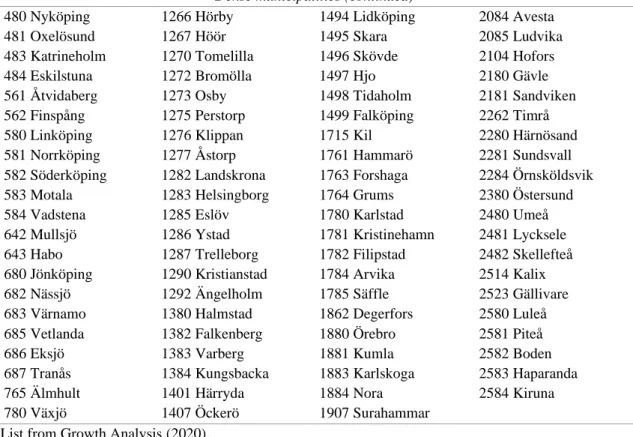
municipalities, dense municipalities and rural municipalities (Growth Analysis, 2020). To simplify, large city municipalities and dense municipalities are merged together to “urban municipalities” and rural municipalities remain “rural municipalities”. The exact definitions for urban and rural municipalities are provided in Appendix 1. Based on my classification, it implies the data set consist of 160 urban municipalities and 129 rural municipalities. Lists with all the municipalities in each group are provided in Appendix 1.

4.2 Variables

In this section the dependent and independent variables are explained and defined. The collected independent variables consist of the variables for the local services, which are the variables of main interest due to the purpose of this thesis, and several control variables which have previously been proven to influence migration. The control variables considered are divided into two groups: economic variables and demographic

variables. Exact definitions and sources of the variables used in the model are presented

12

Table 1 Description of variables

Variable Description

Dependent variable

Net migration ratea _{Defined as}

𝑚𝑖𝑔𝑖,2005−2014= ln(∑2014𝑘=2005𝑛𝑒𝑡𝑖,𝑘+ 𝑝𝑜𝑝𝑖,2005) 𝑝𝑜𝑝⁄ 𝑖,2005 (Lundberg, 2006a)

net is the net migration at year t, the number of in-migrants less

the number of out-migrants from the municipality and pop is the population at year t.

Independent variables Local services

Childcareb _{Childcare expenditure per pupil (0-5 years)}

Educationb _{Education expenditure per pupil (6-15 years)}

Elderly careb _{Elderly care expenditure per senior resident (65+ years)}

Social assistenceb _{Social assistance expenditures per capita}

Culture & recreationb _{Culture and recreational expenditure per capita.}

Economic variables

Tax equalization grantb _{Tax equalization grant per capita.}

Local taxb _{Local income tax in the municipality (%)}

House pricesa _{Average growth of house prices, in per square metre}

Demographic variables

Universityc _{1=university campus. 0= no university campus}

Population densityb _{Population density per square kilometre.}

Unemploymentb _{Share of adult population (20-65 years) which are unemployed}

Key: Data sources for the variables a _{Statistics Sweden (2020c) and the author’s own calculations;} b Statistics Sweden (2020c); c _{Swedish Higher Education Authority (2020). All monetary variables in} Swedish kronor (SEK)

4.2.1 Dependent Variable

Net migration rate

The variable net migration rate captures whether the municipality become more attractive as migrants take the active decision to migrate. The variable net migration rate is different from population growth as it does not include fertility and mortality (Lundberg, 2006b).

4.2.2 Independent Variables

Local services

Local services refer to the variables concerning the expenditure of local public services. Those variables are specified to childcare, education, elderly care, social assistance, and culture and recreation. Childcare refer to the expenditure of taking care of pre-school children. Childcare has been studied previously by Andersson & Carlsen (1997) and Dahlberg et al (2012) which both found that childcare have a significant but modest

13

positive effect on migration to municipalities. The variable education has been extensively studied by previous studies. However, the past literature has reached conflicting conclusions with both positive significant relation on migration, e.g (Bayoh et al., 2006; Nechyba & Strauss, 1998; Rapaport, 1997) and no significant relation to migration, e.g (Rapaport, 1997).

The variables elderly care (the expenditure of provide healthcare to elderly at special homes or in their own homes (Statistics Sweden, 2020c)), and social assistance (the expenditure of provide help to addicts, family counselling, support for vulnerable children and youths, and economic aid to adults (Statistics Sweden, 2020c)), are included. Dahlberg et al. (2012) and Andersson & Carlsen (1997) both found elderly care to be insignificant in relation to migration. This result has been explained by the fact elderly, which consume the most elderly care is, the least mobile in general and therefore the variable is insignificant as it exists too few observations of elderly migrants to find a significant relationship between migration and elderly care. Social assistance has a positive relation to migration, as welfare generosity result in more migration to municipalities due to welfare seeking individuals (Dahlberg & Edmark, 2008; Dahlberg et al., 2012; Åslund, 2005) but can also be a repelling factor for other migrants (Dahlberg et al., 2012). Finally, the variable culture and recreation include the expenditures for libraries, local associations, general cultural arrangements, recreational centres and sports facilities (Statistics Sweden, 2020c). This variable is added to the model as previous literature (Andersson & Carlsen, 1997; Dahlberg et al., 2012) has found expenditure on culture to be positively significant in relation to migration.

For all the variables capturing the quality on different local services, the quality is approximated by using expenditure per potential user for each item. Unfortunately, it does not exist any continuous long-term quality measure of local services in Sweden and therefore the quality of different local services needs to be approximated. Per potential user refer to the group which consume the specific local service. In the case of childcare, the potential user is children aged 0-5, for education, the potential user is children aged 6-15 and for elderly care the potential user is residents aged 65 and above. In contrast, social assistance and culture and recreation are services which are open and made available for all residents, and therefore they are in per capita terms. Per capita

14

expenditure has been used previously for parks and recreational expenditure, e.g Friedman (1981). In contrast, education quality has commonly been approximated by expenditure per pupil, e.g (Nechyba & Strauss, 1998; Quigley,1985). The approach with spending per potential user for a wider variety of services, and not only for education quality, has been used previously by Dahlberg et al. (2012) and Andersson & Carlsen (1997). The method of using per potential user is as well used to mitigate the estimation of the econometric model by decreasing the problem of multicollinearity which occurred when all variables were defined in per capita terms.

Control variables

Economic variables

Economic variables include variables reflecting the economic conditions in the variety of municipality. This include Tax Equalization Grant (TEG), local tax and house prices.

TEG. The TEG per capita is included as previous studies have found that TEG is

negatively correlated with migration, possibly as higher grants indicate lower tax bases and hence lower income levels (Berck, Tano, & Westerlund, 2016; Lundberg, 2006b; Nelson & Wyzan, 1989) while others have found an insignificant effect (Aronsson et al., 2001). Higher TEG may also indicate a declining community with low tax base which repel migrants, especially young migrants. The migrants may be reluctant to pay higher taxes to support the elderly (Berck et al., 2016). Those municipalities which have the largest tax bases receive a negative grant as they pay more per residents than they receive in grants, while those with a smaller tax bases receive positive grants (Loughlin et al., 2005).

Local tax. The variable local tax has been found to have a negative relation with migration

in Sweden as high local taxes repel migrants (Dahlberg et al., 2012; Niedomysl, 2005; Schéele & Andersson, 2018) while other studies have found no significant effect on migration (Niedomysl, 2008). Lower tax rates may also be an incentive for short distance migration in particular (Nelson & Wyzan, 1989).

House prices. In general, higher house prices have a negative effect on migration (Schéele

15

for certain migrants, such as elderly, with less financial resources (Abramsson & Hagberg, 2020). Moreover, higher housing prices do not need to discourage migration as higher prices may reflect higher attractiveness of the city due to urban amenities. Thus, the variety of consumption amenities may compensate for higher housing costs (Clark et al., 2002; Glaeser et al., 2001). Wages are closely related to house prices, as urban areas are often associated with higher wages but also higher house prices as a result of higher wages (Bjerke & Mellander, 2019). Wages have in numerous studies been described as a motivation for migration (Glaeser et al., 2001; Roback, 1982; Westerlund & Wyzan, 1995) as higher wages attract migrants. Moreover, highly educated have more to gain from migration by earning even higher wages by moving to urban regions (Sjaastad, 1962). The variable house price is measured as the growth in house prices instead of average house prices to mitigate multicollinearity in the econometric model.

Demographic variables

The demographic variables include variables reflecting the composition and characteristics of the population. This include the presence of a university, population density and unemployment.

University. The university variable is included due to the establishment of a university

has been found to affect migration rates in Sweden by attracting young individuals (Kulu et al., 2018) and even more notable after the expansion of universities outside of urban regions in Sweden (Andersson, Quigley, & Wilhelmson, 2004). Furthermore, universities attract young individuals which are the most likely to migrate in general (Bjerke & Mellander, 2017).

Population density. The variable population density is included as past studies have found

denser areas to have faster population growth (Glaeser et al., 2001; Lundberg, 2006a; Niedomysl, 2005). High population density contribute to positive agglomeration effects such as knowledge spillovers (Glaeser, 2011) but may also contribute to congestion costs in urban areas which have a negative effect on migration (Buch, Hamann, Niebuhr, & Rossen, 2014). Furthermore, population density can act as a signal for an attractive location due to the possible presence of attractive urban amenities (Berck et al., 2016)

16

Unemployment. Finally, the variable unemployment rate is included as unemployment is

negatively correlated with migration to a municipality (Aronsson et al., 2001; Buch et al., 2014; Eliasson et al., 2015; Niedomysl, 2005) as employment opportunities have been found to be a driver of migration (Hansen & Niedomysl, 2009). The negative relationship with migration may reflect out-migration from the region of the most productive individuals which have the most to gain by moving (Lundberg, 2003).

4.3 Econometric Model

Numerous previous studies within the field of migration, e.g (Andersson & Carlsen, 1997; Andrews & Martin, 2010; Buch et al., 2014) have used longitudinal micro data which has the ability to follow resident’s location choices over several years. As micro data on individual’s migration is not available, the choice of using macro data in the form of panel data should imply sufficient numbers of observations to follow resident’s migration pattern and see tendencies between migration and the independent variables over time. As the data set consist of panel data, the econometric model is based on panel data regression, more specifically pooled Ordinary Least Squares (OLS).

The pooled OLS regression model is given by

𝑁𝑒𝑡 𝑚𝑖𝑔𝑟𝑎𝑡𝑖𝑜𝑛 𝑟𝑎𝑡𝑒_𝑖𝑡= 𝛼 + 𝛽(𝑃𝑢𝑏𝑙𝑖𝑐 𝑠𝑒𝑟𝑣𝑖𝑐𝑒𝑠)_𝑖𝑡+ 𝛾(𝐸𝑐𝑜𝑛𝑜𝑚𝑖𝑐)_𝑖𝑡+ 𝛿(𝐷𝑒𝑚𝑜𝑔𝑟𝑎𝑝ℎ𝑖𝑐)_𝑖𝑡+ 𝜀_𝑖𝑡

The dependent variable is the net migration rate for municipality i in year t. The three groups of independent variables included are: public services, economic variables, and demographic variables. The error term is given by 𝜀_𝑖𝑡.

Given the nature of the data of migration and quality of local services, endogeneity is a potential issue. Quality on local services can in itself depend on the migration to the municipality as a greater population implies more tax revenue and hence more resources can be devote to local services which can be used to increase quality of the services (Andersson & Carlsen, 1997; Dahlberg et al., 2012; Nechyba & Strauss, 1998). In turn the higher quality can then potentially attract even more residents. To handle the endogeneity issue, the instrumental variable (IV) approach of Two-Stage Least Squares (2SLS) is used. The instrumental variables consist of the independent variables lagged by one year. A similar approach of using 2SLS as instrumental variable has been used by Buch et al. (2014).

17

All the specifications are tested for the presence of cross section dependence with the Pesaran cross section dependence test and heteroskedasticity with a panel data heteroscedasticity test.

18

5.

Results

The results section is divided into three different section. First the descriptive statistics, then the correlation analysis and lastly the regression results are presented for urban and rural municipalities, respectively.

5.1 Descriptive Statistics

The descriptive statistics with mean, standard deviation (Std.dev), minimum and maximum is presented below in Table 2 and 3 for urban and rural municipalities.

Table 2. Descriptive statistics for urban municipalities

N=1600, n=160

Variable Mean Std.dev Minimum Maximum

Net migration rate 0.005 0.000 -0.012 0.034

Childcare 77745.23 210.54 38247.05 119733.92

Education 81050.24 243.74 57886.87 127939.07

Elderly care 52672.52 186.35 30813.38 89667.68

Social assistance 3094.67 24.68 702.00 7229.00

Culture & recreation 2337.89 14.19 914.00 4636.05

TEG 6227.18 97.69 -14708.00 16304.00 Local tax 0.211 0.000 0.171 0.233 House prices 0.05 0.00 -0.32 0.52 University 0.24 - 0.00 1.00 Population density 231.31 15.42 1.10 5073.60 Unemployment 0.06 0.00 0.01 0.17

Note: The variable net migration rate and local tax are reported with three digits, and not two digits as the other variables, to being able to highlight the small numbers. The variable university is a dummy variable.

Table 3. Descriptive statistics for rural municipalities

N=1290, n=129

Variable Mean Std.dev Minimum Maximum

Net migration rate 0.001 0.000 -0.023 0.026

Childcare 79732.06 285.53 48355.46 118284.54

Education 90053.94 372.31 61678.89 137368.24

Elderly care 59146.93 265.37 20032.00 99565.88

Social assistance 2693.74 24.73 720.00 7542.00

Culture & recreation 2181.87 17.12 757.00 4497.90

TEG 10963.98 140.61 -3176.00 26982.00 Local tax 0.219 0.000 0.185 0.239 House prices 0.05 0.00 -0.28 0.48 University 0.01 - 0.00 1.00 Population density 18.91 0.66 0.20 176.30 Unemployment 0.07 0.00 0.01 0.17

Note: See notes for Table 2.

For the dependent variable net migration rate, urban regions have a higher mean compared to rural regions. This is further reinforced by comparing the maximum and minimum values where urban regions have higher maximum and lower minimums compared to rural regions. Rural municipalities have a minimum value of 2.3 percent compared to the minimum value of 1.2 percent for urban municipalities. The reverse

19

holds for the maximum values where the urban regions have a maximum of 3.4 percent compared to 2.6 percent for rural municipalities. For local service expenditures, on average the rural municipalities spend more on childcare, education, and elderly care while urban municipalities spend more on social assistance and culture. The rural regions spend more on the most expensive local services, childcare, education, and elderly care, compared to their urban counterparts.

For TEG (Tax Equalization Grant), where a negative value indicates larger tax bases, the urban regions have a much lower minimum. The reverse hold for the maximum values. The observation confirms tax incomes in general are transferred from urban areas to rural areas with lower tax bases. This observation is confirmed by a closer inspection of the data set which show only one rural municipality has negative TEG, all the other regions receive grants. When comparing the averages local taxes, the rural taxes are slightly higher on average compared to the urban taxes with 0.219 compared to 0.211. Furthermore, on average, the growth of house prices is identical with growth of 5 percent for both urban and rural regions. However, the highest growth in prices has occurred in urban regions.

For the variable university, with an average of 0.24 and 0.01 for urban and rural regions respectively, reflect universities are more present in urban regions. The data set show only one rural municipality has a university campus. The population density is substantially higher for the urban municipalities compared to the rural municipalities with over 230 inhabitants per square kilometre compared to approximately 19 inhabitants per kilometre. For the variable unemployment, the descriptive statistics is almost identical, except unemployment on average is 1 percentage point higher in rural regions. In summary, the descriptive statistics show clear differences in migration and the expenditures on local services for urban and rural regions. The descriptive statistics also show differences in economic and demographics conditions which are further explored in the correlation analysis.

5.2 Correlation Analysis

The correlation matrices for the urban and rural municipalities are presented in Appendix 2.

20

In the matrix for urban municipalities net migration rate has a significant positive correlation with childcare, social assistance, university, and population density. The variables elderly care, culture, and recreation, TEG, local tax, and unemployment are significantly negative correlated with net migration rate. Education and house prices are insignificant correlated with net migration.

In the matrix for rural municipalities, net migration rate has a significant positive correlation with the variables childcare and population density. The variables education, elderly care, TEG, local tax, university, and unemployment are significantly negative correlated with net migration rate. Social assistance, culture and recreation, and house prices are insignificant. In general, the correlations between the independent and dependent variables are lower for the rural municipalities compared to the urban municipalities. The results from the correlation analysis is also used for the empirical results in the next section.

5.3 Regression Results

In this section the econometric models for urban and rural municipalities are presented in two tables. Both the tables consist of six specifications where the first three models are pooled OLS models and the latter are pooled OLS models estimated with instrumental variables (2SLS) to account for endogeneity. In all the specifications, the groups of variables, local services, economic variables, and demographic variables, are added stepwise.

In the preliminary modelling, the variables wages and human capital were included in the model as those variables have been identified as factors which influence migration. However, those variables had to be excluded due to the high correlations these variables had with the other variables in the model. In the correlation matrices both urban and rural municipalities, wages and human capital had high correlations (>0.5) with TEG, local taxes and population density. The correlations between human capital and wages were especially high with correlations above 0.7. These high correlations caused severe multicollinearity in the estimated models. The strong association between wages, human capital levels and house prices could be expected given the previous literature on the topic which has emphasised the strong link e.g (Bjerke & Mellander, 2019; Glaeser et al.,

21

2001). Higher human capital results in higher wages which in turn can be capitalised into higher house prices where those with high human capital lives. Given this, wages and human capital had to be excluded in the models.

Table 4. Regressions for urban municipalities. Dependent variable: net migration rate

Variable

Model

Pooled OLS Pooled OLS IV (2SLS)

1 2 3 4 5 6 Constant 6.31e-3_*** (1.17e-3₎ 0.04*** (2.15e-3₎ 0.04*** (2.42e-3₎ 0.01*** (1.44e-3₎ 0.05*** (2.30e-3₎ 0.04*** (2.70e-3₎ Local services Childcare 9.43e-8_*** (1.65e-8₎ 4.58e-8_*** (1.57e-8₎ 3.77e-8_** (1.58e-8₎ 6.50e-8_*** (1.98e-8₎ 1.31e-8 (1.90e-8₎ 5.98e-9 (1.97e-8₎ Education -5.30e-8_*** (1.42e-8₎ -9.01e-9 (1.34e-8₎ 6.49e-9 (1.37e-8₎ -7.68e-8_*** (1.64e-8₎ -2.09e-8 (1.73e-8₎ 2.35e-9 (1.82e-8₎ Elderly care -9.17e-8_***

(1.58e-8₎ -1.13e-8 (1.50e-8₎ -2.81e-8_* (1.58e-8₎ -1.27e-7_*** (1.73e-8₎ -3.93e-8_** (1.68e-8₎ -5.03e-8_*** (1.81e-8₎ Social assistance 7.70e-7_***

(1.07e-7₎ 6.95e-7_*** (9.29e-8₎ 6.81e-7_*** (1.13e-7₎ 1.02-6_e*** (1.17e-7₎ 9.25e-7_*** (1.03e-8₎ 9.89e-7_*** (1.35e-7₎ Culture & recreation -9.04e-7_***

(1.90e-7₎ 1.63e-7 (1.76e-7₎ 1.21e-7 (1.93e-7₎ -8.13e-7_*** (2.14e-7₎ 2.96e-7 (1.93e-7₎ 3.00e-7 (2.19e-7₎ Economic variables TEG 5.72e-8_* (2.94e-8₎ 1.30e-7_*** (3.19e-8₎ 1.66e-8 (3.16e-8₎ 8.67e-8_** (3.57e-8₎ Local tax -0.21*** (0.01) -0.20*** (0.01) -0.21 (0.01) -0.19*** (0.01) House prices 2.23e-3_*

(1.19e-3₎ 2.15e-3_* (1.20e-3₎ 1.00e-3 (4.02e-3₎ 2.50e-3 (4.29e-3₎ Demographic variables University 1.19e-3_*** (2.31e-4₎ 1.01e-3_*** (2.54e-4₎

Population density 1.77e-7

(2.96e-7₎ 1.47e-7 (3.00e-7₎ Unemployment -0.023** (5.42e-3₎ -0.03*** (8.62e-3₎ n 1600 1600 1600 1440 1440 1440 R2 _{0.093 0.273 0.290 0.119 0.309 0.320} Adj. R2 _{0.090 0.269 0.285 0.116 0.305 0.314} F-statistic 32.79*** 74.83*** 58.99*** 34.48*** 80.58*** 59.41***

Note: Robust standard errors in parentheses. The instrumental variables are all the independent variables included in each specification lagged by 1 year. ***p<0.01, **p<0.05, *p<0.1

In Table 4 the first part of the analysis is presented with the regression outputs for urban municipalities. Due to the presence of heteroskedasticity and cross section dependence, see Appendix 3 for details, the models are presented with cross-section weights and robust standard errors. In Model 1, 2 and 3 the signs of the coefficients remain stable, except education, and the only notable change after including more variables is the significance of the variables. In model 1, with only local services, all the variables are significant in

22

relation to net migration rate. In the full model, Model 3, childcare, elderly care, and social assistance are significant among the local services. In contrast the economic variables are all significant and all the demographic variables, except population density are insignificant.

In Model 4, 5 and 6 the instrumental approach is applied. By apply this approach it should be possible to see if it exists any potential issues of endogeneity such that the estimates significance change when considering the endogeneity among the variables. The results in Model 6 remain similar to Model 3 as the coefficients keep their signs. However, childcare becomes insignificant, elderly care becomes more significant, TEG becomes less significant and house prices become insignificant. The result show it exists some endogeneity which affect the significance of the variables, but all the coefficients keep their initial signs. In Model 6, the estimated model explains 31 percent of the variation in the dependent variable.

23

Table 5. Regressions for rural municipalities. Dependent variable: net migration rate

Variable

Model

Pooled OLS Pooled OLS IV (2SLS)

7 8 9 10 11 12 Constant 6.32e-3_*** (1.40e-3₎ 0.03*** (3.95e-3₎ 0.02*** (4.08e-3₎ 6.97e-3_*** (1.696e-3₎ 0.03*** (4.55e-3₎ 0.02*** (4.86e-3₎ Local services Childcare 1.15e-7_*** (2.00e-8₎ 1.12e-7_*** (1.95e-8₎ 1.08e-7_*** (1.93e-8₎ 1.06e-7_*** (2.66e-8₎ 9.80e-8_*** (2.75e-8₎ 8.40e-8_*** (2.92e-8₎ Education -3.97e-8_** (1.61e-8₎ -9.25e-9 (1.63e-8₎ -6.50e-9 (1.62e-8₎ -2.36e-8 (2.07e-8₎ 5.49e-9 (2.20e-8₎ 4.63e-9 (2.25e-8₎ Elderly care -1.75e-7_***

(1.98e-8₎ -9.58e-8_*** (2.28e-8₎ -8.34e-8_*** (2.26e-8₎ -1.96e-7_*** (2.32e-8₎ -9.61e-8_*** (2.81e-8₎ -8.39e-8_*** (2.81e-8₎ Social assistance -2.59e-7

(1.81e-7₎ -1.12e-7 (1.75e-7₎ 7.56e-8 (1.79e-7₎ -3.67e-7_* (2.14e-7₎ -1.82e-7 (2.16e-7₎ -1.29e-7 (2.65e-7₎ Culture & recreation -5.06e-8

(2.60e-7₎ -2.57e-7 (2.60e-7₎ -2.35e-9 (2.60e-7₎ 6.46e-8 (2.91e-7₎ -1.83e-7 (2.98e-7₎ -1.05e-7 (3.10e-7₎ Economic variables TEG -2.99e-8 (4.19e-8₎ 4.63e-8 (4.32e-8₎ -5.00e-8 (4.78e-8₎ -2.15e-8 (4.98e -8₎ Local tax -0.15*** (0.02) -0.11*** (0.02) -0.15*** (0.02) -0.11*** (0.02)

House prices 3.38e-3_**

(1.68e-3₎ 3.87e-3_** (1.66e-3₎ 3.59e-3 (6.86e-3₎ -5.89e-3 (7.49e-3₎ Demographic variables University -5.41e-3_** (2.61e-3₎ -4.32e-3 (2.90e-3₎

Population density 4.32e-5

(6.44e-6₎ 3.81e-5_*** (6.81e-6₎ Unemployment -0.03*** (6.80e-3₎ 3.47e-3 (0.01) n 1290 1290 1290 1161 1161 1161 R2 _{0.092 0.136 0.189 0.089 0.114 0.144} Adj. R2 _{0.089 0.131 0.181 0.084 0.108 0.136} F-statistic 26.24*** 25.27*** 27.01*** 20.97*** 21.40*** 21.14***

Note: Robust standard errors in parentheses. The instrumental variables are all the independent variables included in each specification lagged by 1 year. ***p<0.01, **p<0.05, *p<0.1

In Table 5 the first part of the analysis is presented with the regression outputs for rural municipalities. Like in the case of urban municipalities, the specifications have presence of heteroskedasticity and cross section dependence, see Appendix 3 for details, and therefore all the specifications are presented with cross-section weights and robust standard errors. In Model 7, 8 and 9 the signs of the coefficients remain stable, except social assistance and TEG which both turn positive from negative, and the only thing that changes while including more variables is the significance of the variables. In Model 7, with only local services, all the variables are significant in relation to net migration rate, except social assistance and culture. In the full specification, Model 9, only childcare and elderly care are significant among the local services coefficients. Among the economic

24

variables local tax and house prices are significant and among the demographic variables the presence of a university campus and unemployment are significant in relation to net migration rate.

In Model 10, 11 and 12 an instrumental approach is applied to test for the possible endogeneity in the model. By comparing the results from Model 9 and Model 12 the instrumentation changes the signs of some coefficients, which were not the case for the urban municipalities. Education remains insignificant but changes signs and turn positive, as previous found in the urban sample. TEG remains insignificant but turns negative in relation to migration. Among the previous significant variables found in Model 9 house prices and unemployment turn insignificant and change signs where house prices now have a negative correlation with migration and unemployment has a positive correlation with migration. Furthermore, population density is found to be positively correlated with migration. Population density was insignificant in the urban sample. In the full specification in Model 12, the estimated model explains 13 percent of the variation in the dependent variable. The fit of the model is notable much lower compared to the estimated model, Model 6, for urban municipalities which explains 31 percent of the variation in net migration rate.

Furthermore, a consistency check is performed, se Appendix 4, with interaction terms for all local services to test if the rural-urban differences are statistically significant. This is possible by combine the urban and rural data set and apply a dummy variable to indicate urban regions in the data set. The results show the difference in childcare is statistically significant and hence childcare has significant greater influence on migration to rural regions than urban region. Similarity, education is of greater significance in rural regions, but the interaction term is insignificant. Elderly care is significantly positive indicating elderly care expenditure is of greater importance in urban regions. The same result is also found for social assistance. The interaction term of culture is insignificant but indicate culture and recreation are of greater importance for urban regions relative to rural regions. The test shows the differences in importance of childcare, elderly care and social assistance is significant between urban and rural regions.

25

6.

Robustness Check

In this section a robustness check is carried out to examine the validity of the empirical findings. The past empirical analysis is based on a definition of urban and rural municipalities provided by the Growth Analysis. However, it may be the case the conclusions do not hold once you change the classification of Swedish municipalities. Therefore, the robustness of the findings is tested by using another classification of Swedish municipalities provided by The Swedish Association of Local Authorities and Regions. In their classification they define three main groups of municipalities: large cities and municipalities near large cities, medium-sized towns and municipalities near medium-sized towns and smaller towns/urban areas and rural municipalities. In comparison with the previous used classification, which focus on population in urban regions and the degree of urbanisation, the classification also consider the commuting patterns of the residents (Swedish Association of Local Authorities and Regions, 2020). The exact definitions and full lists on the municipalities included in each group are provided in Appendix 5. The outputs from the regressions are provided in Appendix 6.

For the urban municipalities all the variables which were significant in the original IV model remain significant and with the same sign in Model 17 compared to Model 6 estimated using the same approach. Elderly care, social assistance, local tax, university, and unemployment remains significant under the new definitions. Likewise, for rural municipalities childcare, elderly care, local tax, and population density remain significant and with the same signs compared to Model 12.

However, for both type of regions it also exists differences, education becomes significant for both with positive correlation for urban regions and negative correlation with migration for rural regions. TEG, which was significant for urban municipalities becomes insignificant. The presence of a university campus also becomes significantly positive for rural municipalities. This can be contributed to that the rural sample now include 13 municipalities with universities, compared to in Model 12 which had one municipality with a campus. Therefore, the presence of a university appears to be positively associated with migration for both urban and rural regions. Overall, the main conclusions from the regression models remain valid under the other definition for urban and rural regions and confirm the robustness of the initial empirical findings.

26

7.

Discussion

Given the presence of endogeneity, the discussion will focus on the pooled OLS models with instrumental variables, Model 6 for urban and Model 12 for rural municipalities.

In the result from urban municipalities the coefficients have the expected sign given the previous conducted correlation analysis, except for education and culture which both turn positive in Model 6, even if they were negative in the correlation matrix. The same hold for rural municipalities where the signs of the variables in Model 12 are the same as found in the correlation matrix, except house prices and unemployment which are both positive in the estimated model, were negative in the correlation matrix.

For both urban and rural municipalities, childcare is positively correlated with migration, but is only significant for rural municipalities. The difference between urban and rural regions is also significant. The rural result confirms the previous findings from Norway by Andersson & Carlsen (1997) and from Sweden by Dahlberg et al. (2012) which has found childcare to be significant for migration. The differences in significance between urban and rural regions could be related to distances. As suggested by Westerlund & Wyzan (1995), but in connection to short versus long-distance migration, parents in rural municipality may not have commuting options available which can be used instead of migration to find a suitable childcare facility. Furthermore, Bjerke & Mellander (2017) have found that households are more likely to move from rural areas once they have children, which could be related to the lack of suitable childcare in rural areas. Therefore, childcare becomes much more important in rural areas due to limited commuting alternatives.

Similarly, education was found to be positively correlated with migration for both urban and rural regions. The coefficients where insignificant in both models. The result points towards education may not be of great importance for migration as suggested by Rapaport (1997) and Dahlberg et al. (2012). The results could also be a result of the Swedish education system which emphasis equality, as suggested by Dahlberg et al. (2012), and therefore quality of education is not allowed to vary to much between municipalities. This is as well confirmed by the difference between the regions is insignificant when considering interactions terms. Given this, households do not need to

27

migrate to obtain quality education and education does not become significant in relation to migration.

In contrast, the variable elderly care was found to be significantly negatively associated with migration for both urban and rural municipalities. The difference is also found to be significant between the two types of municipalities. This result diverges from previous results which have found elderly care to be insignificant for migration, e.g (Andersson & Carlsen, 1997; Dahlberg et al., 2012). Possibly the result could reflect expenditure on elderly care act as a signal to potential residents as suggested by Berck et al. (2016). In their study they argue large shares of elderly repel migrants, which mostly consist of young individuals, and signal a declining community which repel new residents. A greater share of elderly may be a proxy for economically depressed locations. More elderly, which require more elderly care, could therefore results in a negative correlation with migration. This could be an explanation for why elderly care is significantly negative in both urban and rural areas and no rural-urban difference exists.

Social assistance was found to have a significant positive correlation with migration in urban regions while it was negative and insignificant for rural regions. Past literature has concluded that greater welfare generosity can attract individuals to certain regions, e.g (Dahlberg et al., 2012; Åslund, 2005). The results could therefore be a sign of welfare seeking in urban regions. In contrast, the negative correlation for rural regions indicate social assistance repel migrants. This is in line with Dahlberg et al. (2012) which argue welfare genorosity may attract certain migrants but also repel other migrants. The found rural-urban difference could possible be due to the limited access to mental healthcare and substance use treatment outside urban areas due to lack of specialised clinics, as

found in an American context (Orsi, Yuma-Guerrero, Sergi, Pena, & Shillington, 2018) which means less users of social assistance, such as drug users, can live in rural areas. This could then make social assistance have a negative relation with migration in rural areas. However, social assistance includes more than just provide care to drug users and the lack of treatment may only be part of the explanation for the rural result.

The variable culture and recreation were found to be insignificant for both urban and rural municipalities but positive for urban and negative for rural regions. The urban results confirm to numerous studies which have found culture and recreation expenditures to be

28

positively associated with migration, e.g (Andersson & Carlsen, 1997; Dahlberg et al., 2012; Florida, 2002b; Glaeser, 2011; Niedomysl & Hansen, 2010). The negative association with migration to rural regions could possibly originate from rural regions may already have a variety recreational amenities available for free, e.g forest, lakes and nature reserves e.g (Bjerke & Mellander, 2019; Deller et al., 2001; Ferguson et al., 2007) which makes the culture and recreational spending by the municipality appear unnecessary to the residents. This seemingly unnecessary spending may then repel migrants. Also, the education level of the migrants could matter as highly educated tend to emphasis culture more than lower educated (Florida, 2002b; Glaeser, 2011). The share of highly educated was found to be lower in rural areas under the preliminary analysis before human capital was excluded from the data set.

TEG (Tax Equalization Grant), had a significantly positive correlation with migration in urban regions and negative and insignificant in rural regions. A positive sign of TEG indicate the region has a low tax base and receive grants from regions with a bigger tax base, which in turn has a negative TEG as economic resources are relocated from them. In the urban data set, only a small number of municipalities have negative grants implies they provide resources to those with lower tax bases. In the rural sample, all municipalities, except one receive grants. The results indicate a lower tax base repel migrants has been suggested in previous literature, e.g (Berck et al., 2016; Lundberg, 2006b). The correlation matrices for urban and rural regions reveal TEG has quite high correlation with other variables in the model such as elderly care, local tax, population density and unemployment. This can be expected given TEG should consider a great variety of variables to compensate municipalities. Nelson & Wyzan (1989) have also noted the significance of the variable TEG varies between studies. Given the possibility of multicollinearity and the complexity of the variables, the results should be considered uncertain.

Furthermore, local tax was found to have significantly negative relation to migration for both urban and rural municipalities. The result align with the previous studies from Sweden which have found local tax to have a negative influence on migration, e.g (Dahlberg et al., 2012; Niedomysl, 2005). However, it should be noted the local tax reflects many underlying variables and can therefore be subject to severe endogeneity which the instrumental variables may not fully account for. The result is a strong