Forecasting the Daily Air Temperature in
Uppsala Using Univariate Time Series
Submitted by
Noah Aggeborn Leander
A thesis submitted to the Department of Statistics in partial
fulfillment of the requirements for a one-year Master of Arts
degree in Statistics in the Faculty of Social Sciences
Supervisor
Johan Lyhagen
ABSTRACT
This study is a comparison of forecasting methods for predicting the daily maximum air temperatures in Uppsala using real data from the Swedish Meteorological and Hydrological Institute. The methods for comparison are univariate time series approaches suitable for the data and represent both standard and more recently developed methods. Specifically, three methods are included in the thesis: neural network, ARIMA, and naïve. The dataset is split into a training set and a pseudo out of sample test set. The assessment of which method best forecast the daily temperature in Uppsala is done by comparing the accuracy of the models when doing walk forward validation on the test set. Results show that the neural network is most accurate for the used dataset for both one-step and all multi-step forecasts. Further, the only same-step forecasts from different models that have a statically significant difference are from the neural network and naïve for one- and two-step forecasts, in favor of the neural network.
Keywords: ARIMA, naïve, neural network, SMHI, walk forward validation, Diebold-Mariano test.
Contents
1. Introduction ... 1 2. Method ... 3 2.1 ARIMA ... 3 2.2 Naïve Method ... 4 2.3 Neural Network ... 42.4 Akaike's Information Criterion (AIC) ... 6
2.5 Residual Diagnostics ... 7
2.6 Cross-validation ... 8
2.7 Forecasting Accuracy Measures ... 9
2.8 Diebold-Mariano Test ... 10 3. Data ... 12 4. Results ... 14 4.1 One-step Forecasting ... 15 4.2 Multi-step Forecasting ... 17 5. Discussion ... 20 Bibliography ... 23 Appendices ... 25 Appendix A ... 25 Appendix B ... 26 Appendix C ... 27
1
1. Introduction
The weather affects the lives of people every day in smaller and larger scales. The temperature, in particular, is often of great interest and we can on an everyday basis see forecasts on TV and in the newspapers about the upcoming temperatures where we live. Daily decisions about how to get to work or what to do on a vacation day are often based on these forecasts. The forecasted temperature lays the ground for many non-trivial decisions as well e.g. the upcoming temperature is used by companies to predict the demand for electricity and regulate the electric power transmission (Taylor and Buizza, 2003). Further, several aspects of the upcoming temperature are important in agriculture e.g. warmth and drought are needed for drying hay and low temperatures can ruin crops (“Weather forecasting,” 2020). The forecasts for temperature affect daily decisions, hence the improvement of forecasting accuracy is of most importance.
Forecasting weather using classical time series methods has been done in many cases before. For improving forecasting using time series, an important approach has been to compare different forecasting methods for different fields. In a study by Naz (2015) the daily temperature in Umeå was forecasted using some of the most used univariate and multivariate forecasting methods. The study concluded that it was a univariate forecasting method, an ARIMA, performing the best for the used sample. Further, the ARIMA model did even in many cases outperform forecasts made by meteorologists at SMHI. Time series analysis is constantly evolving and can be a good and efficient approach for forecasting the daily temperature for many parties. To continue refining the forecasting of temperature, newer methods need to be evaluated. Machine learning techniques are rapidly impacting many fields today and are new methods in time series and forecasting. Hyndman (2019) describes and summarizes in his article The history of forecasting competitions the findings from some of the most extensive projects regarding forecasting comparison. In the article, Hyndman (2019) brings up the fairly unexplored use of machine learning techniques like neural networks in forecasting competitions and points out that they only been evaluated for short time series. Even though they need many observations for training.
2 This study aims to explore and compare both standard and more recent univariate forecasting approaches to see which statistical method best can predict future maximum air temperatures in Uppsala, Sweden. The methods for comparison are the classical ARIMA, the neural network NNAR, and the simple naïve. In this study, it is of interest to do one-step forecasts as well as multi-step forecasts on a pseudo out of sample validation set to evaluate the performance of the different methods. This leads to the following research question.
Which of the univariate forecasting methods ARIMA, NNAR, and naïve is best at forecasting the daily maximum air temperature in Uppsala?
The result of the study showed that the NNAR has the highest accuracy followed by ARIMA and last naïve for all forecast horizons. The remaining of the thesis is structured as follows: In Section 2, the forecasting methods NNAR, ARIMA, and naïve are explained together with the estimation procedure of the models. Further, the section is continued by presenting the forecasting methodology and evaluation. In Section 3, the dataset for this thesis is presented together with the software and packages used. The results for one-step forecasts and multi-step forecasts are presented and compared in Section 4. In Section 5, the empirical findings of the forecasting accuracy of the methods are discussed and summarized into a conclusion finalizing the paper.
3
2. Method
2.1 ARIMA
The abbreviation ARIMA model stands for integrated autoregressive moving average model and is one of the most commonly used forecasting methods for time series. The model is fitted to capture the autocorrelations with earlier observations in the data (Hyndman and Athanasopoulos, 2018). The autoregressive part of an ARIMA model is the process where data points being linear regressions on past values, together with an error term that captures what cannot be explained by the past values (Cryer & Chan 2008). We assume that the error term is independent of the past values of 𝑌 throughout the entire time series as well as σ𝑒2> 0. The process
is expressed generally as an AR(𝑝) i.e. an autoregressive model of order 𝑝,
𝑌
𝑡=
ϕ
𝑌
𝑡−1+
ϕ
𝑌
𝑡−2+ … +
ϕ
𝑌
𝑡−𝑝+ 𝑒
𝑡.
The moving average part of an ARIMA model is in comparison to the autoregressive part not using past values of the variable but instead uses past error terms to forecast future values (Cryer & Chan 2008). The current value can be expressed by applying weights to the past error terms. A moving average process can generally be expressed as MA(𝑞) a moving average of order 𝑞,
𝑌
𝑡=
θ𝑒
𝑡−1+
θ𝑒
𝑡−2+ … +
θ𝑒
𝑡−𝑞.
The ARIMA model is a general form for both stationary and nonstationary time series where the d:th difference is a stationary ARMA process. Stationarity in time series can generally be described as the condition where the properties of a time series are constant over time (Cryer & Chan 2008). For further explanation and assumptions for stationarity see the mentioned reference. The model consists of both weighted lags of past values and weighted lags of error terms with the estimated properties illustrated as ARIMA(𝑝, 𝑑, 𝑞 ). The entire model can be expressed concisely as
4
where 𝐵 is the backshift operator defined as 𝐵𝑌𝑡 = 𝑌𝑡−1. The term ϕ(𝐵) is the AR characteristic polynomial, θ(𝐵) is the MA characteristic polynomial and (1 − 𝐵)𝑑 is the 𝑑 :th difference. The term 𝑌𝑡 is the independent variable of interest and 𝑒𝑡 is independent error terms with mean 0 and σ𝑒2> 0 (Cryer & Chan, 2008). The order of
the parameters 𝑝 and 𝑞 of the ARIMA model is decided with the function auto.arima by minimizing the AICc (see Section 2.4 for AICc) after differencing the data. The values of the coefficients 𝜙𝑖 and θ𝑖 are estimated by maximum likelihood estimations
(Hyndman and Athanasopoulos, 2018).
2.2 Naïve Method
Forecasting using the naïve method is a very simple method and means that the forecast is estimated to be equal to the last observed value (Hyndman and Athanasopoulos, 2018) i.e.
𝑌
𝑡= 𝑌
𝑡−ℎ.
The simplest naïve will be used in this study with forecasts calculated as described above. There are several versions of naïve methods with small differences e.g. seasonal naïve which takes the last value from the same season and naïve with drift which takes into consideration the average change in the past (Hyndman and Athanasopoulos, 2018). These versions will not be included since the forecasting horizon will be short and the mean temperature does not change noticeably for only a couple of days.
2.3 Neural Network
Artificial neural networks are a type of machine learning models that got the name from the comparison to the connections in the nervous system of living beings. They can be described as networks being composed of processing units, called nods, carrying information and having many internal connections. The increasing interest in the field of neural networks is due to their ability of learning underlying structures in data and the ability to capture non-linear relationships (da Silva et al., 2017). Neural networks are applicable in many different fields and for different purposes with some of them being prediction, classification, and forecasting (da Silva et al., 2017).
5
Figure 2.1 Feed-forward network with four variable inputs, one hidden layer with five nods and one output layer. Source: Feedforward Deep Learning Models (2020).
The structure of a neural network can generally be separated into three parts. The
input layer in the model has the responsibility of receiving data and the hidden layers
are constructs of nods that are trained to carry information and patterns from the data. The last part is the output layer which creates and presents the final output (da Silva et al., 2017), which in the case of time series is the forecast.
The simplest neural network has only an input and an output layer and has, in that case, the same properties as linear regression. When adding hidden layers, the neural network can capture non-linear structures in the data as well (Hyndman & Athanasopoulos, 2018). In Figure 2.1 above, we can see an example of a neural network called a feed-forward network that moves information in only one direction i.e. is not cyclical. The input layer in the feed-forward network receives inputs that are then weighted in a linear combination to the nods in the hidden layer where the inputs are adjusted into a non-linear function before resulting in an output (Hyndman & Athanasopoulos, 2018). After a neural network is trained, the weights represented by 𝑏𝑗 and 𝑤𝑗,𝑖 are estimated by minimizing a cost function that in this study will be the
mean squared error (MSE). The input in the 𝑗: 𝑡ℎ node in the hidden layer is calculated as
𝑧
𝑗= 𝑏
𝑗+ ∑ 𝑤
𝑗,𝑖𝑥
𝑖𝑖=1
6
where 𝑗 is the number of nodes in the hidden layer and 𝑖 is the number of nodes in the input layer. The inputs in the hidden layer are then transformed into a value between zero and one by a non-linear function where the sigmoid function is the standard one and calculated as
𝑠(𝑧) =
1
1 + 𝑒
−𝑧.
When training a neural network, the starting point takes on random values at first, to later be optimized to the data as more observations are processed by the network. Thus, the estimations of the weights differ when running the same neural network several times with the same training data. The neural network is, therefore, usually trained several times and thereafter estimated by taking the average of the estimations (Hyndman & Athanasopoulos, 2018).
When applying neural networks in time series, a feed-forward network as explained above can be used where the lagged values of the time series are used as the variables in the input layer. This is called a neural network autoregression (NNAR) and has similarities to an AR model but with the structure of a neural network (Hyndman and Athanasopoulos, 2018). In this study, only one hidden layer is considered, and the properties of the network are denoted NNAR(𝑝, 𝑘) with 𝑝 being the number of lags from the forecast and 𝑘 being the number of nodes in the hidden layer. The function nnetar is used to estimate the neural network and the number of lags 𝑝 is decided by minimizing the AIC of an AR model to the data. The number of nods 𝑘 is specified by 𝑘 = (𝑝 + 1)/2, rounded to the closest integer (Hyndman and Athanasopoulos, 2018).
2.4 Akaike's Information Criterion (AIC)
Akaike's Information Criterion abbreviated AIC is one of the most commonly used information criteria and is designed to compare models with the usefulness of choosing the one that minimizes the AIC value (Cryer & Chan 2008). The purpose of the AIC is to estimate the relative loss of information for different models and is defined as
7
The term 𝑘 takes into consideration the number of parameters in the model e.g. in the case of an ARIMA the term corresponds to 𝑘 = 𝑝 + 𝑞 + 1 if an intercept is included in the model and 𝑘 = 𝑝 + 𝑞 if not. The inclusion of the term 2𝑘 serves as a penalty term for overfitting the model by adding too many parameters in the model. The AIC is, however, considered a biased estimator in small samples which has given rise to a successor called the corrected AIC abbreviated AICc to reduce this bias by adding one more penalizing term (Cryer & Chan 2008). The AICc is defined as
𝐴𝐼𝐶𝑐 = 𝐴𝐼𝐶 +
2(𝑘 + 1)(𝑘 + 2)
𝑛 − 𝑘 − 2
.
Where the AIC as defined above has been accompanied with another term considering the number of parameters, where 𝑘 being defined by the parameters in the model as earlier and 𝑛is the sample size. The preference of the AICc has been suggested to be preferred within forecasting to other approaches of selecting models, especially when working with many parameters and smaller sample sizes (Cryer & Chan 2008).
2.5 Residual Diagnostics
When a model is selected, the order of the model decided and the different parameters estimated, some diagnostics are done to ensure the goodness of fit to the time series. One approach of doing this is to analyze the residuals of the fitted model on the training set. A model can be said to have a good fit and is estimated to be close to representing the real process if the residuals show similarities in properties with white noise (Cryer & Chan 2008). Examining whether the residuals are close to white noise or not is done to ensure that no important patterns in the data are left out of consideration in the fitted model. The autocorrelation of the residuals is therefore investigated to ensure the independence of the residuals (Cryer & Chan 2008). This is done both visually for individual lags from an autocorrelation function (ACF) plot together with the more overall extent of the autocorrelation in the lags by the Ljung-Box test. The Ljung-Box test is based on the below statistic
8
𝑄
∗= 𝑛(𝑛 + 2) ∑(𝑛 − 𝑘)
−1𝑟
𝑘2ℎ
𝑘=1
,
where
𝑟
𝑘 is the autocorrelation for lag 𝑘 , 𝑛 is the number of observations in the training set and ℎ is the largest considered lag from the ACF (Athanasopoulos, 2018). Using ℎ = 10 is suggested as a rule of thumb since too many lags can be bad for the test (Hyndman and Athanasopoulos, 2018). The test investigates the independence of the residuals with a null hypothesis that the residuals are indistinguishable to white noise and an alternative hypothesis that they are distinguishable to white noise. A large 𝑄∗ gives a small p-value and infer rejection of the null hypothesis.2.6 Cross-validation
When forecasting with a horizon of one or just a few steps in the future, time-series cross-validation can be used to include many point-forecasts for evaluation (Hyndman and Athanasopoulos, 2018). Specifically, in this study, a so-called walk forward validation will be used with an expanding window. A walk forward validation is a way of including many forecasts with a short horizon by iteratively making point forecasts one step at the time, having multiple overlapping training sets. The expanding window implies that the training set is getting larger for every new forecast, keeping all the observations from the original training set. The procedure of the walk forward validation is iterative and can be divided into the four following steps (Brownlee, 2016).
(1) The different models are first estimated on the training set. (2) The models are used to do a point forecast with forecast horizon ℎ at the point 𝑡, where 𝑡 is the last point in the training set. (3) When the value of 𝑌𝑡+ℎis predicted, the estimated value and the known real value from the test set is compared. (4) For the next forecast, the training set is expanded by including the observation at 𝑡 + 1 and the entire procedure in steps 1 to 4 are repeated for the entire test set.
Cross-validation can be used for both one-step and multi-step forecasts. In this study, the original training set consists of 730 observations corresponding to all days in
9
2017 and 2018, and the test set consists of the days of the first three months of 2019 corresponding to 90 observations, as will be described in Section 3. When applying the walk forward validation to the dataset in this study, the original models are estimated on the training set and predictions are made on the following 90 − (ℎ − 1) observations in the test set. Forecasts horizons included in the study are ℎ = 1, 2, 3, 5.
2.7 Forecasting Accuracy Measures
Two different measures for the forecasting accuracy will be used. One scale-dependent accuracy measure and one which can be used to compare forecasting accuracy between time series on different scales.
Mean Absolute Error (MAE)
The scale-dependent accuracy measure used is the mean absolute error (MAE). The MAE is an easily interpreted measurement that can be used to compare different forecasting approaches when using them on the same time series, or for time series measured on the same unit (Hyndman and Athanasopoulos, 2018). The MAE is calculated as
𝑀𝐴𝐸 = 𝑚𝑒𝑎𝑛(|𝑒
𝑡|) =
∑ |𝑦
𝑡− 𝑦
̂
𝑡|
𝑇
.
Even though MAE is restricted to the same time series for comparison, it is meaningful to use because of the easy and direct interpretation of the measurement. Mean Absolute Scaled Error (MASE)
The scaled measurement for comparison of forecasting accuracy for different time series used in this study is the mean absolute scaled error (MASE). A scaled measurement is included to get a general perception of the accuracy of the forecasts and to be able to compare the forecasts in this study with forecasts from other studies of interest. Past forecasting competitions, where forecasting methods been compared, have used percentage errors as the scale-independent measurement but with the last competition, the MASE has been added for the preferable mathematical properties (Makridakis et al., 2019). One of the advantages of MASE is that it can be
10
used for forecasting temperature e.g. measured on Celsius, which is problematic for percentage errors (Hyndman and Athanasopoulos, 2018). MASE can be calculated based on MAE but with the difference of scaling it by adding the average naïve to the denominator (Hyndman and Athanasopoulos, 2018), as follows
𝑀𝐴𝑆𝐸 = 𝑚𝑒𝑎𝑛(|𝑞
𝑗|),
𝑤ℎ𝑒𝑟𝑒 𝑞
𝑗=
𝑒
𝑗1
𝑇 − 1
∑
𝑇𝑡=2|𝑦
𝑡− 𝑦
𝑡−1|
.
The MASE value is less than one if the forecasting method generates better forecasts than the average naïve forecasts on the training set and correspondingly larger than one for worse forecasts (Hyndman and Athanasopoulos, 2018). Further, the MASE value is unit free and not scaled dependent since both numerator and denominator have the same units.
2.8 Diebold-Mariano Test
When comparing accuracy by solely looking at point forecasts or averaged errors no consideration is taking to the randomness and uncertainty in the assessment. The Diebold-Mariano (DM) test is a formal statistical test for assessing if there is a significant difference between forecast accuracy produced by different methods, applicable in many settings (Diebold & Mariano, 1995). The null hypothesis of the test is - there is no difference in forecast accuracy between two sample forecasts and the alternative hypothesis in this study is – the forecast accuracy of method 2 is less
accurate than the forecast accuracy of method 1. The DM-test is based on the below
statistic
𝑆
1=
𝑑̅
√2𝜋 𝑓
̂ (0)
𝑑𝑇
,
𝑤ℎ𝑒𝑟𝑒 𝑑̅ = 1 𝑇∑[𝑔(𝑒𝑖𝑡) − 𝑔(𝑒𝑗𝑡)] 𝑇 𝑡=1 , 𝑎𝑛𝑑 𝑓̂ (0) = 𝑑 1 2𝜋
∑ ϒ𝑑 ∞ 𝜏=−∞ (𝜏).11
The term
𝑑
̅ is the sample average loss differential between the forecast method 𝑖 and method 𝑗. The term 𝑓̂(𝑑 0) is the loss differential spectral density at frequency zero (Diebold & Mariano, 1995) and the entire expression in the denominator of the DM-tests statistic represents the consistent estimate of the loss differential standard deviation (Diebold, 2015). The null hypothesis is tested using the DM-tests statistic 𝑆1 under the assumption of stationarity i.e. constant loss differential, constant autocorrelation in loss differential, and finite variance (Diebold, 2015). For a more detailed description of the test, see the two references (Diebold & Mariano, 1995) and (Diebold, 2015).12
3. Data
The data for this study are collected from the Swedish Meteorological and Hydrological Institute (SMHI) which has an open database for collected information concerning historical weather and water parameters in Sweden. SMHI is an expert agency working under the Ministry of the Environment in Sweden collecting and managing information in the fields of metrology, climatology, oceanography, and hydrology (SMHI, 2019). The dataset collected for this study comes from the meteorological station Uppsala Aut, in the center of Uppsala which has been running since 1985.
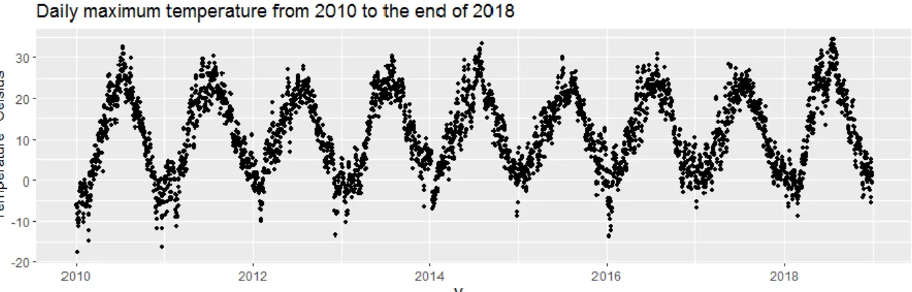
To get a larger picture of the data to be forecasted Figure 3.1 below is included, where we can see the observed maximum temperatures in Uppsala from 2010 until the end of 2018, corresponding to 3287 observed values. In the upper figure, we can see that there is a frequent recurrent pattern or seasonality in the data with low temperatures in the beginning and the end of the year and high temperatures in the summer.
Figure 3.1. Overviewing represented data of daily maximum temperatures in Uppsala from 2010 until the end of 2019.
13
Further, it seems to be a constant mean throughout the years of the time series. In the lower figure, we can see the variability in temperature for every month within the given period. The middle line in the boxes is the median value and the lower and upper bounds of the boxes are the first and third quartiles.
The dataset used for this study contains daily observations and is narrowed down to contain data from 1 January 2017 to 31 March 2019. The oldest observations are omitted for the training of the models to not be too time-consuming. The omitting of the oldest observations should not affect the results very much since the used methods are simple and the patterns in the data are recurring. The dataset has no missing values and is corresponding to 820 observations of the maximum temperature in degrees Celsius registered daily. The first 730 observations serve as the training set and the last 90 observations serve as the test set. The data are collected two times a day with a 12-hour interval from 18 UTC the day before until 18 UTC the representative day, where the highest temperature of the day is registered in the dataset (SMHI, 2019).
The statistical software and programming language R is used for this thesis. The mainly used package for this thesis is the complete time series package forecast written by Hyndman et al. (2020). The package includes tools for working with and graphically displaying time series data as well as methods for analyzing the time series and estimating forecasting models. Several large imports are included in the package e.g. the ggplot2, zoo, and nnet packages (Hyndman et al., 2020).
14
4. Results
Table 4.1. Properties of ARIMA when estimated using the training set.
ARIMA
(𝑝, 𝑑, 𝑞) (4, 1, 4)
𝐴𝐼𝐶𝑐 3506
P-VALUE (LJUNG-BOX TEST) 0.8877
The ARIMA model is estimated on the training dataset consisting of 720 observations from 1 January 2017 to 31 December 2018. The model is fitted by the auto.arima function where different properties of the order of the model are automatically compared by looking at the AICc of the model, without any approximations. The residuals of the fitted model are investigated both visually and by doing a Ljung-Box test to make sure that no autocorrelation is left in the residuals i.e. the residuals are close to white noise. The residual diagnostic of the chosen model is presented in Appendix A. In the table above, the properties of the best ARIMA are presented. The NNAR model is fitted to the training dataset by the nnetar function where the number of lags denoted 𝑝 is decided automatically by minimizing the AIC just like a regular AR model. The number of nodes in the hidden layer is decided by 𝑘 = (𝑝 + 1)/2. The automatically decided number of lags from the nnetar function is compared with choosing the number of lags of an AR model through the auto.arima function, with MA and the first difference being set equal to zero to alter the hyperparameters and avoid overfitting.
Table 4.2. Properties of NNAR when estimated using the training set. The presented AICc is the AICc from the AR process when choosing the order to include in the input layer.
NNAR
(𝑝, 𝑘) (5, 3)
𝐴𝐼𝐶𝑐 (ORDER OF AR) 3538
15
Due to the risk of overfitting with neural networks, the model with the least lags which still has residuals indistinguishable to white noise i.e. a non-significant Ljung-Box test is chosen as the best model, see Appendix B for residual diagnostics. The residuals of the final model are investigated just like in the case of fitting the ARIMA and the properties of the model are presented in the table above. Since the starting weights of the NNAR are determined randomly the function set.seed is used and set to
set.seed(12345) to be able to reproduce the estimations of the weights in the NNAR.
The naïve method has no hyperparameters to be estimated since it only uses the last observed value for predictions and is not needed to be fitted to the training set. The residuals of the naïve method from the training set are, however, still included in Appendix C.
4.1 One-step Forecasting
The one-step forecasts are done through a walk forward validation on the test set consisting of 90 observations from the 1 January 2019 to the 31 of March 2019. For each model, every forecast is compared with the real value in the test set and an absolute error (AE) is calculated and then summed up and averaged, resulting in the MAE. In Table 4.3 below we can see the forecast accuracy presented in MAE and MASE for one-step forecasts for the three models ARIMA(4, 1, 4), NNAR(5, 3), and naïve. The MAE is calculated and presented on the scale degrees Celsius, which means that the MAE represents how many degrees Celsius the different models on average are wrong with compared to the observed values, in absolute values. The MASE is scale-independent and calculated by taking the MAE of the models divided by the MAE of the naïve method from the training set i.e. the in-sample dataset.
Table 4.3. The forecast accuracy of ARIMA, NNAR, and naïve for one-step forecasts, with MAE in degrees Celsius and MASE being scale independent.
MODEL MAE MASE
ARIMA 2.245 1.048
NNAR 2.227 1.039
16
The lowest forecast error i.e. the best forecast accuracy is bolded in the table and we can see that NNAR has slightly better forecast accuracy than the other methods, with a MAE at 2.227 and a MASE at 1.039. This means that forecasts by the NNAR model on average are wrong with 2.227 degrees Celsius. By looking at the MASE value at 1.039 we can see that the MAE of the forecasts produced by the NNAR is slightly worse than the MAE of the in-sample naïve since it is larger than 1. The second-best one-step forecasts are produced by the ARIMA with a MAE of 2.245 degrees Celsius and a MASE at 1.048. The worst one-step forecasts are produced by the naïve method with a MAE of 2.301 degrees Celsius and a MASE at 1.074. It should be noted that the MAE of the forecasts using the naïve method on the test set is larger than the MAE on the training set i.e. the test set has larger differences between observations and could be harder to predict.
In the figure below the variation in one-step forecast errors for the three models ARIMA, naïve, and NNAR is presented. The result of the highest accuracy is not very apparent in the figure since the differences in variation are small between the errors of the models.
Figure 4.1. Distributions of one-step forecast errors for the ARIMA, naïve, and NNAR regarding the one-step forecasts on the test data.
17
The NNAR has the highest median error even though the model has the lowest MAE, which could be because the model seems to have the smallest errors above the third quartile. The figure indicates that the NNAR could have a smaller variation in errors compared to the two other models. The errors of the naïve method are most obvious to differ from the two other models even though the first quartile and the median are very similar to the other two models. What is obvious, however, is that the third quartile and the maximum value of the naïve are higher than the once of the NNAR and the ARIMA.
4.2 Multi-step Forecasting
The multi-step forecasts follow the same procedure as for the one-step forecasts and are tested on the 90 observations of 2019. However, the obtained forecasts for evaluation are only 86 since the forecast horizon is ℎ = 5, making predictions for two to five steps in the future, resulting in 90 − (ℎ − 1) observations.
In the table below we can see the multi-step forecasts for the ARIMA, NNAR, and naïve i.e. for forecast horizons two, three, and five days into the future. The ARIMA and NNAR model makes stepwise predictions for every day into the future and uses the predicted values to predict the succeeding days iteratively. The naïve method, however, always predicts its forecasts to be equal to the last observed value. This means that the forecasts for two, three, and five days into the future always are the same when having the same last observed value.
Table 4.4. The forecast accuracy of ARIMA, NNAR, and naïve for more than one step forecasts, with MAE in degrees Celsius and MASE being scale independent.
H = 2 H = 3 H = 5
MODEL MAE MASE MAE MASE MAE MASE
ARIMA 2.821 1.317 2.932 1.368 3.397 1.585 NNAR 2.764 1.290 2.892 1.350 3.346 1.562 NAÏVE 2.897 1.352 3.057 1.427 3.437 1.604
18
In Table 4.4, we can see that the NNAR has the best predictions for all forecast horizons with a mean absolute error of 2.764 degrees Celsius for two-step forecasts. Together with a mean absolute error of 2.892 and 3.346 degrees Celsius for three and five-step forecasts respectively. The second-best forecast accuracy is obtained by the ARIMA and the worst by the naïve method for all forecast horizons. Further, we can see that all methods have larger absolute errors for longer forecast horizons and that the MASE of all methods is increasing correspondingly. The mean absolute scaled errors are gradually increasing for all methods with longer forecast horizons since the scaling component always is the MAE of the one-step forecasts from the in-sample naïve.
In Table 4.5 below, we can see the results of the DM-test assessing whether a significant difference among the forecasts from the different methods is apparent. With the null hypothesis that there is no difference and a one-sided alternative hypothesis. To be noted is that the DM-test is used in this thesis to assess for the potential difference in forecasts in an out-of-sample period and is not necessarily an indicator of which underlying model is the best one. The significance level in this thesis is set to be the standard 0.05 and the significant p-values in the table below have been bolded.
Table 4.5. One-sided Diebold-Mariano test for predictive accuracy, comparing the forecast accuracy of forecasting methods.
DIEBOLD-MARIANO TEST
H = 1 H = 2 H = 3 H = 5
ACCURACY p-value p-value p-value p-value
NNAR > ARIMA 0.091 0.298 0.522 0.614 NNAR > NAÏVE 0.039 0.048 0.174 0.367 ARIMA > NAÏVE 0.105 0.109 0.206 0.326
19
From the DM-tests, we can on a five percent significance level reject that the NNAR and the naïve forecasts are equally accurate on one-step and two-step forecasts in favor of the alternative that the NNAR has more accurate forecasts. Even though the NNAR has lower MAE than the ARIMA and the ARIMA has lower MAE than the naïve for all forecast horizons, the differences are not large enough to be able to reject the null hypothesis.
20
5. Discussion
What can be seen in the result is that we have a hierarchy among the different forecasting models in terms of forecasting accuracy for the used test set. The best i.e. most accurate method for the used dataset is the NNAR, the second-best is the ARIMA and the method with the lowest accuracy is the naïve method, which is consistent for all forecasting horizons. The differences in MAE for the methods are, however, not consistently getting larger when conducting forecasts with larger forecast horizons. The NNAR for example, which had the best accuracy for every forecast horizon had a decrease in difference in MAE compared to the other two models when going from three steps to five steps into the future. This could be an indication of the NNAR not having an increasing difference in accuracy compared to the other two methods for larger forecast horizons but have higher accuracy for at least the five-step horizon due to lower errors in the shorter forecast horizons.
The differences in MAE between the different methods are not very large which raises the question of whether the differences are large enough to say that one model is more accurate than the others. By testing with the formal Diebold-Mariano test for comparing forecasts, the methods with significantly better forecasting accuracy compared to the other methods could be determined. The only same-step forecasts where the null hypothesis of two forecasts being equally accurate could be rejected is when comparing the NNAR and naïve for one and two-step forecasts. Therefore, we can assert that the NNAR is better at forecasting the daily maximum temperature than the naïve for the used dataset and the mentioned forecast horizons. For the comparison of NNAR and ARIMA together with ARIMA and naïve, we can say that NNAR and ARIMA have a higher forecasting accuracy in the used dataset but not that they are significantly better.
Diebold (2015) gives his own take on comparing forecasts and models in his article
Comparing Predictive Accuracy, Twenty Years Later: A Personal Perspective on the Use and Abuse of Diebold-Mariano Test*. His opinion is that the DM-test should not
be used to make general conclusions when comparing models but rather to compare specific forecasts. Together with the fact that the forecasts are done on only one test set and only three months out of twelve, it is no point in making assertive
21
generalizations about which model is the best for all periods of a year or all years in general. Even though we could in Section 3, see that the time series had a very recurrent pattern we can still see slight variability in the time series which could affect the conclusions when only testing on three months which makes the generalizability low. This argument could be strengthened by the fact that the MASE always is larger than one for all methods and forecast horizons. Even though the naïve method is distinctly worse in forecasting the test period, the in-sample naïve had a lower MAE than both the ARIMA and NNAR for the test set. This could be an indication that there is some variability in the data depending on the different seasons of a year which could affect the results of the performance of the different methods. We do, however, have a strong indication that the NNAR could be a better forecasting method, at least compared to the naïve since the difference for some forecast horizons is significant in favor of the NNAR. Especially since the data follows a closely similar pattern through every year and can be assumed to have the same recurrent pattern in the future. This would imply that the use of an NNAR would be a better method compared to only estimate the maximum temperature of a day solely on the maximum temperature of yesterday.
One of the reasons why the test is not made iteratively over many test periods in this thesis is due to the computational heaviness of primarily the neural network. Hyndman (2019) stated when summarizing the evolution of forecasting competitions that there is a consensus in the field of forecasting, that complex methods such as neural networks are performing badly for univariate time series. Partially because many data points are needed. A large dataset is prioritized at the expense of generalizability in this study for the neural network to have enough data points to learn from. This gives the neural network the needed circumstances for good forecasts and could shed new light on the usefulness compared to the results of previous forecast competitions when the datasets been small. There are a lot of data points for maximum temperatures for a lot of different areas in Sweden, which makes the field a potentially good one for the use of a neural network.
An interesting aspect of the result from the conducted study is that the NNAR performs better than for example the ARIMA, which could be due to the use of a large sample size in the training dataset. Many of the comparisons with conclusions
22
of neural networks being bad methods for forecasting in previous studies, compared to older statistical methods has been made with small datasets even though neural networks are known for requiring many observations. In a thesis by Naz (2015) comparing the temperature in Umeå, the author concluded that the ARIMA was the best model compared to other classical forecasting methods which were both univariate and multivariate. Further, the author found that the ARIMA in many cases performed better than the forecasts made by SMHI. The result that the NNAR even could outperform an ARIMA for the Uppsala dataset used in this study makes it interesting to do further comparisons. To investigate how good an NNAR and ARIMA could perform when comparing them for a variety of datasets and periods, of observed maximum temperatures in Sweden, to be able to make more generalizable conclusions.
In conclusion, the NNAR model had the best forecast accuracy for all forecast horizons when predicting the maximum temperature in Uppsala, which suggests that the method could be superior to the other for this purpose. To more emphatically state this conclusion and to be able to interpret this result as generalizable a larger research is encouraged.
23
Bibliography
Brownlee, J., 2019. How to Backtest Machine Learning Models for Time Series
Forecasting.
https://machinelearningmastery.com/backtest-machine-learning-models-time-series-forecasting/, (Accessed 2020-03-15).
Cryer, J.D., and Chan, K., (2008). Time series analysis: with applications in R. Springer, New York, 2nd edition.
da Silva I.N., Hernane Spatti D., Andrade Flauzino R., Liboni L.H.B., dos Reis Alves S.F., (2017). Artificial Neural Networks. Springer, Cham.
Diebold, F.X. and Mariano, R.S., (1995). Comparing predictive accuracy. Journal of
Business and Economic Statistics, 13(3), 253-263.
Diebold, F.X., (2015). Comparing Predictive Accuracy, Twenty Years Later: A Personal Perspective on the Use and Abuse of Diebold–Mariano Tests. Journal of
Business & Economic Statistics, 33(1), 1-22.
Feedforward Deep Learning Models. (n.d.). In GitHub. Accessed May 2, 2020, from http://uc-r.github.io/feedforward_DNN
Hyndman, R.J., and Athanasopoulos, G., (2018). Forecasting: principles and
practice, OTexts, Melbourne, 2nd edition. https://otexts.com/fpp2/, (Accessed on
2020-02-22).
Hyndman, R.J., (2019). A brief history of forecasting competitions. International
Journey of Forecasting, 36(1): 7-14.
Hyndman, R.J., Athanasopoulos, G., Bergmeir, C., Caceres, G., Chhay, L., O'Hara-Wild, M., Petropoulos, F., Razbash, S., Wang, E. and Yasmeen, F., 2020. forecast:
Forecasting functions for time series and linear models. R package version 8.10.
24
Makridakis, S., Spiliotis, E., and Assimakopoulos, V., (2019). The M4 Competition: 100,000 time series and 61 forecasting methods. International Journal of
Forecasting, 36(1): 54-74.
Naz, S., 2015. Forecasting Daily Maximum Temperature of Umeå. Master diss.,
Umeå University. urn:nbn:se:umu:diva-112404
SMHI, 2019. Vad gör SMHI?. https://www.smhi.se/omsmhi/om-smhi/vad-gor-smhi-1.8125, (Accessed on 2020-02-20).
Taylor, J.W. & Buizza, R., 2003. Using weather ensemble predictions in electricity demand forecasting. International Journal of Forecasting, 19(1): 57-70.
Weather forecasting. (n.d.). In Wikipedia. Accessed May 11, 2020, from https://en.wikipedia.org/wiki/Weather_forecasting#cite_note-87
25
Appendices
26
27
Appendix C