Monitoring of Micro-sleep and Sleepiness for the Drivers Using EEG Signal

School of Innovation, Design and Engineering

Monitoring of Micro-sleep and

Sleepiness for the Drivers Using EEG

Signal

Thesis basic level, Computer

Science

15 Credits

Shahina Begum (shahina.begum@mdh.se)

Examiner:

Peter Funk (peter.funk@mdh.se)

School of Innovation, Design and Engineering (IDT) Mälardalen University

ABSTRACT

Nowadays sleepiness at the wheel is a problem that affects to the society at large rather more than it at first seemed. The purpose of this thesis is to detect sleepiness and micro-sleeps, which are the source that subsequently leads to drowsiness, through the study and analysis of EEG signals. Initially, raw data have some artifacts and noises which must be eliminated through a band pass filter. In this thesis EEG signals from different persons are analyzed and the feature extraction is carried out through the method Fast Fourier Transform (FFT). After that, the signals are classified to get the best result. To do this, the method Support Vector Machine (SVM) is used where the feature vectors, which have been extracted previously, are the input. The data are trained and tested to get a result with an accuracy of 77% or higher. It shows that EEG data could be used helping experts in the development of an intelligent system to classify different sleeping conditions i.e., micro-sleep and micro-sleepiness.

ACKNOWLEDGEMENT

This thesis would not be possible without the help of some persons. We are very grateful to our supervisor Shahina Begum for her suggestions, helps, and guidelines and especially for her valuable time in different stages of this thesis. We would like to thanks also to Shaibal Barua for his high helps, suggestions and especially for his valuable spent time to explain us the hardest parts of this thesis.

Finally, we are grateful to our friends and our families for their supports and affection that they try to send us from Spain.

Västerås, May 2013

CONTENTS

SUPPORT VECTOR MACHINE ... 31

RELATED WORK ... 41

Extraction of Feature Information in EEG Signal ... 41

Sleepiness and health problems in drivers who work driving some kind of vehicle with nocturnal and shift works ... 43

SVM Regression Training with SMO ... 48

EVALUATION AND CONCLUSION ... 52

FUTURE WORK ... 55

LIST OF FIGURES

Figure 1: representation of the sleep macrostructure (states I, II, III and IV and REM)... 17

Figure 2: an example of cyclic alternating pattern (CAP) in sleep stage 2 [12-13]. ... 18

Figure 3: phase A subtype A1 ... 19

Figure 4: phase A subtype A2 ... 19

Figure 5: phase A subtype A3 ... 19

Figure 6 ... 22

Figure 7 ... 22

Figure 8 ... 23

Figure 9: filtered signal ... 23

Figure 10: original signal ... 23

Figure 11 ... 28

Figure 12: frequency response of the filtered signal ... 29

Figure 13: cost1(z) ... 32

Figure 14: cost0(z) ... 32

Figure 15 ... 33

Figure 16 ... 34

Figure 17: polynomial kernel ... 35

Figure 18: perceptron ... 35

Figure 19: Gaussian radial basis function ... 36

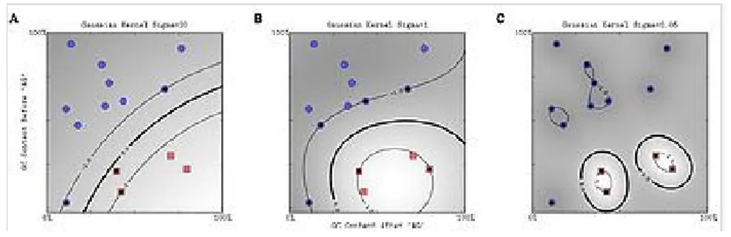
Figure 20: Support vector Machine for Regression - Radial Basis Kernel ... 37

Figure 21: insomnia ... 45

Figure 22: sleepiness ... 46

Figure 23: cases with psychological symptoms ... 46

Figure 24: cases with musculoskeletal symptoms ... 47

Figure 25: cases with gastrointestinal symptoms ... 47

Figure 26: accuracies of SVM... 53

LIST OF TABLES

Table 1: Advantages and disadvantages of classifiers………12 Table 2: EEG waveforms representation………15

LIST OF ABBREVIATIONS

BRIR Band Relative Intensity Ratio. CAP Cyclic Alternating Pattern. CBR Case-Based Reasoning DFT Discrete Fourier Transform. DWT Double Wavelet Transform. EEG Electroencephalography.

FT Fourier Transform.

FFT Fast Fourier Transform. FIR Finite Impulse Response.

GT Gabor Transform.

ICA Independent Component Analysis. IIR Infinite Impulse Response.

LDA Linear Discriminant Analysis.

NN Neural Networks.

NREM Non Rapid Eye Movement.

OSH Optimal Separating Hyper plane. PSD Power Spectrum Density.

QP Quadratic Programming.

RBF Radial Basis Function. REM Rapid Eye Movement.

INTRODUCTION

Electroencephalography (EEG) is a neurophysiological examination based on the registration of brain bioelectrical activity at baseline sleep, waking or sleeping, at mental stress and during various activations by a set of electroencephalography's instruments. With EEG signals the behavior of the brain can be studied on many different situations and even brain diseases, or something like that, can be detected. This thesis focuses in the analysis and study of these EEG signals to detect drowsiness in drivers in order to the experts can develop an intelligent system which helps to classify different sleeping conditions and try to provide a possible solution to this problem which is the causative of some accidents on road.

Objective

The objective of this thesis is to detect micro-sleeps, which are the source that subsequently leads to sleepiness in drivers, through the analysis and study of EEG signals. When these pathologies are detected, it is necessary to obtain an accuracy of 77% or higher from data in order to the experts can develop an intelligent system which helps to classify different sleeping conditions. Support Vector Machine (SVM) [9] algorithm has been applied to obtain the best accuracy from data. In addition, Fast Fourier Transform (FFT) is the method that has been chosen to extract features from EEG signals. These features have been classified to assess the system along with features obtained from filtered signals. A study of these methods and their results is shown in this thesis.

Problem domain

Sleepiness at the wheel is a problem that affects society at large rather more than it at first seemed and it is an important causative of accidents on road. It is a state which drivers are almost asleep. In addition, other common state of this kind of pathologies is the fatigue, which is an extreme tiredness that results from mental or physical activity. It refers to an inability to keep awake. Sleepiness is also called grade of vigilance which is a state where one is prepared for something to happen [2]. Besides, the main factors of sleepiness are the time spent to carry out a task, the motivation to make that task, monotony of the task, temperature, sound, amount of light, oxygen content, and the amount of sleep during night.

Methodology

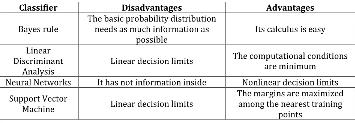
In this thesis, the classification method that has been chosen is SVM. Comparing with other methods, the table 1 shows the reason for SVM has been chosen against other methods. This method is simpler than others and it has a quite low empirical error. Before that, it is necessary to analyze all of the data, to do this, the signals are filtered, then all of the frequencies must be calculated using the method FFT (Fast Fourier Transform) and, finally, all features have to be extracted to use them in the algorithm SVM. In order to classify different data, it is necessary to choose the SVM and the kernel type. For the first one multiclass is chosen and for the second one RBF is chosen because it returns the optimal result. Besides, the appropriate parameters are selected based on trial and error.

Table 1: Advantages and disadvantages of classifiers

Classifier Disadvantages Advantages

Bayes rule The basic probability distribution needs as much information as

possible Its calculus is easy

Linear Discriminant

Analysis Linear decision limits

The computational conditions are minimum

Neural Networks It has not information inside Nonlinear decision limits Support Vector

Machine Linear decision limits

The margins are maximized among the nearest training

points

Organization of thesis

The rest of this thesis is arranged as follows:

• _{Background. It explains the problem domain which is basis of this thesis.} • _{Methods. It describes different methods that are used in this thesis.}

− _{Implementation. It explains all of the methods and explains how each of them} has been implemented in this thesis.

• _{Related work. It explains works that are related to the thesis work described in the} report.

BACKGROUND

The background of the area of micro-sleeps and drowsiness, where the basis of this thesis is focused, is explained below.

Sleepiness in drivers

Micro-sleeps are the main factor of sleepiness in drivers and cause one in four fatal accidents on highways [1]. Micro-sleeps are very short periods of sleep because of extreme tiredness. Those affected are mostly male and middle-aged, overweight, increased frequency of snoring, morning tiredness and hypertension [1]. These sleepy drivers are 11 times more likely to have an accident [1]. A percentage of 54% suffer from sleep-disordered breathing [1]. Drowsy drivers with respiratory diseases during sleep are six times more likely to have an accident [1]. Keep in mind that sleep respiratory diseases are an independent factor that explains most accidents usually of sleepy drivers. The hours of the day with increased risk of drowsiness are between 13:00 and 16:00 hours [1].

Some tips are suggested to avoid sleep at the wheel, like for example listen to the radio, eat candy, chew on gum or open the window to let in fresh air. However, these remedies have minimal effectiveness. "Drowsiness is persistent and eventually sooner or later will beat us," says the study [1]. The only effective remedy is to stop the vehicle in a safe place and sleep for about twenty minutes. If drowsiness is light, a small walk will reactivate the blood circulation and muscle exercise.

On the other hand, there are a lot of studies done on this area, and all of them show the same result. All of the people that work driving vehicles (it does not matter the kind of vehicle) above all at night, show problems that may affect the health. This is caused for subjecting the body to sleep at times that are not the most appropriate. In fact, these workers are more likely to have depression, insomnia and sudden mood swings. Almost all of them are forced by their jobs to sleep during the day; therefore they can be exposed to be awakened by external factors in the normal daily life. This, combined with the teaching hours, produces an alteration in the normal rhythm of sleep causing bad consequences on the health of workers.

Besides, at first glance it seems that does not cause much impact on the health of workers, but with the passage of time, when an employee has been 25 years or more in this kind of job, the negative consequences of this lifestyle are palpable and noticeable.

Other important risk of the sleepiness in the drivers is the high chance of cause accidents. At night, one of the main causes of accidents is the sleepiness in the drivers because this state is which the workers are almost asleep. It refers to an inability to keep awake. In addition, other common state from this kind of workers is the fatigue, which is an extreme tiredness that results from physical or mental activity. The sleepiness is sometimes also called grade of vigilance. This grade of vigilance is a state where one is prepared for something to happen [2].

In addition, the main factors of sleepiness are the amount of sleep during the night and the time spent to carry out a task. Of course, other factors of sleepiness are the monotony of the task, the motivation to make that task, sound, temperature, oxygen content and amount of light.

So, for these reasons it is considered very important to make a study of monitoring of micro-sleep and sleepiness for the drivers using EEG signal. To do this, some steps are followed as it is shown below.

DATA ANALYSIS

Data analysis is comprised of some fundamental steps like pre-processing, feature

extraction and classification of EEG signals.

Pre-Processing

EEG signals are very sensitive to external factors that are independent from the brain, like for example broken EEG electrodes, blinking and movement of eyes, dried electrodes, stretching of muscles, excessive electrodes gel, etc. These external factors are called artifacts and they can be removed applying the appropriate filter. A wide range of artifact removal methods exists, including:

• Subtraction method. Supposing that contaminated EEG signal is a linear combination of noisy signal and original EEG signal, noise from contaminated signal is subtracted to recover the original signal [3].

• Min-max threshold. It sets maximum or minimum allowed amplitude for a concrete time length [4].

• Gradient criterion. It sets, relative to intersample time, an artifact threshold based on point-to-point changes in voltage [4].

• Simple amplitude threshold. It sets positive and negative amplitude thresholds and considers the data out of this range are an artifact [4].

• Independent component analysis (ICA). Source separation is performed to split components that have statistical difference and, after multiplying by an unknown matrix, with as little assumption about the source signal or this matrix as possible, it recovers N linearly mixed source signals [4].

So, pre-processing is the step where the noise is removed from the original signal. Feature extraction

This is the step after pre-processing of EEG signals. It proceeds to calculate frequency amplitudes from filtered signals. There are several ways to calculate it, using Short Time Fourier transform (STFT), Fast Fourier transform (FFT) or Wavelet Transform (WT). The disadvantage of Short Time Fourier Transform against Wavelet Transform is the finite length window that in spite of increase the time, resolution reduces the frequency resolution [5]. The main goal of this step consists in divide the signal in different frequency ranges (alpha, beta, theta, delta…). These ranges allow studying the signals’ behavior.

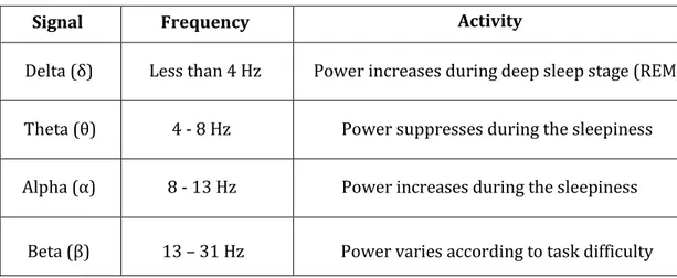
The next table shows different features with their frequency ranges and a brief description of their activities.

Table 2: EEG waveforms representation

Signal Frequency Activity

Delta (δ) Less than 4 Hz Power increases during deep sleep stage (REM) Theta (θ) 4 - 8 Hz Power suppresses during the sleepiness Alpha (α) 8 - 13 Hz Power increases during the sleepiness

• Alpha waves are more active in occipital regions of the brain [4] and with closed eyes. These waves are dominant when the brain is doing no activity, in micro-sleeps or sleepiness conditions. In stressful situations, the power of alpha waves falls down.

• Beta waves are more active in central and frontal regions of the brain. Beta waves are dominant in tension states and their power varies according to task difficulty [7].

• In theta waves the power increases under stress or mental tasks [6]. • In Delta waves the power increases during deep sleep stages (REM) [7]. Classification

This is the step after feature extraction of EEG signals. There are some interesting algorithms to proceed with the classification.

• _{Support Vector Machine (SVM). Given a points set, subset of a larger set (space),} in which each of them belong to one of two possible categories, SVM algorithm builds a model that predicts whether a new point (whose category is unknown) belongs to one category or the other [9].

• _{Neural Networks (NN). Independent processing units are assembled and}

connected with each other. Moreover, these generate a function of their total inputs [10].

• _{Linear Discriminant Analysis (LDA). The data are divided into hyper planes to}

represent different classes. Due to linear nature of EEG data, is not recommended to use LDA [8].

• _{Bayes Rule. Posterior probability of a feature vector is computed to belong to a} particular class. In addition, feature vector is located into a class where it belongs to the highest probability [11].

METHODS

In recent years the sleep study has increased because it is essential for both physical and mental restoration. The brain is active during sleep and the brain waves are changing shape and speed as the night progresses.

Sleep-wake disorders that adversely affect the health and the life quality of people can be predicted with the help of these waves. These disorders include problems falling asleep or keep it stable, to be wide awake during the day, to keep schedules sleep / wake reasonable, among other things, disorders prognosis based on the study of the activity electrical brain (called EEG) during sleep. This activity is recorded in different areas of the scalp and the signals are stored for later analysis.

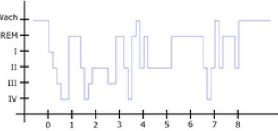
The polysomnography is a sleep study by recording of electrical brain waves (EEG), electrical activity of muscles and eye movements. From this study comes sleep macrostructure consisting classification of sleep recording in 4 states NREM (Non Rapid Eye Movement) and REM state (Rapid Eye Movement). This classification is done by reviewing time segments (called epochs) from the polysomnography, which analyzes the signal characteristics such as frequency content and some typical patterns to assign an unique state.

The following graph shows the hypnogram, which is a temporary representation of the different states of sleep for 8 hours recording. This graph allows an overview from the distribution of wakefulness and the different sleep stages.

Then it is necessary to study the microstructure sleep. From this study it is defined Sleep Cyclic Alternating Pattern (CAP) which is composed of two phases, phase A, comprising a variation of EEG activity abruptly both in frequency and in amplitude (at least one third higher compared activity to the base) and phase B which is the rank of base brain activity between two phases A. Both phase A and B must have duration of 2-60 seconds. The sum of a phase A and B is equal to one cycle.

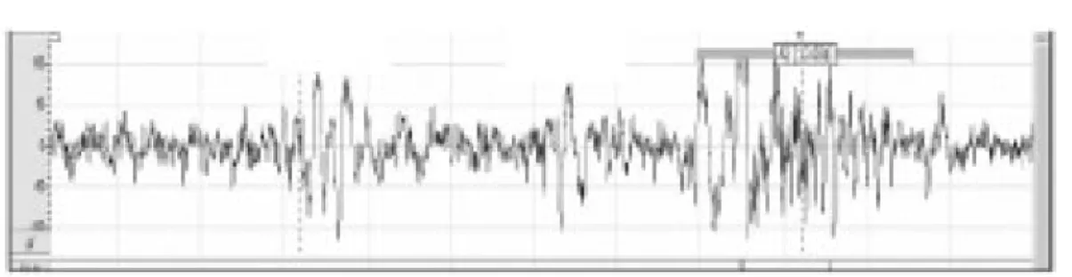
Figure 2: an example of cyclic alternating pattern (CAP) in sleep stage 2 [12-13].

The activities in phase A can be classified into three subtypes. Subtype classification is based on the proportion of high voltage slow waves (EEG synchronization) and rapid rhythms of low amplitude (asynchrony) throughout the phase A duration. Three subtypes in phase A are described as follows:

• Subtype A1: The EEG synchrony is the predominant activity. It must contain less than 20% of EEG desynchronization in the phase A entire duration.

• Subtype A2: EEG activity is a mixture of fast and slow rhythms with 20-50% of phase A by EEG desynchronization.

• Subtype A3: The EEG activity rhythms are based on low voltage fast EEG desynchronization over 50% of phase A.

These are some examples about different subtypes A.

Figure 3: phase A subtype A1

Figure 4: phase A subtype A2

It is interesting and important to explain the CAP and its functioning because all of the data-sets that have been chosen for this thesis are from CAP Sleep Database from Physionet [12-13].

With data-sets obtained, it proceeds with analysis techniques to study how micro-sleeps influence in the drivers.

PRE-PROCESSING

The signals have been taken with 1 minute duration. These signals belong to S0, S1 and S2. These are the different sleep stages. Stage 0 (S0) refers to be awake, stage 1 (S1) is a sleepiness state that lasts few minutes because it is the transition between wakefulness and sleep and hallucinations can occur in both the input and the output of this phase (5% of total sleep time) and stage 2 is a light sleep state, it is to say, lower both heart rate and respiratory, suffering variations in traffic brain, lulls and sudden activity, which makes it harder to wake up and there is a process in which beats are extremely low in some cases because the sleep is so deep that brain no longer registers contact with the body and sends a pulse to corroborate life (50% of the time).

As already mentioned, raw EEG signals are of extremely small magnitude, so that they are easily contaminated by noise and interferences. It is for this reason, the first link in the chain of processing involves a set of steps intended to clean raw EEG signals and remove any interference component. This stage consists of several phases. First, raw EEG signals are filtered using a digital band pass filter on each channel.

These filters have the advantage of removing any interference of 50 Hz from the mains. Furthermore, the use of band pass filters allows EEG signal downsample from its original sampling frequency 512 samples per second to a more manageable 128 samples per second per channel. This is done without loss of information and helps to make the system faster.

Then, an algorithm is applied, to remove from the raw signal unwanted artifacts that result from the user’s muscle activity. The eye movement, blinking, swallowing, and limb movements generate strong EEG components that mask the components generated by neurons and those interested in our analysis.

There are several techniques to reduce the effect of these artifacts. First, for the artifacts generated by eye movements and blinking, additional sensors may be located close to the eyes which collect the called electromyogram (i.e., the electrical signals generated by muscle activity). These signals may be used as the reference input to a special type of filter called adaptive noise canceller, and rearranging filters artifacts generated by the eyes, to be equal to the interference that contaminates raw EEG signals. This is carried out using a feedback algorithm that uses correlation analysis to learn the interference’s characteristics on each EEG channel. Once the system has learned these features, the output of the adaptive filter may be subtracted from the raw EEG signal, thereby producing a "clean" version without artifacts generated by the eyes.

Secondly, it applies an algorithm that compares fast and slow currents of differences between various EEG electrodes, in order to eliminate other artifacts resulting from body movements.

Third, it is a fact that many noise components, especially those outside from the human body (e.g. machinery, traffic, vibrations etc.), are in signals that are common to all of the EEG channels. But this study is interested in local variations between EEG signals. Therefore an effective way of eliminating this global interference is to use a spatial Laplacian filter which has the effect of emphasizing the differences between individual channels above larger global effects. Laplacian spatial filter is a relatively simple operation which consists in, subtracting the signal from each electrode EEG signals, the average of their nearest neighbors.

Finally, it is not uncommon for one or more sensors produce an erroneous output, usually due to poor contact with the user’s scalp (although electrode gel is used in order to minimize this failure). A limitation algorithm is used in order to mitigate this problem (thresholding), which eliminates those channels that produce incorrect signals to avoid that these suffer a subsequent analysis and processing.

Note that usually on these cases of study a lot of channels are used, as for example in raw data taken from CAP Sleep Database in Physionet [12-13]. As a side note, it is mentioned that more sensors also imply more time signal processing.

IMPLEMENTATION

In this chapter, it is explained how to proceed with the signal pre-processing. To do this, it is used Matlab, a software with good interactive environment which is used, among other things, to signal processing.

It has not enough material to perform all of the filtering tasks described above, but at least Matlab is used in order to carry out the implementation of a band pass filter which will allow to remove noises and artifacts from the original signal extracted from the patient. As a consequence of the implementation of this filter, it will be possible to continue with the previously filtered signal processing.

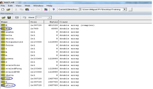
First of all, it is proceeded to open Matlab and load the original signal. Then, it is designed the band pass filter, to do this, it is necessary to go to Start/Toolboxes/Filter

Design/Filter Design & Analysis Tool. The next figure shows the process:

Figure 6

Once there, it is selected a band pass filter, IIR method and limits have to be established to pass a certain frequency rank, which in this case will be between 3 Hz and 100 Hz. Frequency values within these limits are really interesting to carry out this thesis, and the frequency components values near the frequency that it allows to pass will be 4 Hz and 99 Hz respectively.

A band pass filter is a type of electronic filter that allows passing a certain frequency rank from a signal and attenuates the pass of the rest. In design method, it has chosen IIR because it is able to fulfill the same requirements than FIR but with less filter order. This is important when implementing the filter, therefore it has lower computational burden. Then the filter is exported to the workspace where a new variable called Num is created, which will refer to the just designed filter.

In the next step the filter is applied to the signal, to do this, it is used the instruction

yfilt = filter(Num,1,val) where yfilt is the filtered signal name and filter is the function with

which the filter is applied. This function has three parameters, Num, 1 and val; Num refers to the just designed filter, 1 is a constant and val is the original signal.

Figure 8

When the signal has been filtered, the result is as follows:

Here, the big difference with the original signal can be appreciated with all of the artifacts and noises removed.

FEATURE EXTRACTION

This is possibly the most critical step in the signal processing. The goal of this step is to create a manageable and meaningful representation of the original EEG signal (although clean), in order to maximize the potential success of qualifiers and in turn the overall system performance. A second objective of the feature extraction phase is to compress data without loss of relevant information in order to reduce the number of input variables in qualifiers (in order to operate in real time). There are several approaches that may be adopted in the feature extraction phase and actually find just the right to do so is an active target of this thesis.

A simple method of feature extraction is what is called the method "band spectral power" which each channel is applied to a bank of four digital band pass filters. These filters have pass bands centered on four frequency bands in conventional EEG signal analysis: delta waves (0-4 Hz), theta (4-8 Hz), alpha (8-13 Hz) and beta (> 13 Hz). These frequency bands have been studied for decades and are known to represent interesting forms of brain activity. For example, a strong alpha component means that the subject is very relaxed. At the output of these band pass filters the instantaneous power is measured using a moving average filter sliding window. On this way each channel EEG raw signal is transformed into a set of four power measurements that are updated regularly.

A second feature extraction method is called autoregressive modeling. Through this approach, it is attempted to predict the signal’s nth sample from a linear combination of a number of previous samples. The best linear predictor coefficients are the features which constitute the entrance to the qualifying. This is exactly the same technique that is used in order to compress and transmit voice signals over digital telephone lines (fixed and mobile). It is also extending the technique to treat appearance multichannel EEG data, although this is proving quite problematic because of the intensive calculations required to find a model of real-time multi-channel signal. Studies in this area continue.

This thesis focuses on getting the four classical frequency bands in EEG signal analysis: delta waves, theta, alpha and beta, but in this case it focuses especially on the alpha, beta and theta waves because what really it is wanted to analyze are micro-sleeps and how they affect in the drivers, therefore, sleep stages to be discussed in this thesis are S0, S1 and S2, which have been explained above. Delta waves have been discarded because they are part of phases of deep sleep (S3 and S4), which are not part of the analysis. To do

Fast Fourier Transform

Discrete Fourier Transform transforms a mathematical function into another, obtaining a representation in the frequency domain, where the original function is in the time domain. But the DFT requires an input function with a discrete sequence and finite duration. This transformation only evaluates enough frequency components to reconstruct the finite segment which is being analyzed. Using DFT implies that the segment which is being analyzed is a single period of a periodic signal that extends to infinity; if this is not true, it should be used a window to reduce spurious spectrum. For these reasons, it is said that DFT is a Fourier Transform for analysis of discrete time signals and finite domain. Sinusoidal basis functions that arise from decomposition have same properties. The DFT input is a finite sequence of real or complex numbers, so that is ideal for digital signal processing. It is a very important factor that DFT might be computed efficiently in practice using the algorithm of the Fast Fourier Transform (FFT), and it is for this reason that is chosen to use this improved algorithm of DFT in this thesis. DFT is defined as

Where i is the imaginary unit and is the nth root of unity. A direct evaluation of this formula requires O (n ²) arithmetic operations. FFT algorithm is able to obtain the same result with only O (n log n) operations. Generally, such algorithms depend on the factorization of n but, contrary to what is often believed, there are FFTs for any n, even with n prime.

The idea that enables this optimization is the decomposition of the treated transform into simpler ones and these in turn until get transforms of two elements where

n can take values 0 and 1. Once resolved simpler transforms, it has to group them in other

top level which must be resolved again and so on until get the highest level. At the end of this process, the results must be reordered.

Discrete Wavelet Transformation

Wavelet Transformation is a special type of Fourier Transform that represents a signal in terms of relocated and dilated versions of a finite wave.

All of the Wavelet Transformations may be considered forms of time-frequency representation and therefore are related to harmonic analysis. The Wavelet Transform is a particular case of filter finite impulse response (FIR).

Discrete Wavelet Transform is a tool that allows signal analysis similar to the Fourier Transform with the difference that the WT can give information in time and frequency quasi-simultaneous manner, whereas the FT only gives a frequency representation. There are limitations to the resolution in time and frequency, but it is possible to perform an analysis using the Wavelet Transform, which allows examining the signal at different frequencies with different resolutions. The WT gives a good time resolution and low frequency resolution for high frequency events and gives good frequency resolution but low temporal resolution in low frequency events.

In wavelet systems, the mother wavelets ψ(t) bring with them scaling functions

ϕ(t). Mother wavelets are responsible to represent fine details from the function, while

scaling functions perform an approximation. Then, it is possible to represent a signal f(t) as a sum of wavelet functions and scaling functions:

𝑓(𝑡) = � � 𝑐

𝜓(𝑡)

𝑗 𝑘 𝑗

𝑘

Discrete Wavelet Transform is defined as

𝐷𝑊𝑇𝑓(𝑗, 𝑘) = 〈𝑓, 𝜓

〉 = � 𝑓(𝑡)

−∞

𝜓

(𝑡)𝑑𝑡

To obtain a better approximation from the signal at very fine resolution levels, it is necessary that wavelet be dilated by a factor of 2-j_{, allowing have a resolution of 2}j_{. These} functions are called dyadic wavelets.

𝜓

(𝑡) = 2

𝜓�2

𝑡 − 𝑘𝑛�

𝑗, 𝑘 𝜖 ℤ

𝐷𝑊𝑇𝑓(𝑗, 𝑘) = � 𝑓(𝑡)2

𝜓�2

_{𝑡 − 𝑘𝑛�𝑑𝑡}

Considering the above procedure is possible to generate a family of defined scaling functions

𝜙

(𝑡) = 2

2

𝜙�2

𝑡 − 𝑘𝑛�

𝑗, 𝑘 𝜖 ℤ

The general representation of the signal f(t) is defined as

𝑓(𝑡) = � � 𝑐

2

𝜙�2

𝑡 − 𝑘𝑛� + ⋯ + � � 𝑑

2

𝜓�2

𝑡 − 𝑘𝑛�

Wavelet analysis allows a representation and decomposition with variable length windows, adapted at frequency change of the signal, while preserving the information time-frequency in the transformed domain. This analysis also allows making a representation from the signal as a coefficients expansion from internal product between mother wavelet, functions obtained by scaling from the mother wavelet and the signal.

The mother wavelet function fulfills the condition of being localized in time, with zero average, which can act as a band pass filter, which allows displaying simultaneous the time-frequency signal.

The complexity of the mathematical calculation of the Continuous Wavelet Transform generates the need for a discretization of scale parameters and frequency parameters, obtaining a finite set of values (coefficients), which through its classification, analysis and regrouping, enable algorithms implementation that facilitate its calculation and interpretation.

IMPLEMENTATION

In this part, it is explained how to proceed with the signal feature extraction.

After filtering the original signal, which is in time domain, the frequency amplitudes of such signal are calculated to get it in frequency-domain. To do this, it is calculated with the instruction H = freqz(yfilt,s,w) where H is the signal’s name in frequency domain and

freqz is the function which uses the Fast Fourier Transform algorithm to obtain a

representation in the frequency domain of the original signal which is in the time domain. This function has three parameters, yfilt, s and w; yfilt refers to the just filtered signal, s is a vector with the points rank from the filtered signal and w is a vector of frequency values in radians/sample (w = [0:pi/k:pi], where k is the total samples).

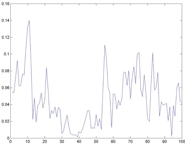
In order to plot the frequency response, it is used the instruction plot(abs(H)). It is necessary change the scale of X axis to see better the graphic in the frequencies rank between 0 Hz and 100 Hz.

Figure 12: frequency response of the filtered signal

After get the frequency response, it is proceeded to calculate the power spectrum density (PSD) in order to find the alpha power, beta and theta, which are the frequencies ranges used in this thesis. So, it must be created an M-File in Matlab (File/New/M-file) to write the code that is needed.

First, it is necessary to write the code which calculates the power spectrum density (PSD). This is as follows:

[n,s] = size(H); % It creates a matrix with size of H

power = zeros(1,s); % It creates a zero matrix

frequencies=zeros(1,s); % It creates a zero matrix

for i = 1:s

frequencies(i) = i/s*512; power(i) = (abs(H(i)).^2)/s; end

[m, fsize]=size(frequencies); % It creates a matrix with size of frequencies

scaleSize=fsize/2;

scaledFreq = zeros(1,scaleSize); % It creates a zero matrix

scaledPSD = zeros(1,scaleSize); % It creates a zero matrix

for i = 1:scaleSize-1

scaledFreq(i) = frequencies(i); if (i>1 & i<scaleSize-1)

scaledPSD(i) = 2*power(i); else scaledPSD(i) = power(i); end end frequencies = scaledFreq; power = scaledPSD;

And then, following the table from the feature extraction section in the background, it is written the code which calculates the alpha power, beta and theta. This is as follows:

% Feature Extraction

alpha=0; beta=0; theta=0;

for i = 1:scaleSize

if(frequencies(i)>=4 && frequencies(i)<8) theta=theta+power(i);

elseif(frequencies(i)>=8 && frequencies(i)<=12) alpha=alpha+power(i);

elseif(frequencies(i)>12 && frequencies(i)<=31) beta=beta+power(i);

end end

When these values are obtained, the feature extraction is finished. Then these features are classified, and to do this, these are grouped to form the SVM input vectors. This is the next algorithm which is used in this thesis in order to reach our goal.

SUPPORT VECTOR MACHINE

The method of signals lineal classification it is going to use is SVM (Support Vector Machine). SVM is one of the simplest classifiers and its empirical and generalization error is quite poor. SVM is a classify algorithm of binary patrons. The objective is separate each patron to one class. For example, if it has two groups, one with white things and another with black things, the algorithm will try to separate those things in function of their color. SVM builds a hyper plane or set of hyper planes in a dimensional space very high and it can use to classification and regression of signals. This hyper plane is created perpendicularly to points and it has to separate a set of points optimally. An algorithm based in SVM takes a set input data (in SVM a data point is viewed as a dimensional vector) and builds a model which can classify that set of points, which they have been given, in one category or another. SVM is also known as maximum margin classifiers because it is looked for the hyper plane which is further away of points which are nearer than that hyper plane. With a set of training examples (samples) it can label classes and train a SVM to build a model that predicts the class of a new sample.

To calculate the similarity function, it is proceeded as follows:

�

� �

𝑥

⋯ 𝑥

⋮

⋱

⋮

𝑥

⋯ 𝑥

� → �

𝑓

⋮

⋯ …

⋱

⋮

⋮ ⋯ 𝑓

�

The first matrix is the landmark vector and the second one is the features vector. The result is the similarity function as it is said previously.

After calculating the similarity function, it has to calculate the cost function where it is called c to the margin distance separator.

This is the general cost function:

−(𝑦 𝑙𝑜𝑔 ℎ

(𝑥) + (1 − 𝑦) 𝑙𝑜𝑔(1 − ℎ

(𝑥)))

Using the above function, it has to sum all the training examples and it has a term 1/m. After, it has to redefine cost functions, taking values, y = 1 and y = 0. It must redefine cost function:

• When y = 1:

• When y = 0:

The complete SVM cost function is:

𝑚𝑖𝑛_{𝑚 �� 𝑦}1 (𝑖) _{�− 𝑙𝑜𝑔 ℎ} 𝜃�𝑥(𝑖)�� + (1 − 𝑦(𝑖)) ��− 𝑙𝑜𝑔 1 − ℎ𝜃�𝑥(𝑖)��� 𝑚 � + _{2𝑚 � 𝜃}𝜆 𝑗2 𝑛 Figure 13: cost1(z) Figure 14: cost0(z)

It is got:

𝑚𝑖𝑛

_{𝑚 ��𝑦}

1

𝑐𝑜𝑠𝑡

�𝜃

𝑥

� + �1 − 𝑦

�𝑐𝑜𝑠𝑡

�𝜃

𝑥

��

+

_{2𝑚 � 𝜃}

𝜆

Linear SVM

Training data have the next form:

D = {(𝑥

, 𝑦

)│𝑥

𝜖 𝑅

, 𝑦

𝜖 {−1,1} }

Where the yi is either 1 or −1, indicating the class to which the point xi belongs. xi is a p-dimensional real vector.

It must find the maximum margin hyper plane. With the next picture, it can see that.

w · x - b = 0

Where w is the normal vector to the hyper plane (and it is a dot product, this product consists on taking two equal length sequences of numbers and returning a single number [23]).

If the data are linearly separable, it can selected two hyper planes which can separate the data, w · x - b = 1 and w · x - b = -1.

Using geometry, it is found the distance between these two hyper planes. For each i, it can have:

• The first class: w · xi – b ≥ 1 • The second class: w · xi – b ≤ -1

And this can be written as:

yi(w · xi – b) ≥ 1, for all 1 ≤ I ≤ n.

Nonlinear classification

The original hyper plane has a linear classifies, but it is necessary another hyper plane to nonlinear classify, for this reason, it is used kernel function. The kernel function is the way to classify nonlinear data and is explained in the next step. Using the kernel function, the resulting algorithm is similar than the linear classification, the difference is every dot product is replaced by a nonlinear kernel function. Also, using a kernel function, a SVM that operates in infinite dimensional space can be built, for every new data; the kernel function needs to be recomputed (At least, there must exist one pair of {H, ɸ} for any kernel function, in H is represented the dot product of the data) [24].

It is a feature space larger than the hyper plane which is used in linear classify.

In the next figure, it can see how, first it is realized a nonlinear classification and then, the linear classification.

Kernel function

The representation with function kernel is a solution when SVM method cannot be used. The reason for using kernel function is because linear learning machines have computational limits; therefore, in most of applications of the real world it is not possible to use SVM method (because it is a linear classification).

The function kernel projects the information in a characteristics space which is larger and increases the computational capacity of lineal learning machines. The theory can extend to separate surfaces nonlinear by mapping the input points into feature points

F = {𝜑(𝑥)|𝑥 𝜖 𝑋}

𝑥 = {𝑥1, 𝑥2, … , 𝑥𝑛} → 𝜑(𝑥) = {𝜑(𝑥)1, 𝜑(𝑥)2, … , 𝜑(𝑥)𝑛}

There are many kinds of kernel function. The SVM can emulate some well-known classifiers depending on the kernel function that it is chosen.

Kinds of kernel function

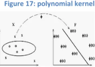
• Polynomial (homogeneous): K(xi, xj) = (xi·xj)n

• Polynomial (inhomogeneous): K(xi, xj) = (xi·xj+1)n • Perceptron: K(xi, xj)= || xi-xj ||

Figure 17: polynomial kernel

• Gaussian radial basis function: separated by a hyper plane in the transformed space: K(xi, xj)=exp(-(xi-xj)2/2(sigma)2).

• Hyperbolic tangent: k(xi,xj) = tanh(kxi·xj+c), for some k>0 and c<0.

Finally, given an algorithm formulated in terms of a positive definite k, kernel can be constructed an alternative algorithm by replacing k by another definite positive kernel

k’.

SVM Multiclass

A multiclass classifier is a function H: X→Y that maps an instance x to an element y of Y. It is focused on a framework that uses classifiers of the form:

𝐻

(𝑥̅) = 𝑎𝑟𝑔 𝑚𝑎𝑥

{𝑀� · 𝑥̅}

where M is a matrix of size k × n over Ʀ and M�r is the rth row of M.

It can be implemented by a matrix of size 2xn, where M� 1 = w and M� 2 = -w, but there is a problem, how it occupies twice the memory needed it is less efficient.

It is necessary to find a good matrix which the empirical error on the sample S will be small and also generalizes well. There is a problem for finding that good matrix because it has to replace the discrete empirical error minimization problem with a quadratic

In general, the sample may not be linearly separable by a multiclass machine, for that reason, it is used this property which is an artifact of the separable case.

To solve the optimization problem is used a double set of variables, one for each restriction. Optimization problem has a solution. This solution is a matrix M whose rows are linear combinations.

Also there is a problem when it is wanted to classify data in two or more categories. To solve that, there are two ways:

1. Each category is divided in other categories and all of them are combined. 2. It is built k(k-1)/2 models where k is the number of categories.

SVR (Support Vector Regression)

SVR is a new version of SVM. The basic idea of SVR consists on mapped of training data to a larger space through a nonlinear mapped where it can realize a lineal regression.

The main characteristic is that SVR is characterized by using kernel. Many of features in machine learning include the use of kernels.

Also, it can apply support vector machine in regression problems. Anyway, it contains all the main features of the maximum margin algorithm. The parameters that are independent of the dimension of the space they control the system capacity.

SVM Properties

SVM has many properties but the most important are:

1. Training a SVM is a convex quadratic programming problem and is attractive for two reasons:

1.1 Its efficient computation.

1.2 The guarantee of finding a global end error surface (it is got a unique solution and most optimal for given training data).

2. It has not the over fitting problem as might occur on Neural Networks. 3. The solution does not depend on the structure of the problem statement. 4. Allows working with nonlinear relationships between data (using function

kernels). The scalar product of transformed vectors can be replaced by the kernel so that it is not necessary to work in space extended.

5. Generalizes very well with few training samples. 6. Linear classifiers.

7. Can be interpreted as an extension of the perceptron.

8. Simultaneously minimize the empirical classification error and maximize the geometric margin.

9. Maximum margin classifiers.

SVM Limitations

Despite the excellent results, the SVM have some limitations:

1. Choosing a suitable kernel is still an open area of research.

2. The temporal and spatial complexity both in training and in the evaluation. It is an unsolved problem with large training datasets.

3. It is far from designing an optimal multiclass classifier based on SVM.

4. The SVM always solves a problem: a change in the training patterns to get a new SVM because it can arise different support vector.

IMPLEMENTATION

First of all, it is necessary to install python and after, it has to download the libraries libsvm-3.17 and SVM_mex601. SVM works in the system, after write the route where is libsvm-3.17, it has to execute the instruction python grid.py -log2c -15,15,0.1 -log2g

15,-15,-The result that it is obtained is 84.44850628946276 3326.985815475168, the first number is the cost and the second one the parameter gamma and the percentage obtained is 56.7308.

After that, it is executed the instruction svm-train. The system shows a list with parameters it can be used.

Usage: svm-train [options] training_set_file [model_file] options:

-s svm_type : set type of SVM (default 0)

0 -- C-SVC (multi-class classification) 1 -- nu-SVC (multi-class classification) 2 -- one-class SVM

3 -- epsilon-SVR (regression) 4 -- nu-SVR (regression)

-t kernel_type : set type of kernel function (default 2) 0 -- linear: u'*v

1 -- polynomial: (gamma*u'*v + coef0)^degree 2 -- radial basis function: exp(-gamma*|u-v|^2) 3 -- sigmoid: tanh(gamma*u'*v + coef0)

4 -- precomputed kernel (kernel values in training_set_file) -d degree : set degree in kernel function (default 3)

-g gamma : set gamma in kernel function (default 1/num_features) -r coef0 : set coef0 in kernel function (default 0)

-c cost : set the parameter C of C-SVC, epsilon-SVR, and nu-SVR (default 1) -n nu : set the parameter nu of nu-SVC, one-class SVM, and nu-SVR (default 0.5) -p epsilon : set the epsilon in loss function of epsilon-SVR (default 0.1)

-m cachesize : set cache memory size in MB (default 100)

-e epsilon : set tolerance of termination criterion (default 0.001)

-h shrinking : whether to use the shrinking heuristics, 0 or 1 (default 1) -b probability_estimates : whether to train a SVC or SVR model for probability estimates, 0 or 1 (default 0)

-wi weight : set the parameter C of class i to weight*C, for C-SVC (default 1) -v n: n-fold cross validation mode

-q : quiet mode (no outputs)

In the command prompt, it has to write svm-train and the name of the file where are every training features. At the end it is added different parameters (mainly parameters –s –t –d –g and –c). Except parameters –c and –g that it has to write values obtained with the function grid.py, all the rest of parameters take its value by default. It is taken values 0 for –s because it is multi-class classification. For the parameter –t takes value 2 (radial basis function) because it returns the optimal result. For –d, the default value is 3. Finally, the value of the parameter –c is 84.44850628946276 and that of –g is 3326.985815475168. So the final instruction which has to execute is: svm-train -c

With the above instruction, it is created the file training.model.txt which it is used in the next step. Now, it is time to use svm-predict.

In the command prompt, it has to write svm-predict training.txt training.txt.model output-training.txt, being output-training the exit file. With this instruction it is got the accuracy. In this case, with parameters previously explained, the accuracy obtained is 88.4615% (it is higher than we expected).

RELATED WORK

In this chapter, research documents and papers, related with this thesis, are explained as follows.

Extraction of Feature Information in EEG Signal

It can get very good results with various time-frequency analysis methods for EEG signal. In addition, it is very difficult that different algorithms used in research documents be useful and it is also complicated integrate them into analysis and EEG detection instrument. With EEG signalsit can detect brain diseases and it can also study the behavior of our brain on many different situations.

In this section, the extraction of feature information in EEG Signal by virtual EEG instrument with functions of time-frequency analysis is explained [7]. In order to be able to make the feature extraction, it converts the EEG signal from time domain to frequency domain, and for this, it is necessary to apply some methods like Fast Fourier Transform or Discrete Wavelet Transform which are explained above. However, in this document is proposed to make the extraction of feature information in EEG signal with functions of time-frequency analysis [7]. For this, it is used the Gabor Transform (GT) which performs an analysis of the signal such that it is able to represent at each time instant, the signal components. It is therefore a time-frequency domain. The definition of EEG signals basic rhythm frequency band relative intensity ratio (BRIR) [14] is used with this function (Gabor Transform) to integrate it into the virtual EEG instrument, because this is the main goal of this research document [7]. Mathematically the Gabor Transform of signal 𝑠(𝜏) is expressed as

𝑔

(𝑓, 𝑡) = � 𝑠(𝜏)𝑔

(𝜏 − 𝑡)𝑒

𝑑𝜏

−∞

𝑔

The discrete Gabor Transform with discrete time and frequency is defined as follows

𝑔

(𝑓, 𝑡) → 𝑔

(𝑚𝐹, 𝑛𝑇)

The sampling interval of time and frequency is represented by T and F respectively. It can see uncertainty in the time-frequency plane when there is a frequency change, because the resolution depends on the size chosen for the analysis window. That is, longer intervals provide good frequency resolution while the narrow windows provide the proper temporary location. Therefore, it has to make a compromise between the time or frequency uncertainty, which depend on each application.

From the Gabor Transform, the spectrum is defined as

𝑆(𝑓, 𝑡) = |𝑔

(𝑓, 𝑡)|

= 𝑔

(𝑓, 𝑡)𝑔

(𝑓, 𝑡)

Slipping output energy and time window as the functions of frequency and time, it can get the time-frequency expression of the signal.

In order to obtain the four classical frequency bands (alpha, beta, theta and delta) in EEG signals, the power spectrum density (PSD) is defined as

𝑃𝑆𝐷

_{= �}

_{𝑆(𝑓, 𝑡) 𝑑𝑓}

(𝑖)_𝑚𝑎𝑥

𝑓(𝑖)_𝑚𝑖𝑛

𝑖 = 𝛼, 𝛽, 𝜃, 𝛿

Where 𝑓(𝑖)_{𝑚𝑎𝑥 and 𝑓}(𝑖)_{𝑚𝑖𝑛 are limits of frequency band i. Therefore, the whole} power spectrum density is

Then, BRIR is defined as

𝐵𝑅𝐼𝑅

(𝑡) = 100

𝑃𝑆𝐷

_{𝑃𝑆𝐷(𝑡)}

(𝑡)

Using BRIR, one of these classical frequency bands is judged by doctors to check whether it is restrained easily in clinical, helping them to do good clinical diagnosis.

In conclusion, there are a lot of parameter feature contained in EEG signals that have relation with some pathological changes, such as sine wave, sharp wave, spike wave, slow wave, etc., so, for this reason, it is very difficult to perform the feature extraction only by a concrete method. Therefore, it is wanted to introduce the virtual EEG instrument with time-frequency analysis functions and these are realized for the feature extraction in EEG signals. Integrating these time-frequency analysis methods into the instruments will advance the performance of EEG instrument.

Sleepiness and health problems in drivers who work driving some kind

of vehicle with nocturnal and shift works

Sleepiness is every time more present in our society, especially on people who are working with nocturnal and shift works. This fact affects more in health of these workers throughout their working life than in health of the rest of workers from other areas that are not related with driving. For example in the document [15], it is explained a study made to railway workers with nocturnal and shift works, where the main goal is to evaluate the health of these workers who are subjected to these work conditions. In this experiment were used as samples 111 men aged between 56 and 38 years old, who work in nocturnal works or in day shifts. The obtained results were analyzed statistically and compared to a group of general working population who works with shift works and these same obtained results were compared to another group of working population who works without shift works. Final results show that railway workers have worse general health state than the rest of workers from other areas, especially presenting big differences in psychic health, in sleep and musculoskeletal pathologies.

Shift work is defined as that one developed by successive groups of people, in which each group plays a workday, so that it is covered a total of between 16 and 24 hours of daily work. This organization [15] supposes the existence of shift work in which the work is done at night, it is to say between 10 pm and 6 am. In today's society, such labor organization is increasing by about 3% a year [16-17].

Workers with nocturnal and shift works go against their physiological circadian rhythms, since they must keep an active vigil when their physiological rhythms induce them to sleep or vice versa [18]. This represents a risk to the health and welfare of workers that extends outside the workplace as it also affects family and social relationships.

20-30% of workers with nocturnal and shift works leave the system working in the first 2-3 years due to serious health problems [19-20]. To avoid this it should conduct a careful medical monitoring of these workers to detect early signs and symptoms of intolerance to it.

Being the machinists a group of workers with nocturnal and shift works an overall assessment health is made to determine those problems prevalent in this group and be able to implement preventive and control measures over them [15].

As mentioned above, in this study [15] have participated voluntarily 111 railway workers, of male sex, aged between 38 and 56 years old with an average of 46 years old. 94 of them belonged to freight trains and the rest of them belonged to passenger trains [15].

After applying the test of overall health, the obtained data are analyzed and compared to a group of general working population who works with shift works. These same obtained data are compared to another group of working population who works without shift works and results show that in the group of railway workers it is observed a higher rate of sleep disorders than in the rest of workers, both in the form of insomnia as increased sleepiness in the waking hours [15]. This is because the individual's natural rhythm is out of sync and is forced to make a daydream which is often of lower quality and shorter duration, with frequent awakenings originated many times by external conditions.

It has been observed that railway workers get a higher score than the rest of workers from other areas in the questions to assess minor psychiatric problems in the population [15], as the tendency to depression, low self-esteem or decrease in the ability to solve problems.

Regarding gastrointestinal health only found significant differences using nonparametric tests [15]. Gastrointestinal disturbances manifested as heavy digestions, pain and heartburn, constipation or diarrhea [15]. These disorders can eventually lead to chronic gastritis and / or peptic ulcer [15]. In these workers these alterations are usually secondary to the intake of more cold or pre-cooked food and meals at irregular hours. In heart health no significant differences are obtained.

These results are the same when machinists are compared to the group of general working population who works with shift works (for the same age rank and sex), and when such machinists are compared to another group of working population who works without shift works [15].

The own machinists focus their complaints in the field of sleep and in the interference of irregular hours in social and family life.

Figure 22: sleepiness

Figure 24: cases with musculoskeletal symptoms

In conclusion, shift work is confirmed as a risk factor for the health and welfare of workers. In the case of railway workers this factor influences specific aspects of health with increased incidence of sleep disorders, both as drowsiness insomnia, mental disorders and musculoskeletal and gastrointestinal system. Knowing these problems, they may be implemented specific preventive programs that should include both worker training in health issues as medical monitoring aimed at early detection and solution of these pathologies.

SVM Regression Training with SMO

As it is said before, SVM is a kind of classification method which, in this project, is used to classify a dataset. SVM has many qualities but, when is had to use to solve quadratic programming (QP), it has been difficult because it is the only algorithm which is known for years. SVM can be optimized by dividing the QP problem into a many smaller QP problems. These sub problems can have fixed size, with optimizing by decomposing; it can be done with a constant size. Also, it is done an optimization of small problems of QP, because it is minimized the original problem QP. A lot of experimental results show decomposition can be faster than QP [22].

Recently, it was introduced the sequential minimal optimization algorithm (SMO) as an example by decomposition because it used a sub problem of size two and each of one has an analytical solution. To optimize SVM, they proposed other methods but SMO is just the online optimizer which uses the analytical solution and exploits the quadratic form, at the same time. SMO is more effective on dispersed data-sets and faster than linear SVM. However, it can be slow on non-dispersed data sets and on problems which have many support vectors. Regression problems have usually these problems because inputs are non-dispersed real numbers. Due to these limitations, there haven't been many reports of SMO which have been used successfully in this kind of problems.

SVM has included variables for nonlinear kernel functions, regression and other extensions for other problems domain. There are a lot of extensions in the basic SVM framework but it cannot talk about all of them. Only it is going to see the derivation of the objective functions which are necessary to set the framework.

The objective function is optimized through converting it into one dual form where are kept the minimization terms minus the linear constraints multiplied by Lagrange multipliers. Lagrange multipliers are used to optimize quadratic function. They are used to

As it is said before, SMO solves the QP problem decomposing that problem into smaller optimization sub problems with two unknowns. Thus, parameters have an analytical solution avoiding the QP solver. Anyway, SMO makes reference to the dual objective functions although it does not use the QP solver. It is defined the output function of nonlinear SVM, with yi 𝜖 {−1,1} , as follows:

𝑓(𝑥, ∝, 𝑏) = � 𝑦𝑖

∝

𝐾(𝑥

, 𝑥) + 𝑏

Where, K(xi, x) is the underlying kernel function. The dual objective function is:

𝑊(∝) =

1

_{2 � � 𝑦}

𝑦

∝

∝

𝐾�𝑥

, 𝑥

� − � ∝

Where, 0 ≤ ∝𝑖 ≤ 𝐶 ∀𝑖 and ∑𝑙𝑖=1𝑦𝑖 ∝𝑖= 0. It is called C a user defined constant and represents a balance between the approximation error and the model complexity. It is necessary to minimize these functions.

The output of the SVM, after minimizing, is:

𝑓(𝑥, ∝

_{, ∝}

_{, 𝑏) = �(∝}

_{− ∝}

₎

𝐾(𝑥

, 𝑥) + 𝑏

− _{are Lagrange multipliers (positive and negative) which satisfy} that 0 ≤ ∝_𝑖+ _{, ∝}

𝑖 , − _∀

𝑖 𝑎𝑛𝑑 ∝𝑖+ ∝𝑖−= 0, ∀𝑖 .

It is minimized the objective function and the form without constraints is:

�(∝

_{− ∝}

₎

= 0, 0 ≤ ∝

_{, ∝}

_{≤ 𝐶 , ∀}

SMO and regression

As it has commented previously, SMO is an algorithm relatively new for training SVM. SMO consists in two parts: The first part consists on a heuristics set for choosing pairs of Lagrange multipliers to work; the second one consists on the analytical solution to a QP problem of size two.

SMO only is applicable to classification problems. To work on regression problems, it must generalize the analytical solution to the size two QP problems. It thinks is one of the most complete and simplest derivations.

There are, at least, three works that derive for SMO regression rules. These works are different in some aspects from this SMO work and from each other.

Below, it explains briefly these three works:

1. The first one is derived from regression rules of SMO. It uses four Lagrange multipliers, but just two of them form a single composite parameter.

2. In the second one is compressed two Lagrange multipliers into a single parameter. Although this rule and the original are seemed, they are very different because, as it is seen, in the second one is more difficult because it is had to compress two multipliers.

3. Finally, the last one is extended of the first derivation that it is had seen in this chapter. The difference is this last derivation corrects an inefficiency of the first one and is the way in how SMO updates the threshold. In classification was the first time where this inefficiency was identified.

Incremental SVM outputs

In the next point, it is going to talk about the SMO modification to calculate SVM output faster. For example, if it is had a SVM which is used to classify and the output is given by the next equation

It is necessary to calculate the derivatives with respect to x, 𝜆and b: • From _𝜕𝑏∗𝜕 𝑓(𝑥,

𝜆, 𝑏

∑

𝛼

𝑦

= 0

𝜆, 𝑏

w* = ∑ 𝛼

𝑦

𝑥

1. Use the above equation, but it is very slow.

2. Only over the nonzero Lagrange multipliers, it can be realized the sum and, for that, it is necessary to change the equation previously given in this point.

3. Incrementally update the new value with 𝑓𝑖 = 𝑓𝑖∗+ �𝜆𝑗− 𝜆𝑗∗�𝑦𝑗𝑘𝑖𝑗 .

Obviously, the last one is the fastest. Depends on what is needed, it uses the second or the third. It is used the second one when it needs an output which has not been increasing updated. It uses the third one when it has non-bounded multipliers and they are had to update. This method can be improved the updating of outputs when they are needed. It is necessary two queues and a third array. The two queues have to be with maximum sizes, it is to say, equal to the number of Lagrange multipliers. The array is created to store a time stamp for the last updated of a particular output. If the value of a Lagrange multiplier changes, it is stored in the multiplier and in the queues it is stored the changed to b. Thus, the oldest value is overwritten.

It can be calculated the output from its last known value if the number of time steps, from the output to the last actualization, is less than the number of Lagrange multipliers different of zero. However, it is more efficient to use the second method to update the output when there are fewer nonzero Lagrange multipliers.

In conclusion, the main idea of this research document is explain another quality of SVM which is more difficult of realizing. It is explained SMO, another method which is used to optimize SVM because is the best to realize this action. Also, it is shown output functions, before and after minimized and finally, how to get these output functions.