An Individual-based Simulation Approach for Generating a Synthetic Stroke Population

Department of Computer Science and Media Technology

Master Thesis Project 15p, Spring 2020

An Individual-based Simulation Approach for

Generating a Synthetic Stroke Population

By

Abdulrahman Alassadi

Supervisors:

Johan Holmgren, Fabian Lorig

Examiner:

Magnus Johnsson

2

Contact information

Author:

Supervisors:

Malmö University, Department of Computer Science and Media Technology.

Fabian Lorig

E-mail: fabian.lorig@mau.se

Malmö University, Department of Computer Science and Media Technology.

Examiner:

E-mail: magnus.johnsson@mau.se

3

Abstract

The time to treatment plays a major factor in recovery for stroke patients, and simulation techniques can be valuable tools for testing healthcare policies and improving the situation for stroke patients. However, simulation requires individual-level data about stroke patients which cannot be acquired due to patient’s privacy rules. This thesis presents a hybrid simulation model for generating a synthetic population of stroke patients by combining Agent-based and microsimulation modeling. Subsequently, Agent-based simulation is used to estimate the locations where strokes happen. The simulation model is built by conducting the Design Science research method, where the simulation model is built by following a set of steps including data preparation, conceptual model formulation, implementation, and finally running the simulation model. The generated synthetic population size is based on the number of stroke events in a year from a Poisson Point Process and consists of stroke patients along with essential attributes such as age, stroke status, home location, and current location. The simulation output shows that nearly all patients had their stroke while being home, where the traveling factor is insignificant to the stroke locations based on the travel survey data used in this thesis and the assumption that all patients return home at midnight.

Keywords: Agent-based simulation, microsimulation, modeling, synthetic population,

4

Popular science summary

Simulation is a computer application with the focus on imitating a process or a system to gain insights and understanding of its internal operations. It is used in a variety of fields from physics to social science since it allows us to test theories that are either costly, dangerous, or not possible to test in real life. The goal of this thesis is to improve stroke patients’ situation by testing whether it is important to consider whether stroke happens at other places than at home, which can help future research designing better policies within healthcare through simulation. However, simulation requires information about patients that typically cannot be acquired due to privacy regulation. After generating micro-level representations of stroke patients, we simulate the patients traveling patterns and the stroke incidents within a region to capture the locations where strokes happen. These locations can help in reducing the time to treatment and future research for deciding upon the ambulance resources. This will reduce the burden on the patients and their families since the treatment within the first hour may significantly improve the recovery rate after a stroke.

5

Acknowledgement

I would like to express my sincere gratitude to my supervisors Johan Holmgren and Fabian Lorig for their continuous support and encouragement for my thesis study. Their guidance, patience, motivation, and immense knowledge helped me in every aspect of the learning process and writing the report. Secondly, I would like to thank all the teaching staff at Malmö University for the knowledge and experience they shared with us.

Finally, I would like to profoundly thank my family and friends for their encouragement and best wishes during the course of this study.

6

Table of contents

1 Introduction ... 11

1.1 Problem Description ... 12

1.2 Goals and Motivation ... 13

1.3 Research Questions ... 13 1.4 Limitations ... 14 1.5 Thesis Outline ... 15 2 Theoretical Background ... 16 3 Research Method ... 20 4 Related Work ... 24

5 The Simulation Model ... 27

5.1 Problem Definition... 27

5.2 Data Collection and Preparation ... 29

5.2.1 Generating the Non-Homogeneous Poisson Process ... 33

5.3 Modeling Cycle ... 34

5.4 Conceptual Model ... 36

5.5 Pre-Initialization ... 39

5.6 The Simulation ... 39

5.7 Implementation and Simulation Framework ... 41

6 Evaluating the Simulation Model ... 44

7

8 Conclusion and Future Work ... 54

Appendix I: The Source Code for NHPP in R ... 56

Appendix II: The ODD Protocol ... 58

1. Purpose ... 60

2. Entities, State variables, and scales... 60

3. Process overview and scheduling ... 61

4. Design concepts ... 61

5. Initialization ... 62

6. Input ... 64

7. Submodels ... 64

Appendix III: The Simulation Class Diagram... 67

8

List of Figures

FIGURE 1 DISAGGREGATION OF ZONAL DATA TO RASTER DATA ... 25

FIGURE 2 HOSPITALS LOCATIONS IN THE REGION OF SKÅNE ... 28

FIGURE 3 THE TOTAL NUMBER OF STROKES PER HOUR ACCORDING TO THE STROKE DATASET... 28

FIGURE 4 THE MODELING CYCLE ... 35

FIGURE 5 THE CONCEPTUAL MODEL ACTIVITY DIAGRAM ... 38

FIGURE 6 THE DIFFERENCE BETWEEN THE NHPP AND THE REAL DATA STROKE EVENT TIMES ... 47

FIGURE 7 THE DIFFERENCE BETWEEN THE GENERATED AND REAL DATA STROKES PER MUNICIPALITY ... 47

FIGURE 8 THE DIFFERENCE BETWEEN THE GENERATED AND REAL DATA STROKES PER AGE GROUP ... 48

FIGURE 9 TRAVELERS PER HOUR IN LUND CITY FROM THE RVU DATASET ... 48

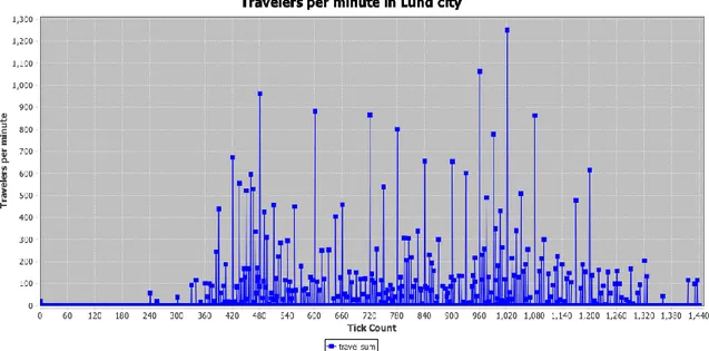
FIGURE 10 TRAVELERS PER MINUTE IN LUND CITY IN THE SIMULATION ... 49

FIGURE 11 TRAVELERS PER HOUR IN LUND CITY IN THE SIMULATION ... 49

FIGURE 12 STROKES LOCATION ... 53

FIGURE 13 THE THREE BLOCKS OF THE ODD PROTOCOL, INCLUDING THEIR RESPECTIVE ELEMENTS ... 59

9

List of Tables

10

List of acronyms

ABM Agent-Based Modeling

ABS Agent-Based Simulation

AIS Acute Ischemic Stroke

DES Discrete-Event Simulation

DeSO Demographical statistics areas (Demografiska

statistikområden)

DS Design Science

IBM Individual-Based Model

MABS Multi-Agent-Based Simulation

NHPP Non-Homogeneous Poisson Process

ODD Overview, Design Concepts, and Details

SAMS Small Areas for Market Statistics

SCB Statistics Sweden (Statistiska centralbyrån)

RVU Travel Habits Survey in Skåne Region

11

1 Introduction

Stroke, a brain attack, is a major cause of disability and the third most common cause of death in western countries [1]. Worldwide, one person out of six is going to have a stroke in their lifetime where 5.8 million will die per year as a result, and the number of deaths can reach 6.7 million annually without implementing appropriate actions [2]. Within seconds to minutes after the occurrence of an Acute Ischemic Stroke (AIS), the brain will experience loss of blood flow in one or more of its regions. This can cause permanent cell damage which compromises the brain functionality, typically leading to some type of disability [3]. The time to treatment plays a major role in preventing permanent brain damage and potential death, where administering intravenous stroke treatment within the first hour results in significant improvements in the recovery rate [4].

A reduced time to treatment will benefit stroke patients to have a higher probability of recovery, where anticipating the locations of stroke incidents enables healthcare management to distribute the ambulance resources more efficiently to provide help more rapidly. To improve the situation for stroke patients, better policies need to be implemented to reduce the time to treatment such as deploying a special type of ambulances for stroke incidents and their placement within the region. However, testing new policies in healthcare systems is usually dangerous since it risks the patients whose health condition is already critical. Therefore, simulation techniques are considered useful tools for gaining insights into situations that cannot be tested in real-life due to complexity, cost, or ethics.

A simulation model is a valuable tool for studying the effect of applying a policy to a population. Simulation is used in different fields such as healthcare, economics, and social studies. Many simulation models require a population of individuals to study. In some cases, a real population is not available to study, it might be necessary to instead develop a synthetic population i.e., microscopic representation of the actual population, where it should include the real population’s structure and dynamics. Researchers and policymakers simulate a population to get understandings of its dynamics and to predict the behavior of

12

large numbers of individuals. An input population, whether it is synthetic or real, is typically needed both in Agent-based and in non-agent-based (micro-level) models.

1.1 Problem Description

The existing simulation projects for stroke-related logistics lack the factor of traveling within the population and considers that strokes happen always at the home location. The locations of stroke incidents presented by Al Fatah et al. [5] is done by simulating random postal addresses of the patients’ locations using the Monte Carlo approach, i.e. the home address of the patient considering a stroke always happens at home, and not on the actual patients’ location at the time of the incident in case of traveling outside their home municipality.

The project idea is to develop a model to generate a synthetic population where its individuals consist of stroke patients including time using demographic statistics, along with their age, home location within one squared kilometer, home municipality, current location, and stroke status. It will be used as an input for an Agent-based simulation to estimate the location of each stroke incident. The modeling approach used is Agent-based modeling, to represent individuals within the region and their travel patterns to capture the location of stroke incidents when occur.

To gain insights about stroke incidents occurring in a region, micro-level simulation approaches can be used to capture the location of stroke incidents. However, micro-level simulation requires data about individuals as input, which is typically not possible to access due to privacy regulations. Therefore, there is a need for generating a synthetic population that represents the actual population in the region, that consists of its individuals that need to be studied, along with their age, gender and location, and their travel patterns throughout the day to be able to capture their location when having a stroke at any point of time. Besides, the number of stroke incidents is required to identify stroke probabilities for each age group.

13

1.2 Goals and Motivation

In Sweden, the total number of stroke patients reached 21895 in 2018 [6]. The treatment within the first hour can reduce the burden on the patients and their families, in addition to the social services where it can save up to 323200 Swedish Crowns per patient [7]. This thesis project aims to incorporate a population of stroke patients in a region based on census data, the density of inhabitants per squared kilometer, and including the locations of individuals within the region. Later, the synthetic population will be used as an input for an Agent-based simulation to estimate the locations of its individuals based on real data that is acquired from a travel survey conducted in 2013, besides assigning strokes to the individuals based on the time of incident generated by a Poisson Process. Since individual-level data is not possible to acquire due to privacy regulations and patients’ integrity, and that is the reason behind the need for a synthetic population of stroke patients by using the available data.

1.3 Research Questions

The main research question is related to the process of modeling and simulation, and the generation of the synthetic population as follows:

RQ: How can micro-level simulation be used to generate a synthetic population of

stroke patientsconsidering travel patterns?

The main purpose of this thesis project is to generate knowledge, which in the long run can contribute to improving the situation of stroke patients, where the goal is to build a model for generating a synthetic stroke population that contains location attributes and takes into consideration the travel patterns of its synthetic individuals. The generated synthetic population can be used in testing stroke-related policies and gaining insights about stroke incidents and their locations, in the long run, helping stroke patients. In addition, we can use the generated model to generate different synthetic populations.

14

The answer to the previous question will provide answers to a set of questions related to the process of microsimulation and agent-based simulation:

1. How can traveling be realistically modeled in the simulation model?

2. How can we distribute stroke incidents on individuals in the simulation model?

1.4 Limitations

There are three main sets of data that is required to build the model, which are census data to get the total number of inhabitants in the region, travel survey data to get the individuals’ traveling patterns, and stroke data to get the total number of stroke incidents in the region. However, the collected datasets were incompatible due to the difference in the date of collecting the data, namely, the census data available for public use was collected in the year 2018, the travel survey was conducted in 2013, and the stroke data is from 2016. The incompatibility is related to the total number of inhabitants in Skåne region in those years, where that difference created a mismatch when generalizing the travel survey sample and the probability of having a stroke since it is based on the number of stroke incidents to the number of people in the region in that year. In some age groups within a municipality, the number of unique travelers generated based on the year 2013 was larger than the actual population in 2018, therefore, several travelers were discarded. Regarding the stroke data, we assumed that the probability of having a stroke is unchanged through the years. Similarly, the travel patterns in an age group are assumed to be the same for the population in 2018.

It is not possible to get the exact location of stroke incidents, therefore, the model needs to predict the location of incidents as accurately as possible. The census data available from SCB provides the number of people living in each squared kilometer in Sweden [8], while the travel survey conducted in 2013 used a different regional division scheme called SAMS and contained up to 46% of missing values for trips details. Due to the difference between partitioning schemes in the two datasets, the location of individuals is in one defined

15

squared kilometer in the grid of the map, or the center of the destination municipality from the travel survey.

Time constraints are the second limitation for this thesis, where the development of complete individual-based simulation is not possible within the allocated time and resources due to the higher complexity of Individuals-based modeling and the need to test other simulation frameworks that are more suitable for the defined scenario.

1.5 Thesis Outline

This master thesis is composed of several chapters. The introduction chapter contains an overview presentation of the thesis, consisting of a brief introduction about the field of study, the idea behind the project, research questions, and limitations. The Theoretical Background chapter provides the reader with the basic knowledge related to the field of study, which is necessary to establish an understanding to readers unfamiliar with simulation and specifically micro-level simulation techniques. The Related Work introduces some methods that are used to generate a synthetic population and its usage in healthcare scenarios. The Research Method chapter describes the research approach conducted in this thesis. Subsequently, the Simulation Model chapter is introduced to present the analysis and the results of conducting the research method for building and evaluating the simulation model. Those findings are examined in the Discussion chapter to further elaborate and analyze the outcome of the thesis, the answers to the research questions, and the threats to validity. Finally, the Conclusion and Future Work chapter is presented to wrap up the thesis work and provide information about future directions for improvements and explorations.

16

2 Theoretical Background

The purpose of simulation modeling is to facilitate two entities; time and behavior, and to state the relationships, events, and effects resulting in the interaction between them. There are two time-advancement mechanisms in simulation: discrete-event and continuous-time. In the Discrete-Event Simulation, the simulation model treats time as a single window or a limited period, while the Continuous-Time Simulation studies the behavior on an uninterrupted period of time.

A model is a purposeful representation of some real system [10]. The reason for building a model is to investigate and solve problems that are not possible to experiment with within the real world, where it can be either expensive to test or it can affect human life. Testing theories in an emergency room environment is an example of a problem field that is not possible to experiment in without a clear indication of its success since it affects patients whose health situation is already critical.

There are multiple simulation paradigms, where each has its own methods of modeling the system under study and the time advancement concept, such as Microsimulation (micro-level simulation), Macro-simulation, Meso-simulation, and Agent-based simulation (ABS). A Microsimulation model represents individuals explicitly as entities in the simulation model, while Meso-simulation models typically groups individuals into groups that are modeled as individuals in the model. The Macro-simulation model makes use of aggregated simulation data. In Agent-based models (ABM), at least one of the “Simulation is a set of techniques for using computers to imitate or simulate the operations of various kinds of real-time facilities or processes” [9]. It is one of the most popular choices in operations research and management science, where it can provide valuable insights on cases where the implementation is costly and time-consuming, such as building a large machine in a factory to improve the production process with no evidence if it is going to achieve the anticipated outcomes [9].

17

modeled entities is an agent. ABM can operate both on micro and meso levels, but typically micro. Furthermore, Discrete-Event Simulation (DES) and Continuous-Time simulation modeling approaches can be applied to both agent-based and non-agent-based models, for example, a DES model can be both micro/meso and both agent-based and non-agent-based.

Microsimulation is a modeling approach for simulating the state and behavior of individual entities such as persons or households [11]. It is usually used in fields related to economics such as unemployment benefits and pensions. However, it is been increasingly utilized in social sciences and demography for predicting future population changes and the impact of policy changes, where experiments in real populations are expensive or unethical. The popularity of the microsimulation approach in demography comes from its capability to model micro-entities explicitly representing a person or a household, which is based on micro-level data that is generated from disaggregating publicly accessed population census or questionnaire surveys. There are three categories of microsimulation models: static, dynamic, and behavioral. These categories are determined based on the characteristics of the created micro-entities, wherein static models, the micro-entity attributes, for example, age, address, and income stay constant through the simulation time, while the dynamic model considers updating the micro-entities attributes through time [12]. The behavioral model includes the individual’s preferences and behavioral traits to study the micro-entity choices and reactions to policy or environmental changes.

Microsimulation models and all simulation models are data-driven in the sense that they require input data, where the properties and behavioral traits of individuals are created by extracting the desired information from census and sample data. In contrast to Agent-based models, microsimulation models do not provide communication between the micro-entities (individuals). Due to that, it is only possible to get the impact of the policy on the individuals and not the other way around [13].

18

While microsimulation models focus on representing population dynamics at the individuals’ level, agent-based models typically focus to a large extent on the interaction between individuals instead, to gain insights about the outcome of unexpected interactions (or emergence) among agents [14]. Furthermore, what characterizes agent-based modeling from other modeling approaches is that it describes the behavior of individuals (agents) in the system, where it is most suitable for modeling scenarios that require a high degree of distribution and localization which is ruled by discrete decisions [15].

An Agent-based simulation is a microsimulation approach that gained more attraction with the rise of computational power in the last decade. In comparison to other simulation approaches, ABS has multiple advantages in modeling and simulating the interactions of entities and the real-world complex systems due to its ability to model pro-active behavior that gives the simulated entities additional dimensions and giving the agents the ability to communicate with each other using a common language since each agent has its thread of execution [15].

There is no exact definition for “agent” that is commonly agreed upon, where agents in the context of Multi-Agent-Based Simulation (MABS) are ranged in characteristics from reactive entities (objects) to fully proactive agents. The characteristics of agents are not completely separated from each other and are identified according to the degree of autonomousity, inter-communication, notions of space, mobility, adaptivity, and mentalistic concepts.

One definition of an agent is “A computer system that is situated in some environment, and that is capable of autonomous action in this environment to meet its design objectives” [16]. An agent-based simulation is a type of behavior simulation that focuses on modeling the behaviors and relations of a group of autonomous agents to capture the followed interaction between the agents, with the system, or with the environment being created in [17]. The interaction between agents can influence the applied policy and even the environment in a bottom-up approach.

19

The strength of microsimulation modeling is in its ability to include rich details about individuals’ characteristics and behavior from census data and population statistics, while Agent-based modeling strength comes from providing the ability of interaction between agents. Combining both modeling approaches will produce a hybrid modeling approach called Individual-based modeling (IBM) which provides valuable insights into population dynamics study and flexibility in modeling heterogeneous populations [14].

Individual-based modeling is used in scenarios that require micro-level data about population’s individuals and being autonomous with interaction capabilities, such as, the spread of disease [18], the impact of transport policies [19], and household demography [20], where synthetic population generation is a necessity for such scenarios and it varies in complexity and structure based on the problem definition and requirements.

20

3 Research Method

The motivation behind the choice of using the DS as the method is strongly related to the aim of this thesis, where the desired result is a simulation model (an artifact), and the generated knowledge expected is how the model should be constructed and the method of generating the synthetic population. On the other hand, the Case Study research method for example focuses on questions related to the behavior of a phenomenon and not on creating a solution for a problem in the form of an effective artifact [23].

There are four types of DS artifacts: constructs, models, methods, and implementations [22], where DS research must create a feasible artifact in the form of these four types [21]. The basic language description blocks for defining problems and solutions are the constructs, while the model is a collection of constructs forming a higher-level description of a process and representing a real-world situation. The method is the process of developing an approach and present guidance to solve the identified problem, and finally, the implementation which is the process of implementing new functionality in the system for a specific purpose [21][22].

Design Science involves two main activities to create an artifact: building and evaluation [22]. The process of constructing an artifact is the building activity, which aims to design and construct the artifact to solve the identified problem, and the second activity The research method conducted for this thesis project is the Design Science (DS) method, which focuses on solving the identified problem by creating an artifact and evaluating its correctness and performance for that objective [21]. The purpose of DS is to create artifacts that help humans reach objectives, and since it is a technology-oriented method, the main criteria for evaluating the created artifact is related to its benefit and efficiency [22]. In contrary to natural science which focuses on creating theoretical knowledge, the DS method concentrates on creating and utilizing knowledge for developing efficient artifacts.

21

is evaluating the artifact’s efficiency and performance as a solution for the identified problem.

The process of Design Science consists of the previous two activities, build, and evaluate, however, Cole et al. [24] and Henver et al. [21] insist on identifying the need for the artifact by showing its importance and relevance to the defined problem field, where developing an artifact must provide an effective solution. Also, Henver et al. emphasize the need for communicating the created artifact with an audience of practicing experts in the field to communicate and review the artifact’s importance, utility, and effectiveness to the identified problem.

A set of DS research criteria is presented by Henver et al. [21] as research guidelines listed in Table 1. The DS research involves the creation of a useful and innovative artifact for a defined problem field, where its usefulness is determined upon evaluation. The artifact must be innovative, intended to solve a currently unsolved problem, or improving the current solution for a known problem in terms of efficiency and performance. The created artifact must be strictly well-defined, represented in a formal method, and consistent in functionality. In addition, the creation of the artifact creates a problem field where the search for the solution utilizes the existing methods and resources to reach the desired results. Finally, the completed artifact must be introduced and communicated with an audience of experts in the problem field.

22

Table 1 Design-Science Research Guidelines [21]

Guideline Description

Guideline 1: Design as an Artifact

Design-science research must produce a viable artifact in the form of a construct, a model, a method, or an instantiation.

Guideline 2: Problem Relevance The objective of design-science research is to develop technology-based solutions to important and relevant business problems.

Guideline 3: Design Evaluation The utility, quality, and efficacy of a design artifact must be rigorously demonstrated via well-executed evaluation methods.

Guideline 4: Research Contributions

Effective design-science research must provide clear and verifiable contributions in the areas of the design artifact, design foundations, and/or design methodologies.

Guideline 5: Research Rigor Design-science research relies upon the application of rigorous methods in both the construction and evaluation of the design artifact.

Guideline 6: Design as a Search Process

The search for an effective artifact requires utilizing available means to reach desired ends while satisfying laws in the problem environment.

Guideline 7: Communication of Research

Design-science research must be presented effectively both to technology-oriented as well as management-oriented audiences.

23

Micro-level simulation models need micro-level data about the modeled individuals, therefore, quantitative data which is expressed in numbers is needed, such as census and survey questionnaires data. The available data about the population in Skåne is collected by Statistics Sweden (SCB) and can be acquired from their website, while the individuals' travel patterns data in the form of a travel survey is acquired from Region Skåne. The travel survey is generalizable where weighting values are included to predict the whole population’s travel behavior. Finally, stroke data is acquired from the Southern Regional Health Care Committee of Sweden, where the dataset provides the total number of stroke incidents in the southern region of Sweden, in addition to the number of strokes for each municipality and at each hour of the day.

In addition to the DS method, a guide for modeling a population for simulation is followed to organize the steps for defining constructs and formulating the conceptual model [25].

24

4 Related Work

Microsimulation is an approach for modeling discrete individual entities, by using micro-level data for describing each entity. It is concerned about studying systems, where a consequence is that large datasets are typically generated from statistical samples and surveys, and estimating the attributes of the individuals within the system based on that data [26]. It is the opposite of macrosimulation techniques that are usually established on mathematical models and focuses on the average characteristics of the population.

Micro-level data for a population’s individuals is typically not possible to acquire due to privacy constraints, and since it is needed for microsimulation, micro-data is acquired as an alternative from the aggregate data that is publicly accessible. The generated synthetic micro-data, i.e., the synthetic population, should be statistically equivalent to the real population, including the individuals’ characteristics in that population, such as age, gender, and location [27].

There are multiple methods for generating a synthetic population, for example, Iterative Proportional Fitting (IPF), Monte Carlo sampling, and disaggregation of zonal data to raster data. IPF is applied to one-dimensional input data from census tracts or statistical areas, to reform it to multi-dimensional distributions which are needed for generating the synthetic population [28]. IPF is dependent on the quality of the input data, and when there is a zero-cell value, IPF must set all zero-cell-values to 0.1 or 0.01, which can affect probabilities and thus the output. Monte Carlo sampling compensates for the mentioned drawback of IPF since it can generate virtually a near to an infinite number of distinct features and allow sampling from one-dimensional distribution to create synthetic multi-dimensional data [29]. The third method for generating synthetic populations is through disaggregating spatial data [30]. Microsimulation models that are based on activities, such as transportation models, need the exact location of the activity, and that is where GIS can be used when micro-data is unavailable. A district’s spatial representation including its aggregated data can be split into raster cells that represent addresses in that district as

25

shown in Figure 1. The land-use distribution is utilized to estimate the density of the inhabitants within that area of different population densities, where initially, the raster representation of the area is generated, and then, the data is distributed to raster cells [31].

Figure 1 Disaggregation of zonal data to raster data [31]

In healthcare scenarios, synthetic population generation is used to create synthetic health records and clinical data since freely available health records are typically not accessible due to privacy issues. The lack of open health records stalled innovation opportunities within healthcare sectors. Therefore, a synthetic population is considered a valuable testbed for researchers to test newer healthcare policies, in addition to allowing industrial and educational parties to contribute to improving healthcare services [32]. Another purpose for generating a synthetic population is to study diseases to implement better prevention and intervention strategies, where spatial data about individuals play a major role in the event of a disease outbreak or an epidemic [33] [34] [35].

A synthetic population of American Samoa is developed based on population census, household data, surveys, and land use geo-data to be used in an Agent-based model with the purpose to capture demographical changes and the heterogeneity of parasitic disease transmission [36]. The hierarchical social structure is important in the study of infectious diseases, where the movements of individuals within the households and region are a main factor in the disease transmission study. The synthetic population contained the main dynamics of the real population such as age, gender, birth, death, marriage, separation, and

26

immigration, where the main focus is to generate a synthetic population as realistic as possible. The output of the simulation showed that the data acquired from the U.S. Census Bureau is either overestimating or underestimating the number of people in certain age groups which was validated against additional datasets from other sources. The generated synthetic population enabled the researchers to understand the real population dynamics and can be used in future studies related to different types of transmissive diseases such as Chikungunya and Zika.

An additional scenario where a synthetic population is needed is shown by Al Fatah et. al. [5], where they wanted a population of stroke patients in the southern region of Sweden as an input for their Agent-based simulation. The simulation purpose is to assess the prehospital triage policies regarding the transportation of stroke patients after the incident. Since patient-level data typically cannot be acquired due to privacy constraints, the population synthesis is constructed using aggregated stroke patient’s data and the Monte Carlo sampling for generating patients address using postal data from the southern region of Sweden, then randomly selecting an address within the municipality of the patient. The main attributes of the generated synthetic population are the patient's age, address, the incident’s time, and the type of stroke.

A synthetic population generation can also be used to assess a community’s health risk due to environmental factors, where micro-level data is produced for the population of New Bedford to study its low-income population exposure to chemicals within the region [37]. The generated population is constructed using census data and includes attributes such as age, gender, education level, and income. In addition, the researchers predict smoking patterns in the population using a multivariable regression method. The geographical locations of individuals play a major role in the study of exposure to environmental risks and the demographical changes that are strongly associated with smoking behavior within the population in low-income areas. The produced synthetic population can be used to assess the community health risks and providing insights into the patterns of vulnerability within the population.

27

5 The Simulation Model

Starting with constructs’ definitions that are done by defining the existing problem with simulation projects for hospital logistics and the need for population dynamicity to include a closer behavior to an actual population. The population representation (model) is introduced in the conceptual model section, where the constructs are combined to form an abstract overview of the studied population. The practices of building the model, in addition to the model description are presented in the modeling cycle section, the final model is described using a standard protocol, and finally, the implementation of the model in a computer simulation is presented and discussed.

5.1 Problem Definition

In addition to the problem description that was stated at the beginning of this thesis, the current simulation models related to stroke patients lack a dynamic location attribute specifying the current location of stroke patients and their travelling patterns.

The system under study is the population of the Skåne region focusing on their travel behavior and stroke incidents. According to Statistics Sweden (SCB), the number of the region’s inhabitants is 1359800 in 2018. The region of Skåne is divided into 33 municipalities and is located in the southern part of Sweden. The population can normally travel within the region, where the travel patterns of individuals are studied by Region Skåne by conducting a survey in 2013.

Hospitals in Skåne region are located in 10 cities and offer healthcare services to the whole region as seen in Figure 2. In Skåne, 3336 stroke incidents happened in 2016, where In this section, I present the solution for the previously described problem, specifically, I describe the artifact, i.e., the simulation model, and its development process by following the DS method presented in the Research Method section.

28

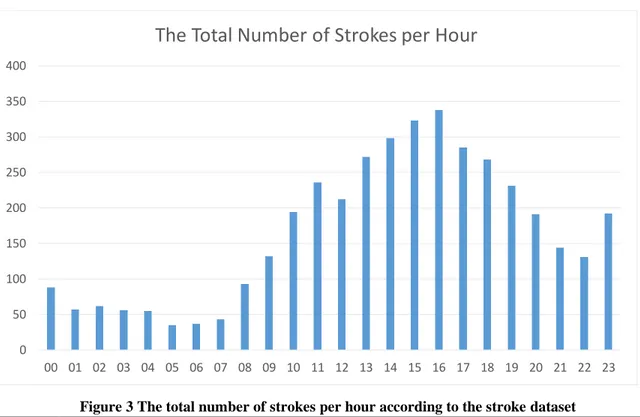
it largely occurs to individuals aging from 45 years old. Additionally, according to the acquired stroke data, the number of strokes is not distributed randomly between the hours in a day, where the probability of having a stroke increases between 10 AM and 9 PM as seen in Figure 3.

Figure 2 Hospitals locations in the region of Skåne

Figure 3 The total number of strokes per hour according to the stroke dataset

0 50 100 150 200 250 300 350 400 00 01 02 03 04 05 06 07 08 09 10 11 12 13 14 15 16 17 18 19 20 21 22 23

29

Recognizing this as a potential place for improvement, I want to contribute to making future simulation projects perform better by generating a synthetic population that represents the stroke population in Skåne region and including the travel patterns of its individuals.

5.2 Data Collection and Preparation

Travel data is needed to know where the individuals travel in the region, and to be able to assume an individual’s location at a certain point in time, while the population data is needed to get information about the whole population regardless if they travel or not. Population data provides information about the density of inhabitants in each squared kilometer, in addition to the age, gender, and the municipality they live in. Finally, the stroke data is required to know the number of stroke incidents per age group and detect patterns in data to know which are more likely to get a stroke and at what time of the day.

A travel survey in Skåne region (Resvaneundersökning i skåne, RVU) was conducted in 2013, to get information about the traveling habits of the population in Skåne region. The survey outcome consists of two sample files, where one contains trip information and the other contains information about the individuals taking the trips. The trips file contains 61 columns and withholds information about trips such as, the person’s ID who took the trip, starting point, destination, trip length, etc. While the individuals' file, consists of 72 columns and contains detailed information about the individuals who did the trips, such as, age, gender, home municipality, etc.

In order to generate the traveling individuals, the dataset file was studied and split into multiple smaller files, where each one contains the group of individuals who lives in the There are three main sets of data that are required for the modeling and simulation, the travel survey data, the population data, and the stroke data, where those datasets contain quantitative data in the form of numbers.

30

same municipality. It was checked for missing data and specifically for the required data for the modeling, such as the IDs, age, home municipality, and weighting values for generalizability.

To generate a travel population, multiple initial steps were done to get the required data. The starting time of trip values in the trips file have some values that did not follow the format HH:MM and contained errors in the format, therefore, the starting time was checked cell by cell to ensure the data followed the standard format.

Datasets typically contain missing values, and in this thesis, it is decided to be left empty without substitution and having the original data without interference. Therefore, the trips that did not have a starting time or destination values are discarded and therefore not changing the current locations of individuals whose trip’s starting time is missing.

This dataset is processed to group and split the values according to the municipality name that the person taking the trip is living in. Each row contains the ID of the traveler and a trip ID, along with the weighting estimate which is a multiplier value that reflects the number of expected trips taken in the real population. Weighting adjustments are included in surveys to compensate for the non-received answers, and to make the received values represent the uncovered population [38]. And to generalize the sample, the number of created objects is equal to the integer number of the weighting value.

There is up to 46% of missing data for the Small Areas for Market Statistics (SAMS) locations for the starting point, home location, and destination area, besides, SAMS was substituted by DeSO in 2018 [39], and it was not possible to get SAMS values in the acquired population dataset. Therefore, it is assumed that the individuals’ location when ending a trip is the center of the municipality to which they traveled.

Since the travel data only included people that are traveling, which is a smaller number than the region’s total population. The population data is downloaded from Statistics

31

Sweden (SCB) website to include the whole population in the model with additional detailed information about the individuals, such as the density of inhabitants in each squared kilometer along with their ages, and to get a more accurate location of a stroke incident if it happened to a person that did not travel yet. The density of the population in each squared kilometer is acquired through Geographic Information System (GIS) data provided by SCB under the Open Geodata section [8], where they offer Sweden’s map divided into a grid with the corresponding population in each cell, where the cell size is one squared kilometer. The disaggregation of zonal data mentioned in the Related Work chapter was not needed, where the spatial data provided by SCB contains a vector grid, instead of raster, with the population density in each cell. The smallest block for defining a person’s original location is assumed to be within a single squared kilometer. Since I only want the grid information in Skåne region and specifically the grid in each municipality, additional geospatial data is downloaded that contains the municipality’s borders to match a grid cell to its corresponding municipality. Later, the two files were merged and exported into another file to be processed in a later step.

The stroke data is provided by the Southern Regional Health Care Committee of Sweden for the year 2016, which contained the number of stroke incidents in Skåne region along with the age of patients, their home municipality, and the time of the incident. In addition, they provided the risk probabilities for each age group based on the statistics of the incidents.

The event of stroke incident for one patient is completely independent of other stroke incidents, and the time of the stroke incident is random where we cannot know the exact time or the place of the next stroke incident. There are undoubtedly some factors implying that a certain person has a higher risk of having a stroke, such as age, and medical history, however, obtaining individual-level medical data could not be acquired due to patient integrity and therefore it was exempted from the model and an assumption is made where patients’ stroke risk is only connected to their age.

32

After examining the stroke data, it was noticeable that a larger portion of stroke incidents happen in the afternoon than in the morning, which means that the incidents are neither evenly nor randomly distributed throughout the day, as seen in Figure 3.

The times of stroke incidents are stochastic independent events that happen more often in the afternoons and are related to the age of the patient. To generate random stroke events, a set of stochastic and probabilistic distribution processes are executed.

According to the stroke data, the number of stroke incidents in Skåne region is 3973 incidents in 2016, where approximately 10 stroke incidents occur every day. Stroke incidents is a series of a continuous and independent event, where the average of incidents each day is known, and we can get the average time between two incidents, also, the occurrence of the incident happens more in the afternoon than in the morning. The Poisson Process is chosen as a method for generating the number of strokes in each day, and the time between the incidents which is exponentially distributed. Since stroke incidents happen more in the afternoon, a non-homogeneous Poisson Process (NHPP) is used to imitate the stroke incidents distribution graph curve throughout the day from the real data [41].

The travel survey was conducted in 2013, the stroke data was collected in 2016, and the population data was collected in 2018. There is a mismatch between the dates of each dataset which can result in lower accuracy in the model’s output. There was no possibility to get detailed travel data for 2018 since the 2013 version is the only one provided for the project, similarly with the stroke data. This created an issue when assigning travel IDs to the population, where the population in municipalities slightly changed between the two dates. Therefore, multiple sets of IDs were discarded in the initialization phase since the number of an age group in a municipality is smaller than the number of travelers within that age group and municipality in 2013.

33

5.2.1 Generating the Non-Homogeneous Poisson Process

There are three sets of methods for generating pseudorandom numbers from a non-homogeneous Poisson Process: inversion methods, order-statistics methods, and acceptance-rejection methods [40]. A method from acceptance-rejection called the thinning is the most prevalent approach for generating NHPP event times [41], where supposing that T1, T2,…,Tn are random variables being the event times of a NHPP with the

rate function λu(t) in the interval [0,t0]. Let λ(t) be a rate function for a time segment t ∈ [0, t0] such that 0 ≤ λ(t) ≤ λu(t). The event times represents a NHPP with rate function λ(t) in

the defined interval if the ith _{event time 𝑇}

𝑖∗ is independently deleted with probability 1 −

λ(t)/λu(t) for i = 1, 2, . . . , n. The following pseudocode represents a thinning algorithm for

generating random variates from a NHPP [40].

Initialize 𝑡 = 0. Generate 𝑢1 ∼ 𝑈(0,1). Set 𝑡 ← 𝑡 − 1 λ𝑢𝑙𝑜𝑔 𝑢1 . Generate u₂ ∼ 𝑈(0, 1) independent of 𝑢₁. If 𝑢₂≤ λ(t) λ_𝑢 then deliver 𝑡. Goto Step (1).

The thinning algorithm [41] is translated into a program function in R language that takes three parameters, the starting time, the end time, and the intensity function λ(t), which takes a time value and returns the intensity (rate) of events in that time value, where the sum of all values is equal to the lambda value of the Poisson Distribution for one day. The source code for the NHPP events generator can be found in the appendix.

34

The rate is measured by calculating the average number of strokes per day to the number of hours in a day, while the number of events is the average number of strokes in the day. The intensity function is created by specifying the probability of having a stroke in each hour to the number of total strokes per day and returning the probability value between 0 and 1. Each event time return is treated as a percentage of a 24-hour value to get the time in the 24-hour range, and then, I ran the event generation function in a loop with 365 runs in order to get the event times for a whole year, where the output is saved and ready to be relocated to the simulation source folder for the stroke generation process.

5.3 Modeling Cycle

Formulating a model for an existing system must be based on our understanding and empirical knowledge of the system and the processes within it. Therefore, studying the system is the main requirement before modeling it, and it starts with formulating questions about the system. It is important to form clear questions about the system since it guides designing the model.

Due to the different dates in which the data was collected, an assumption is made to consider the travel behavior of individuals in an age group is unchanged, also the risk and probability of having a stroke in 2016 are the same for the year 2018.

The model building process is an iterative process, which can be portraited as a cycle of connected processes starting with formulating the question, assembling hypotheses, choosing a model structure and implementing it, analyzing the model, and finally repeat the cycle if the model analysis indicated a need for additional details or modifications, as seen in Figure 4.

35

Figure 4 The modeling cycle [42]

In this thesis project, multiple questions were formed to understand the system at hand. Initially, the questions formulated were regarding the population, like what are the characteristics in the population that are required to know which individuals may have a higher risk of stroke, and what is the travel behavior of the population. These questions indicated what data is required for the model, and how to organize it in order to get insights into the studied population. Medical history and conditions also play an important role in increasing the risk of having a stroke, however, obtaining micro-level data about individuals’ medical history is not possible for this project and considered to be out of the scope and I only tied the risk of having a stroke to the age of the individual.

The model structure is designed based on the essential factors of the studied problem, starting with; the required data and input for the model, the processes, and finally expected output. The model's main input is population data, travel patterns, and stroke probability.

36

The processes are mainly regarding moving the individuals within the region based on the travel patterns and generating a stroke incident based on the probability of having a stroke for an individual within a group of age.

On later iterations, the number of individuals is equal to the number of stroke patients in the region with a traveling pattern that is identical to the traveling data and assigning a stroke randomly to an individual in a group of age based on the stroke data where different age groups have different probabilities of having a stroke. After analyzing the model, there was a need to have a hierarchical command by creating higher entities than individuals in order to have better control over the population. This was done by creating municipality agents, where each one is responsible for processing its sub-population and distributing the load on multiple entities.

Simulating the patient's locations is a simplification of the population traveling patterns on purpose by maintaining the focus of knowing the location of individuals when having a stroke is based strictly on the acquired travel data.

5.4 Conceptual Model

The model category can be either discrete or continuous, and the desired population model is discrete where I want to describe objects as distinctive subjects. The population individuals will be created as separated objects with their characteristics, and when a stroke Conceptual modeling is the second part of the model study after the problem recognition and definition, which mainly focuses on the “What to Model” question. Furthermore, it defines what to study, and it is needed to provide concepts for thinking and communication that will act as a blueprint for the actual modeling process. There are six components necessary to formulate the conceptual model of a population system [25], the model category, conceptual representation, uncertainties about structure and behaviors, the output of interest, the time concept, and the period of interest.

37

occurs, it will affect only one specific person which is chosen randomly from an age group within a random municipality. The model representation is done by defining the attributes and procedures of the individuals. An individual within the population has two types of attributes, constant attributes such as age, gender, home municipality, and original location, while the attributes that will change over time are the current location and the stroke status. The procedures in the model are divided into two main parts: travel and stroke. The travel procedure will change an individual current location from its original place to the destination municipality at the starting time of the trip, where I assume that a trip is completed instantaneously by eliminating the trip duration and the destination is always the center of the municipality due to datasets incompatibility when it comes to the defined area of the trip. The stroke procedure carries the responsibility of assigning a stroke to a random individual at a predetermined time according to a stochastic events generation method.

The desired output from the model is a synthetic population of stroke patients and the stroke incidents that occur within it, which will help in predicting the locations of stroke incidents within the region of focus through simulation. The time concept in the model is a continuous increment of minutes’ quantity and not as a sequence of discrete events. This is decided due to the nature of trips’ starting times which can happen at any minute, and to build a model that can be used with different travel data in the future that can withhold detailed locations according to the new standard of regional division DeSO.

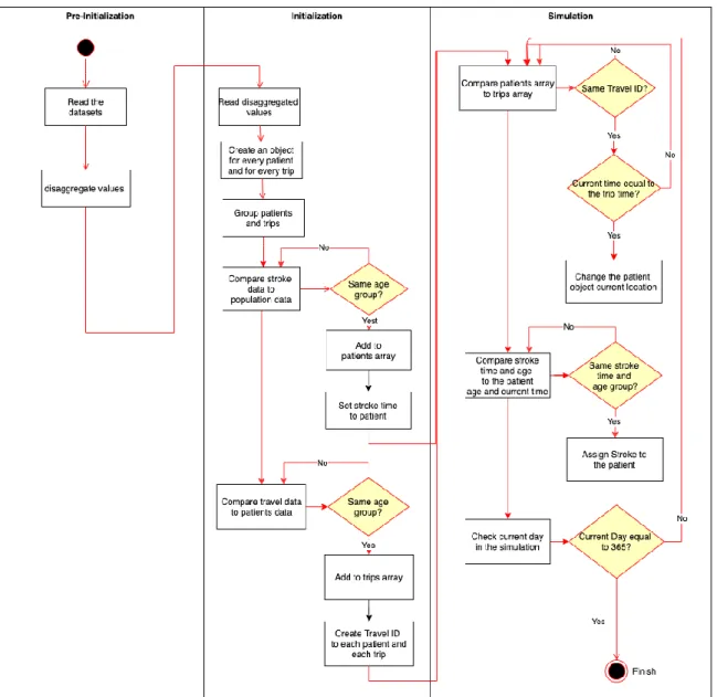
The time period of interest is the year 2018, where the stroke incidents are scattered over that period, however, the travel patterns are repeated weekly since the travel data is a weeklong cycle, based only on the day of the week and lacked the seasonal changes. The conceptual model activity diagram is shown in Figure 5.

38

39

5.5 Pre-Initialization

CSV file format is chosen for storing the data for the simulation, where splitting operations are carried in order to extract and organize the information required for the simulation from the main dataset files, starting with, extracting the data related to the Skåne region from the CSV file that was exported from QGIS.

The first function will go through the population dataset to group the population in the main file into multiple smaller files based on the municipality name and age group. The second function will take the dataset of individuals from the RVU data and group individuals by their home municipality into multiple files. The final function will take the dataset of trips and group the trips by the home municipality of the traveler into multiple files. Additional helper functions are created to validate the newly created files according to the original files.

5.6 The Simulation

Before running the simulation, an initialization phase is needed to prepare the simulation environment and create all the objects that are going to be simulated. After the datasets are disaggregated in the previous step, we create an object for every trip and person, and save them in two different groups (arrays). The array of persons now contains the whole population in the region of Skåne, where we need to create a subset out of it to get only the stroke patients, and to connect the trips to the person that is going to complete those trips. We compare each person in the persons array to the dataset of individuals from RVU dataset to give each one a unique travel ID that is connected to the trips that the person is going to take. The comparison is carried out by going through both arrays and match a person from the persons array with an individual from the RVU dataset based on the age This step is carried to reduce the simulation initialization time, specifically the reading time of dataset files when loading the data and assigning it to the corresponding objects.

40

group and home municipality. After assigning the travel IDs to the individuals, we read the stroke events file that was generated using the NHPP events generator to get the number of stroke patients to be simulated and the time and day of each stroke incident.

The generated number of stroke incidents will be used in two probability mass functions to distribute the strokes on age groups and on municipalities based on the stroke dataset. We later take the samples from both distributions and the stroke events data to create an array of stroke incidents that contains information about stroke age group, municipality, day of the year, and time of occurrence. Finally, we shuffle the persons array and compare it to the stroke objects array to create a subset of the total population that are the stroke patients.

There are two main methods in the simulation, where the first one is changing the current location of stroke patients based on the current tick in the simulation according to the travel data, and the second one is responsible for assigning strokes to the patients at the time of occurrence based on the generated NHPP events.

One tick in the simulation is modeled to be one minute, and to run one year period we need to execute the simulation for 525600 ticks. Starting the simulation will initiate loops to go through the stroke patients’ array and compare each patient’s travel ID to the trip object, finding a match is based on the current tick which can be translated to the time of the day and the date. To assign a stroke to an individual, a loop is going through the stroke objects to compare the stroke occurrence time to the current simulation tick count, and when a match is found, the status of having a stroke is changed in the person object from false to true.

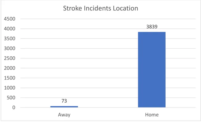
The output of the simulation is collected to be evaluated later, and to get the total number of strokes that happened when a person current location is equal to the original location, i.e., the stroke happened while the patient is at home, and when a person current location

41

is equal to a municipality code which means that the patient had a stroke while being outside his/her home.

The simulation is executed five times and, on each run, the output was collected and saved, where we found that the mean percentage of strokes that happened to the patients while being home is approximately 98.1% of the total stroke incidents, while patients who had a stroke while being outside their home is approximately 1.9%. The simulation model is described in detail using a standard protocol called the ODD Protocol and can be found in the appendix.

5.7 Implementation and Simulation Framework

There is numerous simulation software that offers different features and capabilities for each simulation paradigm and the field of study. Repast Simphony is a popular free and open-source agent-based modeling and simulation toolkit, which can be used on workstations and small computing clusters. It is fully object-oriented with the support for the Java programming language and contains built-in logging and plotting tools, besides, it uses Eclipse as a primary integrated development environment. The architecture of Repast Simphony is designed to maintain rigorous partitioning of the model’s components to provide a modular architecture for easing the model development process, which results in easier model modifications when requirements change [44].

Furthermore, Repast Simphony provides a scheduler that utilizes double precision real numbers for discrete event times and offers the ability to distinguish between events by specifying a priority value for each one.

Methods scheduling is done using annotations which reduces the complexity of calling individual methods for each desired time segment. To run a method periodically at every tick, it is simply done by adding the unconditional scheduling @Schedule annotation before the method declaration code. The Schedule annotation takes a set of parameters to define

42

which tick the method must start executing from, the interval between method runs, and the priority level of the method.

Repast Simphony offers a data collection mechanism to collect and store the information produced by the running simulation. It provides different options for gathering data on an aggregate level, such as sum, mean, and count. Agent’s properties can be also collected using a non-aggregated collection method to capture specific individual values. The data collection system is divided into three parts: data sources, data sets, and data sinks. The data sources part is responsible for capturing the desired information from the simulation while it is running, and the data sink takes the mission of storing that information into an external file or the built-in data viewers. Finally, the data sets contain the definitions of data sources and data sinks.

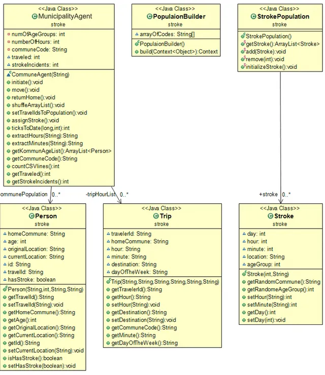
The conceptual model subchapter and the ODD Protocol section in the appendix included the information needed for implementing the model in Repast Simphony using Java. The low- and high-level entities are created as classes, where the properties of these entities are the class’s fields. The MunicipalityAgent class is considered the agent in the simulation environment, where the group of agents that participates in the simulation (the population of agents) are encapsulated in the Context interface. The population builder class is created and it implements the Context interface, where we initialize a MunicipalityAgent for each municipality code and add them to the context. The detailed class diagram of the implementation is shown in the appendix, Figure 14.

Initializing the simulation will trigger the initialization methods mentioned in the Initialization section in the ODD Protocol in the appendix. After the initialization is completed, the simulation can be initiated.

Running the model in Eclipse will open the Repast Simphony simulation window, where we define the data sources, data sets, and charts. The data source type is the custom ContextBuilder implementation that was done in the population builder class. And the data

43

sets are the two functions in the MunicipalityAgent class responsible for returning the number of trips initiated and the number of stroke incidents. The type of the data sets is the aggregated type, specifically the sum, where each data set function returns a numeric value, where the data sets component in Repast sums the returned values from all the MunicipalityAgents included in the context to present the final sum of all trips taken across all agents.

To view the collected data from the data sets component, two charts of the type Time Series are added to the scenario. The purpose of these two charts is to present the number of all trips taken in each tick, additionally, another Time Series chart is created to show the timeline and draw a point for a stroke incident if it occurred at the current tick.

44

6 Evaluating the Simulation Model

The method and implementation parts of the artifact are evaluated against two criteria: performance and efficiency. The main issue realized in the first cycles of implementation was the code complexity of the created functions. The high code complexity made the simulation run extremely slow, which prevented getting the desired insights from the simulation.

A model is a representation of reality, and since we want the model to have realistic travel patterns based on the travel survey, therefore, the simulation output regarding the number of travelers per hour should be collected and compared with the travel dataset.

To validate the travel patterns in the simulation to the real data, the move function is executed more than 2 million times every 1440 tick (a single day in the simulation), to change the current location property of approximately one million objects and to plot the number of travelers in each tick, however, the simulation ran slower in the ticks that correspond to the rush hours in the day (8 AM, and 5 PM), and there was when I noticed that the implemented agents are not running concurrently. Repast Simphony utilized only one core from a multi-core processor, where the agents are not running in parallel on all cores, and as a consequence, simulating one day (1440 ticks) in the simulation would take days to finish (on a machine with 2.4GHz single-core speed). Using the Duration parameter in the method scheduler is said to give the ability to use multi-threading for the simulation [45], however, the method with a duration parameter will run in the background on another thread but will miss the chance of reporting the requested values by the data sets component at the current tick, which will result in not showing the current number of trips at each tick The conducted process of evaluating the artifact is iterative. It started with evaluating the constructs and the conceptual model to define the essential parts of the real system to include in the model and discard the unnecessary factors of the reality, which either cannot be acquired from the existing data or irrelevant to the event of having a stroke.