Implementation Strategies for Time Constraint Monitoring

(1)

Implementation Strategies for Time Constraint Monitoring

(HS-IDA-EA-99-108)

Sanny Gustavsson (a96sangu@ida.his.se)

Institutionen för datavetenskap Högskolan i Skövde, Box 408

(2)

Implementation Strategies for Time Constraint Monitoring

Submitted by Sanny Gustavsson to Högskolan Skövde as a dissertation for the degree of B.Sc., in the Department of Computer Science.

[990618]

I certify that all material in this dissertation which is not my own work has been identified and that no material is included for which a degree has previously been conferred on me.

(3)

Implementation Strategies for Time Constraint Monitoring Sanny Gustavsson (a96sangu@ida.his.se)

Abstract

An event monitor is a part of a real-time system that can be used to check if the system follows the specifications posed on its behavior. This dissertation covers an approach to event monitoring where such specifications (represented by time constraints) are represented by graphs.

Not much work has previously been done on designing and implementing constraint graph-based event monitors. In this work, we focus on presenting an extensible design for such an event monitor. We also evaluate different data structure types (linked lists, dynamic arrays, and static arrays) that can be used for representing the constraint graphs internally. This is done by creating an event monitor implementation, and conducting a number of benchmarks where the time used by the monitor is measured. The result is presented in the form of a design specification and a summary of the benchmark results. Dynamic arrays are found to be the generally most efficient, but advantages and disadvantages of all the data structure types are discussed.

Keywords: Event Monitoring, Real-Time Systems, Time Constraints, Time Constraint Graphs

(4)

1 Introduction

All definitions of a real-time system have at least two things in common – the system must be able to not only deliver the correct results, but also deliver the results at the correct time. Also, real-time systems must be able to detect and react to what happens in the system environment.

These aspects of a real-time system, combined with the fact that real-time systems often operate in environments where uncontrolled or erroneous behavior of the system can have catastrophic consequences, mean that testing and run-time surveillance of the systems are of utmost importance. To facilitate testing and monitoring of real-time systems, tools such as event monitors can be used. An event monitor collects and processes information about the real-time system and its environment, and notifies the real-time system of any interesting results.

This dissertation discusses an event monitoring approach that uses graphs to represent the time constraints posed on the system. A general design for such a system is presented, and different configurations of the design are evaluated. The dissertation is disposed as follows.

Chapter 2 contains a background to real-time systems and event monitoring in general, and the graph-based approach in particular. Chapter 3 formulates the purpose and focus of this project, while chapter 4 describes the method used to reach the project goals. This chapter contains a detailed description of the design for the monitor. Chapter 5 discusses the obtained results, and chapter 6 contains concluding remarks about the project. The three first appendices (A-C) cover details about the event monitor implementation, and Appendix D contains brief discussion on how this work is connected to the theory of science.

(7)

2 Background

This chapter describes the preliminaries to this project, and also defines the concepts which are used in this dissertation. Section 2.1 gives a general description and definition of real-time systems, including relevant categorizations. Section 2.2 covers event monitoring, and defines the key concepts in that area. It also gives examples of areas where event monitoring can be useful. In section 2.3, a brief description of a language that can be used to specify constraints on a real-time system’s behavior is given, and section 2.4 explains how run-time checking of these constraints can be facilitated by using directed weighted graphs to represent the constraints. Section 2.5 presents the objectives that should be attained by an event monitor. Finally, section 2.6 covers algorithm optimization and presents some optimization guidelines.

2.1 Real-time systems

There are several definitions of real-time systems, see for example Kopetz and Veríssimo (1994). The main commonality of all definitions is that a real-time system should not only produce correct results (functional correctness), but also produce these results at the correct time (timeliness). In many cases, real-time systems operate in environments where the inability to execute a task at the correct time could cause great losses, perhaps in the form of damaged equipment, or even human lives. For example, if a space shuttle fails to detach a segment at the correct time during the launch sequence, then the extra weight could mean that the shuttle is unable to exit the atmosphere. This would, in turn, probably result in the death of the shuttle crew and the destruction of billions of dollars worth of equipment.

The need for timeliness implies that all tasks in a real-time system must be predictable and sufficiently efficient. A task is predictable if there is a bound on the amount of resources that the task needs to complete. A task is sufficiently efficient if its resource requirements can be satisfied by the system, and if it is schedulable (i.e., can meet its deadline) given all other tasks in the system.

Real-time systems can be categorized into hard and soft systems (Burns and Wellings 1989), depending on how important it is that the system meets its deadlines, i.e., produces results in time. In a hard real-time system, deadlines must be met, or the system fails completely. In a soft real-time system, a result may be useful even though it was not delivered in time.

2.2 Event monitoring

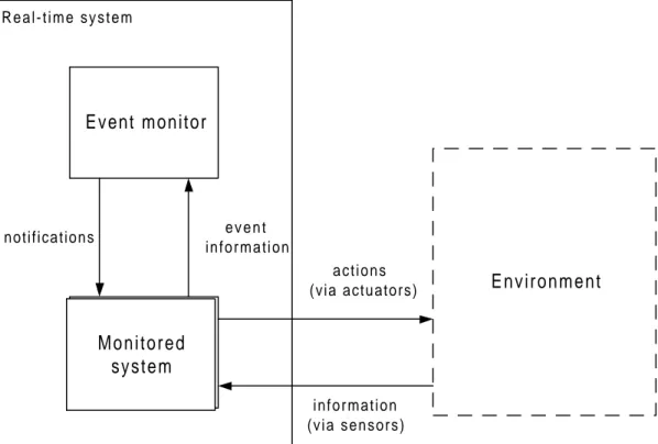
An event monitor provides a way of observing what is actually happening in a real-time system. The monitor collects information about state changes in the system in the form of events. In the approach presented by Liu and Mok (1997a) this information is checked against a set of time constraints (see section 2.2.4) in order to decide whether the system conforms to its specification or not. Figure 2.1 gives a schematic view of a monitored system.

(8)

Figure 2.1: Overview of a monitored real-time system

The monitored system in this figure is the part of the system which interacts with the environment via sensors and actuators. The event monitor gains event information from the monitored system, and returns information (to the monitored system) in the form of notifications. For example, if a violation of a time constraint is detected by the monitor, a notification can be sent to the monitored system which then can take proper actions.

2.2.1 Primitive events

A primitive event can be defined as a change of the system state (Mok and Liu 1997b). According to the definition given by Chakravarthy and Mishra (1993) this state change is atomic i.e., either it happens completely or not at all and happens instantaneously, i.e., has no duration. Moreover, events are only mapped to state changes of interest, since the set of events for a given system would otherwise be arbitrarily large. Events can be defined to occur at, e.g., the start of a transaction, the sending of a message, or the termination of a process.

The difference between the terms event type and event instance should be clarified. An

event instance is what is actually generated when a state change of interest occurs. All

event instances that are generated by the same type of state change (e.g., when a message is sent) are defined to be of the same event type. In this dissertation, the term event is used when referring to ‘primitive event instance’, unless otherwise is stated. Event types are generally recurrent, which means that several instances of an event type can occur during a computation (Mok and Liu, 1997a). An event occurrence is defined by Mok and Liu (1997a) as a point in time at which an instance of an event happens. R e a l - t i m e s y s t e m Event monitor Control unit Environment notifications e v e n t i n f o r m a t i o n i n f o r m a t i o n (via sensors) a c t i o n s (via actuators) M o n i t o r e d system

(9)

Each event type has an event history, which contains the instances of the event type (Chodrow, Jahanian, and Donner, 1991). Event histories are a necessary requirement for run-time monitoring of time constraints, since time constraints can refer to past event instances (further discussed in section 2.2.4). A bound on the length of the history for each event type can be extracted from the time constraint specification (Mok and Liu, 1997a).

2.2.2 Composite events

In the event specification language Snoop (Chakravarthy and Mishra, 1993),

composite events are defined as events that are formed by applying a set of

operators to primitive and composite events. Examples of such operators in Snoop are disjunction (denoted by “∨”) and sequence (denoted by “;”). The composite event (Abort_transaction ∨ End_transaction) occurs when either of the events Abort_transaction or End_transaction occurs. The composite event (Open_file ; Write_to_file ; Close_file) occurs when the event Close_file occurs, provided that the composite event (Open_file ; Write_to_file) has already occurred. Composite events occur when an instance of a terminator event occurs (Chakravarthy et al., 1994). The terminator event is an event that denotes that a composite event has been completed. For example, the terminator of the sequence (Open_file ; Write_to_file ; Close_file) is the event Close_file. The terminator of (Abort_transaction ∨ End_transaction) can be either Abort_transaction or End_transaction. Conversely, the initiator event is the event that starts the composition of a composite event.

2.2.3 Event parameters

Each event type defines a set of event parameters, which are used to hold information related to each instance of the event type. The minimum set of parameters for an event instance is the occurrence time and the event type, since this information is needed to compile an event history for each event type (Chakravarthy and Mishra, 1993). For example, the parameter set for an event of type Car_passed in a traffic surveillance system could include the speed at which the car passed in addition to the time of occurrence and the event type. Each instance of an event type has its own set of values for the event parameters.

2.2.4 Time constraints

Time constraints can be used to specify time limits for the behavior of a real-time system. Time constraints can be in the form of task deadlines (e.g., the air-bag in a car must be inflated within 5µs when a collision is detected) or minimum delays between events (e.g., the WALK light at a zebra crossing should not be lit until at least two seconds have passed since the traffic light turned red). In our work, time constraints are specified using a language defined by Mok and Liu (1997a) which in turn is a refinement of real-time logic (see section 2.3).

2.2.5 Applications for an event monitor

There are two main applications for which an event monitor is useful. Those are (i) testing and debugging of real-time systems (Schütz, 1994) and (ii) supporting fault tolerance in a system (Mellin, 1998).

(10)

Testing and debugging

When testing and debugging a real-time system, timeliness must be considered. In addition, the correctness of an execution in a real-time system depends on what happens in the environment where the system operates during the execution. Thus, a way of observing a system’s internal states is needed. An event monitor simplifies the observation of a system by detecting events and thus allowing event histories to be created during system execution.

If a bug is detected during a test execution, then it is often useful to be able to recreate this execution during subsequent tests to ensure that the bug has been removed. This kind of testing, called regression testing (Adrion, Branstad, and Cherniavsky, 1982), requires a log of the execution to be reproduced. For such a log, event histories can be useful.

Fault tolerance

Laprie et al. (1994) define a fault as a cause of an error, which is intended to be avoided or tolerated. Furthermore, they define fault prevention as the act of preventing a fault occurrence or introduction. This can be compared to error detection and

recovery, which means that error recovery is done after the error has occurred and

been detected.

An event monitor can be used to detect violations and satisfactions of time constraints. If a violation occurs, the monitor can notify the system of the error, and recovery measures can be taken. In some cases, the monitor can also predict future constraint violations, which could be useful for fault prevention.

2.3 Time constraint specification for event monitoring

The language used by Mok and Liu (1997a) to specify time constraints employs two main functions – the event occurrence function (denoted by “@”) and the index

function (denoted by “#”).

Definition 1: For an event e and a positive integer i, the event occurrence function is

defined as

@(e,i) = t

where t is the occurrence time of the i:th instance of event e.

S = Send_message

R = Receive_message

(11)

For example, @(Send_message,3) returns the system time at the third occurrence of the event type Send_message. The most recent occurrence of the specified event is denoted by i=-1, the second most recent occurrence by i=-2 and so forth. An index value of 0 is undefined. Given the event history in figure 2.2, @(Send_message,3) returns 6, since that is the occurrence time of the third instance of the event type Send_message.

Definition 2: For an event e and a time t, the index function is defined as #(e,t) = i

where i is the index of the most recent occurrence of event e at time t. That is,

#( , )e t if t e i if i e i t e i t = 0 < @ ( ,1) ≥ ∧ @ ( , )≤ ∧ @ ( , + ) > ⎧ ⎨ ⎩ 1 1

For example, #(Receive_message,5) returns the index of the last occurrence of the event type Receive_message at time 5. Given the event history in figure 2.2, #(Receive_message,5) returns 1, since the most recent occurrence of Receive_message at time 5 is the first occurrence, which happens at time 4.

The event occurrence function can be extended to represent event occurrences relative to a point in time. This extension is called the relative event occurrence function and is denoted by @r.

Definition 3: For an event e, a time t and an integer i, the relative event occurrence

function is defined as

@r(e,t,i) = @(e,#(e,t) + i) when #(e,t) + i > 0

For positive values of i, this function returns the time for future instances (relative to the specified time). For example, @r(e,5,1) returns the occurrence time of the next

instance of event e at time 5. Given the execution depicted in figure 2.2, @r(Send_message,4,2) returns 6, since #(Send_message,4) = 1 and @(Send_message,

1+2) = @(Send_message,3) = 6. The function call @r(Send_message,@(Receive_

message,2),0) also returns 6, since the most recent event occurrence of the Send_message type at time 7 (the occurrence time of the second instance of Receive_message) happened at time 6.

Given these functions, basic time constraints can be written on the form T1 + D op T2,

where D is an integer constant, op is one of {>, ≥} and T1, T2 are event instance

occurrence times represented by 0 or any of the functions @ and @r. For example, the

constraint @(Begin_transaction,i) + 10 ≥ @(Commit,i) expresses that the Commit event corresponding to a Begin_transaction event must occur within 10 time units. Time constraints are composed by using disjunctions of conjunctions of basic time constraints (i.e., disjunctive normal form). For example, the following time constraint can be used to check that a transaction is either committed or aborted within 10 time units:

(12)

(@(Begin_transaction,i) > 0 ∧ @(Begin_transaction,i) +10 ≥ @(Commit,i)) ∨ (@(Begin_transaction,i) > 0 ∧ @(Begin_transaction,i) +10 ≥ @(Abort,i))

Constraint conjunctions can be optimized by removing unnecessary constraints (Mok and Liu, 1997b), which are constraints that can be removed from a constraint conjunction without affecting the semantics of the conjunction. That is, if a constraint conjunction that contains an unnecessary constraint is violated at a time t, then the same conjunction with the unnecessary constraint removed would still be violated at time t (the same can be said for satisfaction of constraints). Mok and Liu (1997b) describe algorithms for optimizing constraint conjunctions by removing unnecessary constraints.

2.3.1 Expressing composite events with time constraints

The specification language presented in the previous section can also be used to specify composite events, as shown by Liu, Mok, and Konana (1998). However, these specifications differ from those done in, for example, Snoop, since Snoop has a more restricive way of specifying relations between constituents of a composite events. As an example, assume that the composite Snoop event SE = (Receive_message ; Send_message ; Receive_message) should be detected in the execution depicted in figure 2.2. At time 7, the event has occurred. However, it is not clear whether one or two instances of the event has occurred. Furthermore, if only one instance is detected, which of the Send_message instances (at times 5 and 6) should be seen as part of the composite event? In order to increase the expressiveness of Snoop, parameter contexts (Chakravarthy and Mishra, 1993) are used. The purpose of parameter contexts is to dictate when and how a composite event will be generated.

The parameter contexts defined in Snoop are recent, chronicle, continuous, and

cumulative (Chakravarthy and Mishra, 1993):

• Recent: In the recent context, the most recent instance of the composite event’s

initiator event is used for composing the composite event. The composite event SE, for example, would be constructed as (R1 ; S2 ; R2) at time 7, and as (R2 ; S4 ; R3) at

time 9. The event (R1 ; S2 ; R3) is not detected, however, since the event

composition that started with the occurrence of R1 is flushed when the second

instance of the initiator event (R2) occurs. Note also that the event (R1 ; S3 ; R2)

cannot be detected with this context.

• Chronicle: If the chronicle context is used, a composite event is composed of the

first instance of each event type. These instances are then ignored for the purpose of constructing future instances of the event. At time 7, SE would be constructed as (R1 ; S2 ; R2) under the chronicle context, and the next instance of SE would be

(R2 ; S4 ; R3), not (R1 ; S2 ; R3).

• Continuous: Under the continuous context, each instance of an initiator event is

kept track of as a potential composite event. Given the execution depicted in figure 2.2, the composite event CE = ((Send_message ∨ Receive_message) ; Send_message) would be detected twice at time 5 as (S1 ; S2) and (R1 ; S2).

(13)

• Cumulative: In the cumulative context, all instances of each event type in the

composite event are included in the composite event. Under this context, the composite event SE would include both S2 and S3 (R1 ; <S2, S3> ; R2) when it is

detected at time 7.

In order to add a similar expressiveness to real-time logic, Liu, Mok and Konana (1998) extend their specification by introducing two events Es(TC) and Ev(TC), which

occur whenever the time constraint TC is satisfied or violated, respectively. Also, the function occ(e,i) is defined to be true if @(e,i) is defined and @(e,i) ≠ 0. Similarly, the function occr(e,t,i) is defined to be true if @(e,t,i) is defined and @(e,t,i) ≠ 0. Given

these extensions, the recent and chronicle contexts can be represented in real-time logic. Continuous and cumulative context can probably not be represented, and similarly there are expressions in real-time logic that cannot be expressed in Snoop. There are, thus, slight differences in the expressiveness of the two languages. Below, three different translations of the Snoop event (E1 ; E2) are shown as an example

i) (E1 ; E2) ↔ Es(occ(E2,i) ∧ @(E1,-1) < @(E2,i))

ii) (E1 ; E2) ↔ Es(occ(E1,i) ∧ occ(E2,i) ∧ @(E1,i) < @(E2,i))

iii) (E1 ; E2) ↔ Es(occ(E2,i)∧occr(E1, @(E2,i),0)∧@ r(E1, @(E2,i),0)≥@(E2,i-1))

In (i), event (E1 ; E2) occurs whenever an instance of event E2 occurs provided any instance of event E1 has already occurred. This is essentially recent context, given that only one instance of event E1 occurs. In (ii), event (E1 ; E2) occurs whenever the i:th instance of event E2 occurs, provided the i:th instance of E1 has already occurred. This is equivalent to chronicle context. In (iii), event (E1 ; E2) occurs whenever an instance of event E2 occurs, provided an instance of event E1 has occurred at or after the previous occurrence of event E2. To our knowledge, there is no documented way to differ between (ii) and (iii) in Snoop.

2.4 Event monitoring with time constraint graphs

A constraint conjunction can be converted into a constraint graph (Chodrow, Jahanian and Donner, 1991). This kind of directed weighted graph can be used to monitor the constraints that it represents during the run-time of the monitor by instantiating the nodes in the graphs as events occur, and then checking for violated or satisfied constraints.

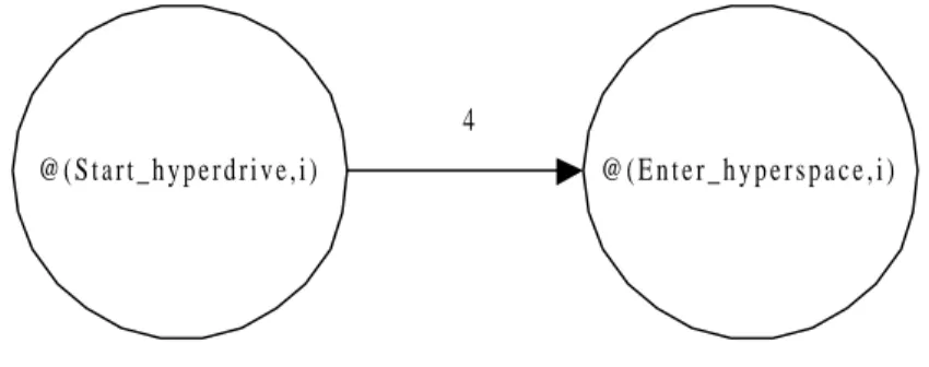
Each basic time constraint is converted into a pair of vertexes connected by a directed, weighted edge. As an example, consider a part of the timing constraint specification for the Millennium Falcon (Lucas, 1977): @(Start_hyperdrive,i)+4≥ @(Enter_hyperspace,i). This basic time constraint, which will be violated whenever the ship fails to enter hyperspace within four time units from the start of the hyperdrive engines (“it’s not fair!”), can be represented by the graph in figure 2.3.

(14)

The weights on the edges in a constraint graph correspond to the integer values in the corresponding time constraints (the D value in T1 + D ≥ T2), and the vertices represent the @- or @r-functions. A vertex that corresponds to a @-function is called

an absolute vertex, and a vertex that represents a @r-function is called a relative vertex

(Mok and Liu, 1997b).

When an event instance occurs, the corresponding vertex in the constraint graph is said to be instantiated, and an occurrence time is associated with that vertex. If both vertices corresponding to the constraint T1 + D ≥ T2 are instantiated, the constraint can be checked for violation or satisfaction by evaluating the inequality.

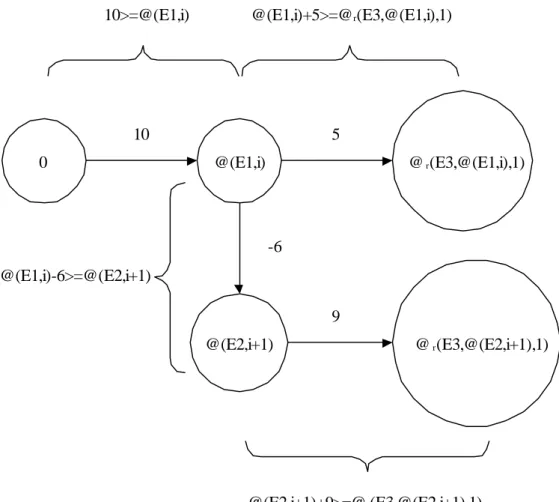
As an extended example, the following constraint conjunction can be represented by the graph in figure 2.4:

@(E1,i) - 6 ≥ @(E2,i + 1) ∧ @(E1,i) + 5 ≥ @r(E3,@(E1,i),1) ∧

@(E2,i + 1) + 9 ≥ @r(E3,@(E2,i + 1),1) ∧ 10 ≥ @(E1,i)

4

@ ( E n t e r _ h y p e r s p a c e , i ) @ ( S t a r t _ h y p e r d r i v e , i )

(15)

The constraint 10≥@(E1,i) is a special kind of basic time constraint, which represents that the occurrence time of the i:th event of type E1 should be less than or equal to 10. A special zero vertex is used to enable representation of constraints of this type.

Constraint graphs are a useful way of representing time constraints, since they facilitate the search for implicit constraints. Implicit constraints are constraints that are not explicitly defined, but that can be derived from the constraint specification. Consider the following constraint conjunction:

@(E1,i) + 1000 ≥ @(E2,i) ∧ @(E2,i) - 999 ≥ @(E3,i)

If the i:th instance of event E1 occurs at time 1 and none of the i:th instances of events E2 or E3 has occurred at time 2, the constraint conjunction above is violated. However, given only the constraints in the conjunction, this violation is not detected until both E2 and E3 has occurred, or at time 1000. The implicit constraint @(E1,i) + 1 ≥ @(E3,i), which can be derived from the constraint conjunction above, will be

0 @(E1,i) @ r(E3,@(E1,i),1) 10 5 @(E2,i+1) @ r(E3,@(E2,i+1),1) -6 9 10>=@(E1,i) @(E1,i)+5>=@r(E3,@(E1,i),1) @(E1,i)-6>=@(E2,i+1) @(E2,i+1)+9>=@r(E3,@(E2,i+1),1)

(16)

violated at time 2. Thus, by finding and including implicit constraints in the constraint graphs, violations can be detected earlier.

2.5 Event monitoring objectives

Regardless of what an event monitor is used for, there are certain properties that are required. Mok and Liu (1997b) present three goals that should be achieved by the monitoring system; transparent monitoring, bounded detection latency, and minimum monitoring overhead. Out of these, transparent monitoring and bounded detection latency are both necessary requirements, while minimum monitoring overhead is a desirable property.

2.5.1 Transparent monitoring

In order to minimize the coupling between the monitoring system and the system being monitored, care should, according to Mok and Liu, be taken to separate the two systems as much as possible. Separating the systems implies that the amount of monitor-specific code in the monitored system should be minimized. Developers of system applications should not need to modify their code to allow their applications to be monitored.

2.5.2 Bounded detection latency

The most important aspect of an event monitor is that it has predictable resource requirements. It is crucial that events are detected within a bounded duration, and that there is a similar bound on the time required to detect that a time constraint has been satisfied or violated and react accordingly. Should no such bounds exist, the monitor loses much of its value, since it cannot be guaranteed that the monitor observes event occurrences in time.

2.5.3 Minimum monitoring overhead

As far as possible, the monitoring system should not affect the execution of the monitored system. This means that the monitoring process should use as little resources as possible, so that the monitored system is not hindered by having to compete with the monitor for processor time, memory, network bandwidth etc. A problem with monitoring a system is that a probe effect (Gait, 1985) can be introduced. The probe effect is the difference in behaivor between a monitored system and its non-monitored counterpart. To avoid this, when monitoring for testing and debugging purposes, the monitor must be left in the operational system (Schütz, 1994). Hence, the overhead of the monitor must be minimized.

The task of minimizing the monitoring overhead can be seen as maximizing the monitor’s efficiency. When improvement of the monitor’s efficiency is an issue, the efficiency and complexity of the algorithms used must be considered. According to Weiss (1999), an algorithm’s complexity is a measurement of how fast the amount of resources needed for the algorithm increases with the number of input values. Generally, the less complex an algorithm is, the better it scales to large numbers of input values.

Algorithm complexity can be divided into time complexity and space complexity. Time complexity is a measure of how fast the time required for an algorithm increases as the number of input values is increased. Space complexity is similar, but is a measure of

(17)

the increase in the amount of resources (such as memory) that the algorithm needs during its execution.

Most of the time, the least complex algorithm for solving a problem is thus also the most efficient one. However, sometimes assumptions can be made about the environment where the algorithm is used that make a more complex algorithm the correct choice. Such an assumption could be an upper bound on the number of input values (for example, events in an event history) to the algorithm. An algorithm with a high complexity could be less time-consuming (more time-efficient) than one with a low complexity when the number of input values to be processed are lower than a given value. If we can assume that our system never requires more values than this to be processed, then we would be advised to use the more complex algorithm (or a hybrid of the two algorithms).

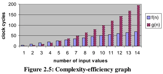
For example, assume that two algorithms, F and G, both take n input values. In figure 2.5, the functions f(n)=5n and g(n)=n2 represent the number of clock cycles needed for F and G, respectively, to produce a result. From the graphs we can see that the time required for F to complete clearly does not increase as rapidly as the time required for G as the number of input values is increased. Thus, F is less complex than G (in the time domain). However, if the number of input values in a system can be assumed to never exceed 5, G will be the most efficient algorithm for that particular system, since the execution time for G is lower than the execution time for F in all situations where the number of input values is lower than 5.

2.6 Algorithm optimization

As discussed in the previous section, the algorithms used by an event monitor must be efficient, especially in terms of computation time. In order to be efficient, the algorithms must be sufficiently optimized. Optimizing an algorithm means that an effort is made to minimize the amount of resources (in time or space) that the algorithm needs. Optimizing a program or algorithm can be facilitated by following certain guidelines. Webber (1992) presents a number of such guidelines, which he refers to as

Figure 2.5: Complexity-efficiency graph

0 50 100 150 200 1 2 3 4 5 6 7 8 9 10 11 12 13 14

number of input v alues

c

lock cycle

s

f(n) g(n)

(18)

the Principle of Least Computations. The essence of this principle is that a computation is unnecessary if

• the result of the computation is already known, or

• the result of the computation is not needed, neither as an output of the program

nor as an input for a future computation

If the program already knows the result of a computation, then the computation can be eliminated. However, this implies that the result is stored, either in memory or on secondary storage. Thus, in decreasing the program’s execution time we also increase the amount of resources it uses. Most of the time, however, processor time is a more limited resource than memory, and the trade-off is justified.

2.7 Existing work on constraint graph-based monitoring

An approach for monitoring of events on a uniprocessor system is described in Mok and Liu (1997b). In this paper, a way of specifying time constraints based on real-time logic is presented. These specification statements can be converted into constraint graphs, and Mok and Liu describes algorithms for (i) deriving implicit time constraints from constraint graphs, (ii) optimizing the graphs for efficient run-time checking of time constraints, and (iii) actually instantiating, updating and checking the graphs as events occur. These concepts are further discussed in chapter 4.

Mok and Liu’s work is based on an approach originally developed by Chodrow, Jahanian and Donner (1991). However, Mok and Liu have improved the approach in several ways. Most importantly, the optimization of the constraint graphs done in Mok and Liu’s method improves the time complexity of the constraint checking algorithms from Ο(n3) to Ο(n), where n relates to the amount of vertexes in the constraint graph.

(19)

3 Problem description

This chapter explains and motivates the project focus, and describes the problems associated with creating a time constraint graph-based event monitoring design.

3.1 Purpose and project focus

The purpose of this project is to provide a flexible event monitor design that can serve as a basis for an implementation of Mok and Liu’s event monitoring approach (1997b, 1998). The design focus is on issues that may have an influence on efficiency, and, in particular, on different methods for representing constraint graphs internally.

3.2 Motivation for efficient event monitoring

No matter for what purpose an event monitor is used, it is important that the monitor is efficient. As described in section 2.2.5 (on pages 6-7), the three main applications for event monitoring are testing, debugging, and fault tolerance. In all of these cases, monitoring efficiency is important. If the extra system load introduced with a monitor in a system is high, it may render a previously schedulable load unschedulable. In such a case, the event monitor is not sufficiently efficient, and as a result the monitored system is not timely.

3.3 Assumptions about monitoring and the monitoring environment

An event monitor can be seen as having an event-collecting part and a constraint-checking part. In this project, the part of the event monitor that handles the collecting of event information from the system, which is system-specific, is not considered. Further, it is assumed that event occurrences are detected instantly by the event monitor.

If the monitor is used in a distributed real-time system, it is also required and assumed that the messages (and thus the events) in the system are stable (Schneider 1994). In short, this means that all events are sent to and processed by the monitor in the order that they occurred. For simplicity, it is also assumed that all events in the network (regardless of which network node they are produced on) are detected instantly and have a correct timestamp based on a global time.

It is also assumed that the system provides sufficient resources for the event monitor to run. For example, there is enough memory to store event histories of the required size and the task load including the monitor is schedulable.

3.4 Using time constraint graphs for efficient event monitoring

As described in section 2.5, an event monitor should be transparent, i.e., there should be no need to introduce monitor-specific code into the monitored system, and predictable, i.e., there should be a bound on the monitor’s resource requirement and efficient. The approach presented by Mok and Liu conforms well to these objectives. If all primitive events in the system can be detected by means of hardware (e.g., by hardware sensors or bus snooping) no monitor-specific code is needed in the monitored system. Thus, transparency can be achieved. Given the assumptions that (i) sufficient resources exist for the monitor to run, (ii) events are stable, and (iii) the time

(20)

Jahanian and Donner (1991)), it is also efficient in terms of algorithm complexity, since the time complexity of the algorithms used during run-time is only Ο(n) with regard to the number of vertices in a given time constraint graph. There are, however, factors that may affect efficiency that are not covered by Mok and Liu, such as the event monitor’s internal representation of the constraint graphs.

3.5 The data storage and representation problem

In an implementation of the event monitoring method presented by Mok and Liu (1997b) there are several places where object relations need to be represented. For example, the event monitor needs to maintain a list of all the constraint graphs that should be monitored. In an object-oriented design (which is used in this project), this could translate to an event monitor object keeping track of several constraint graph objects. The same can be said for the relation between constraint graphs and vertexes, as well as several other relations in the system.

The question is how these relations in general, and the constraint graphs in particular, should be represented in the implementation. The primary problem is what kind of data structure should be used. There are a number of options, each of which has certain advantages and disadvantages. The structure types evaluated in this project are dynamic arrays, static arrays, and linked lists.

(21)

4 Method

In this chapter, the approach taken to handle the issues presented in chapter 3 is presented. In particular, a design based on Mok and Liu’s monitoring approach is described. Sections 4.1 and 4.2 give an overview of the central concepts in the design, while section 4.3 contains a more detailed description of the complete design.

4.1 Design overview

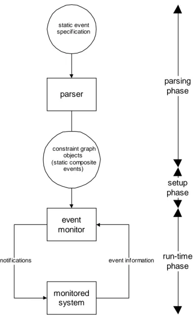
The design consists of two main parts – the parser and the monitor itself. The parser is used during the first phase of execution, which can be referred to as the parsing phase (see figure 4.1). During this phase, the user-specified event types are converted into an internal format. The parsing phase is followed by the setup phase, during which this internal format is loaded by the monitor. During the final phase, the run-time phase, the actual monitoring of the events is done. Also, certain events types can be added to or removed from the monitor during this phase.

static event specification parser constraint graph objects (static composite events) event monitor monitored system

notifications event information

parsing phase run-time phase setup phase

(22)

4.1.1 Central object model

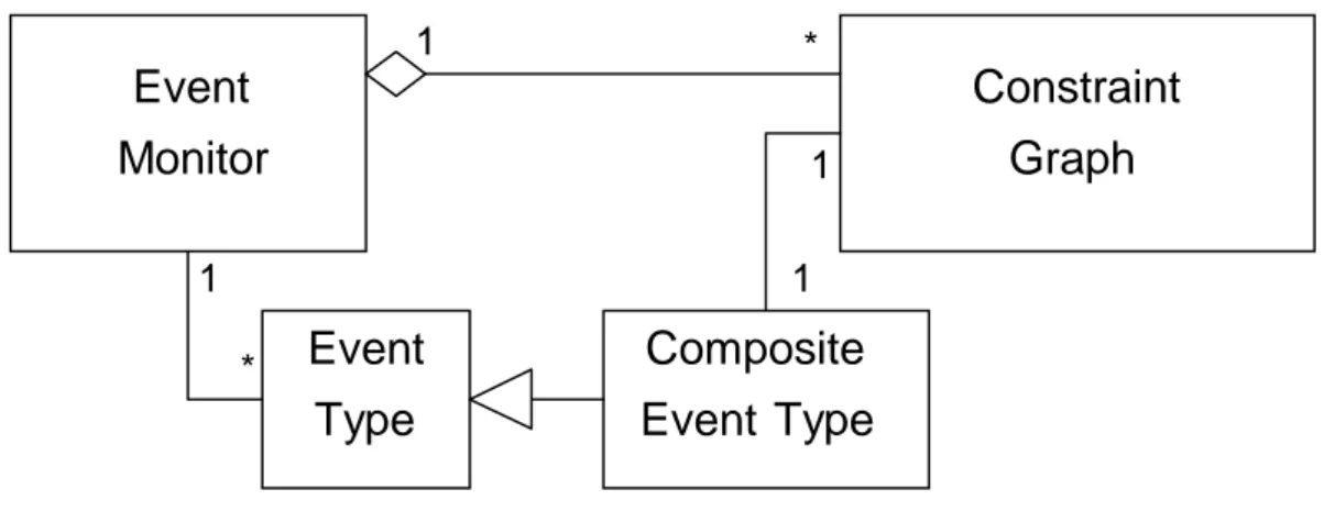
The design presented in this chapter focuses on the representation and handling of constraint graphs. Figure 4.2 shows the relationships between constraint graphs, event types, and the event monitor.

A single, permanent event monitor object exists during the entire monitoring session.

This event monitor object maintains a number of event type objects, which can represent primitive or composite event types. Composite event type objects are associated with a number of constraint graphs that are used to determine when the composite event type has been detected. Instances of the event type, composite event type and constraint graph classes are used as the internal format of the time constraint specification.

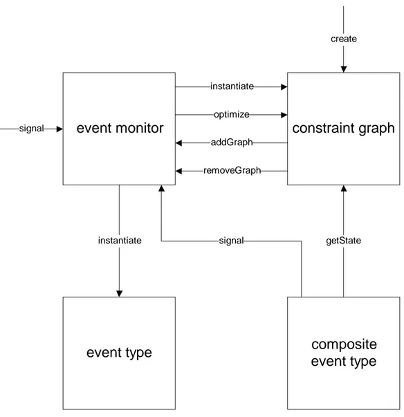
The relation between the event monitor and the constraint graphs in the system is not strictly necessary, since it is a derived relation, but is useful in order to quickly find the relevant graphs when an event occurrence is signaled to the event monitor. Figure 4.3 shows a schematic view of the main collaborations of the central classes

Event

Monitor

Constraint

Graph

Event

Type

1 * 1 *

Composite

Event

Type

1 1

(23)

The event monitor object receives and processes event occurrence signals from the monitored system and from composite event type objects. When such a signal is received, information about the event occurrence is sent to the relevant event type and constraint graph objects via the instantiate interface methods.

When a constraint graph object has been created it adds itself to the event monitor object. If a constraint graph object is removed for any reason, it can also remove itself from the event monitor. The constraint graph interface also contains a getState function, which is used by composite event type objects to find out if the time constraints represented by the constraint graph has been satisfied or violated.

For a detailed description of the class interfaces in the model, see Appendix C.

4.2 Data structure types and object relations

As described in section 3.5, object relations can be represented by different types of data structures. The data structure types that are evaluated in this project are dynamic arrays, static arrays, and linked lists. The properties of each of these are:

event monitor

composite

event type

constraint graph

instantiate optimize addGraph removeGraph getState instantiate signal create signal

(24)

• Dynamic arrays are flexible in size, since the number of slots in the array can be

changed at run-time. This means that no unused memory is ever allocated, as can be the case with static arrays. However, the allocation and deallocation of memory that is necessary to maintain a dynamic array may lead to external memory fragmentation, especially if the arrays are large.

• Static arrays have a fixed size, which means that no new memory has to be

allocated at run-time. The drawback is that the maximum size of the arrays must be predicted at compile time, and if these assumptions are pessimistic a lot of memory is wasted.

• Linked lists are more space-efficient than static arrays with many unused slots.

They are, however, less space-efficient than dynamic arrays, since a pointer to each data entry must also be stored. However, since it is not necessary to store all entries in a linked list linearly in memory (as is the case with arrays), external memory fragmentation is not a concern.

Linked lists allow data to be inserted and removed efficiently with relatively little memory management. However, if a linked list is to be copied, each data entry must be copied individually, resulting in an amount of subroutine calls equal to the number of data entries. If an array is used, the linear storage of data means that all entries can be copied as a single memory block.

4.3 Extended design

In this section, an extension of the basic design described in sections 4.1 and 4.2 is presented.

4.3.1 Event model

For the purposes of this project, events types are separated into static events types and

dynamic event types. Static events types are events types that are specified before the

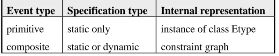
monitor execution is started, and dynamic event types are events types that can be added or removed at run-time. The table in figure 4.4 shows the relation between event types and their representation and specification method.

As can be seen in the table, primitive event types cannot be specified dynamically. It is assumed that all necessary primitive event types are already identified and exist in the system when the monitor is started. This assumption is reasonable in systems that do not allow new elements (e.g., new hardware) to be added to the system during run-time. In a system where such dynamic additions are allowed, new primitive events that are related to the new elements would have to be added to the monitor dynamically. If the presented design is used in such a system, the monitor would have to be restarted each time the set of primitive event types changes.

Event type Specification type Internal representation primitive static only instance of class Etype composite static or dynamic constraint graph

(25)

4.3.2 Event parameter model

In the design presented here, event parameters can only be specified for primitive event types. Composite events are assumed not to have any parameters other than the default parameters (occurrence time, event type) and those that can be derived from its constituents.

4.3.3 The parser and the event specification language

The code for the parser was created using the UNIX programs lex (for tokenizing/keyword recognition) and yacc (for parsing). The parser’s task is to read a specification and generate constraint graph objects (instances of the constraint graph class). These objects are related to one composite event each, and are loaded by the monitor either during the setup phase (for static event types) or during the run-time phase.

Specification of static composite event types

Composite event types are specified using a simple specification language. Figure 4.5 shows the specifications of three different composite events.

a)

event Hyperfail is violation of [

@(Start_hyperdrive,i)+4>=@(Enter_hyperspace,i) ]

b)

event TransactionMetDeadline is satisfaction of [

@(Start_transaction,i)+5>=@(Abort_transaction,i) || @(Start_transaction,i)+5>=@(Commit_transaction,i) ]

c)

event Zebrafail is violation of [

@(Walk_light_off,i)-10>=@(Walk_light_on,i) && @(Walk_light_on,i)+40>=@(Walk_light_on,i+1) ]

(26)

4.5 (a) shows the specification of an event type based on the constraint graph example in figure 2.3 (on page 11). That is, it represents one of the constraints that can be posed on a spaceship hyperdrive. The composite event type in 4.5 (b) could be used to specify that a transaction has met its deadline if it is either aborted or committed within 5 time units. Finally, the composite event type in 4.5 (c) is instantiated if the walk light in a zebra crossing is lit for a duration of less than 10 time units, or if there is a period of more than 40 time units between two occurrences of the event Walk_light_on. “Hyperfail”, “TransactionMetDeadline”, and “Zebrafail” are examples of event names. The event name is a user-specified string that must start with a capital letter and is used as the name of the composite event type. The satisfaction and violation keywords are used to specify whether the event should be signaled on satisfaction or violation, respectively, of the specified time constraint graph. The basic time constraints specified between the square brackets must be written in disjunctive normal form (see the definition of time constraints in section 2.3), separated by “&&” (AND) or “||” (OR). See appendix A for a formal definition of the language in extended Backus-Naur Form (ISO, 1996).

Specification of dynamic composite event types

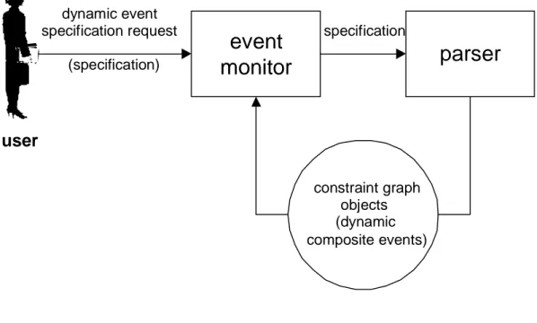
Dynamic composite event types are specified using the same language as static composite event types, and can thus be parsed using the same parser. The difference is that the specification of static composite event types is parsed before the monitor is started, while addition of dynamic composite event types are requested by the user, as shown in figure 4.6.

parser

constraint graph objects (dynamic composite events)

event

monitor

user dynamic event

specification request specification

(specification)

Figure 4.6: Dynamic event specification

When dynamic event types are added, the specification is sent to the event monitor. The monitor invokes the parser, which generates time constraint graphs and composite

(27)

event type objects from the specifications in the file and adds them to the monitor.

Specification of primitive event types

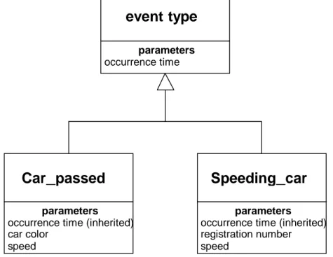
To specify a primitive event type, an object of the event type class is created. Exactly how this is done depends on the programming language used. By modifying the event type class, events types can be modified to contain more parameters than the default parameters. A possible way of specifying different parameter sets for different event types is to use the event type class as a base class for multiple event type subclasses, as shown in figure 4.7.

In this figure, the event type class is the superclass of two event type subclasses that could be used in a traffic surveillance system. The superclass have only one parameter (the occurrence time), which is inherited by the subclasses. However, the subclasses also add certain parameters of their own – car color and speed in the Car_passed subclass, and registration number and speed in the Speeding_car subclass. All parameters of an event type subclass are recorded in the event history of that class. 4.3.4 Complete object model

The object model for the implementation is presented in figure 4.8.

parameters

occurrence time (inherited) car color speed parameters occurrence time

event type

Car_passed

parameters

occurrence time (inherited) registration number speed

Speeding_car

(28)

A short summary of the classes in the model follows:

Event monitor

An event monitor object is the ‘core’ of the implementation. It contains a number of constraint graphs (the monitored graphs) and a table that lists which graphs are associated with a certain event type. This table is used when an event instance occurs in order to determine which constraint graphs should be notified of the occurrence.

Event type

Each direct instance of the event type class represents a primitive event type. It contains an event history which stores the occurrence time and parameters of all instances of this event type.

Composite event type

Each composite event type object is associated with a number of constraint graphs. Constraint graphs represent the signaling rules for the composite event. The composite event type class is a subclass of the event type class, and inherits the properties of that class – most importantly the event histories.

Constraint graph

A constraint graph object contains a number of vertex objects and a number of edge objects. Each connected pair of vertices represents a basic time constraint (see section 2.4 on page 10).

Vertex

A vertex object contains the name of the event type associated with the vertex and an index. The index, which is an arithmetic expression on the form a*i+b (a and b integers, i a variable), is used to determine which instance of the associated event type should be used for instantiation of the vertex.

Event Monitor Constraint Graph E d g e Vertex Timer Deadline Timer Timeout Timer Event T y p e Relative Vertex references 1 * * 1 1 1 * * 1 1 + 1 2 + * * 1 1 f r o m to C o m p o s i t e Event Type 1 1

(29)

Relative vertex

A relative vertex object has the same properties as a vertex object, but adds an association to another vertex object (the reference vertex of the relative vertex).

Edge

Each edge object is associated to two vertex objects, which define the start and end of the edge. It also contains the weight of the edge, which represents the deadline or timeout time for a time constraint (the D value in T1 + D ≥ T2).

Timer

Timer is an abstract superclass of the timeout and deadline timer classes. Each timer object, regardless of type, contains an association to the vertex that the timer notifies whenever a timeout is detected or a deadline is reached. Each vertex controls the creation and termination of all timers that are related to the instantiation of the vertex. Timers are often needed to ensure early detection of constraint violations (Mok and Liu, 1997a).

Assume that a time constraint on the form T1 + D ≥ T2 is monitored, and that the

vertices V1 and V2 are the corresponding vertices to T1 and T2, respectively. If V1 and

V2 are both instantiated, then the constraint can be evaluated. However, if only one

vertex is instantiated, then a timer might be necessary to ensure detection of a constraint violation. The table in figure 4.9 shows the timers needed in a given situation (Mok and Liu, 1997a).

Deadline timer

An instance of a deadline timer object is created whenever a constraint implies a deadline for the instantiation of a vertex once the other vertex in the constraint has been instantiated. If the timed vertex is not instantiated before the timer is finished, the associated constraint has been violated.

Timeout timer

A timeout timer is used when a constraint specifies a necessary delay between the instantiations of two vertexes. If the timed vertex is instantiated before the timeout timer has finished, a violation has occurred.

4.3.6 Program flow

The event monitor is idle as long as there are no event occurrences in the system, but State of V1 State of V2 Value of D State of constraint

not instantiated not instantiated irrelevant cannot be evaluated instantiated not instantiated positive deadline timer needed instantiated not instantiated negative always violated not instantiated instantiated positive always satisfied not instantiated instantiated negative timeout timer needed instantiated instantiated irrelevant can be evaluated

(30)

schematically what happens when the monitored system signals an event occurrence to the event monitor.

When the event monitor receives an event occurrence signal from the monitored system or from a composite event type, it immediately forwards this information to the relevant constraint graphs and the instantiated event type. The event type records the parameters of the instance in its history. Since an event history has a bounded size, this could cause the first history entry to be flushed from the history.

When a constraint graph becomes notified of an event instance, it searches its set of

event

type

event

monitor

monitored

system

composite

event type

constraint

graphs

primitive event occurrence compos ite event occurrence ins tantiation event occurrence information

s atis faction/violation notification

Figure 4.10: Overview of program flow

event

type

event occurrence information event history parameters possible flush

(31)

vertices, and instantiates any matching vertex to the occurrence time of the event instance. If the graph is satisfied or violated as a result of the instantiation, this is signaled to the composite event that the graph is associated to (see figure 4.12).

If this causes the composite event to occur, an event instance of the composite event type is generated, and signaled to the event monitor. The monitor notifies the monitored system of the event occurrence, and the cycle starts over.

Note that some vertices in the graph may contain arithmetic expressions (instead of numerical values) for their index. That is, they may relate to occurrence functions on the form @(Eventname,a*i+b). If such a vertex with a matching event name is found when the graph is being instantiated, the monitor tries to find an integer value for i that satisfies the equation a*i+b = event occurrence index. This is done by setting i=(event occurrence index - b) / a.

If a value for i is found, the constraint graph creates a clone of itself. This clone is a copy of the original constraint graph (and is thus associated with the same composite event type as the original), but all arithmetic index expressions in the cloned vertexes are replaced with their matching numerical values for the computed i value. The constraint graph clone object is added to the monitor, and functions as a regular constraint graph, with the exception that once the clone has been satisfied or violated, it is removed from the system. Consider the following example:

The composite event type ExampleEvent is defined as

constraint

graph

instantiation instantiation and evaluation

composite

event type

satisfaction/violation notification

event

monitor

composite event occurrence

constraint

graph clone

possible creation added to

Figure 4.12: Instantiation of a constraint graph

event ExampleEvent is satisfaction of

[

@(E3,3*i-4)+4>=@(E4,i) && @(E3,3*i-4)-3>=@(E1,2) &&

(32)

This event type is represented by the graph in figure 4.13.

Assume that the second occurrence of the event type E3 is signaled to the event monitor at time 9. The monitor forwards the information to the constraint graph, whose set of vertices is searched for a vertex that matches @(E3,2). No such vertex is found, but by setting i=2, @(E3,3*i-4) would be equivalent to @(E3,2), since 3*2-4=2. Thus, the graph is cloned, and i is replaced with 2 in all vertexes in the cloned graph. The resulting clone is shown in figure 4.14.

Note, that the vertex that is now corresponding to @(E3,2) is immediately instantiated, since it matches the event occurrence that triggered the cloning.

4 @ ( E 4 , i ) @ ( E 3 , 3 * i - 4 ) @ ( E 1 , 2 ) - 3 @ ( E 2 , 2 * i ) 5

Figure 4.13: Constraint graph for ExampleEvent

4 @(E4,2) @(E3,2) (instantiated at time 9) @(E1,2) -3 @(E2,4) 5

(33)

4.3.7 Algorithms

Three algorithms presented by Mok and Liu (1997b) are used in the design presented here. The algorithms and their respective functions are described below. For a complete pseudo-code description of the algorithms, see Mok and Liu (1997b).

Graph compilation

The graph compilation algorithm is used during the setup/parsing phase to remove all unnecessary constraints from a constraint graph, and also to find the shortest path between all pairs of nodes that correspond to a necessary constraint.

Constraint satisfiability check

Checks the state of a given time constraint in a constraint graph. It detects whether the time constraint is violated or satisfied, and can also determine if a deadline or timeout timer is needed in order to detect violation/satisfaction of the time constraint as early as possible. The constraint satisfiability check algorithm is used by the constraint graph satisfiability check algorithm (described below).

Constraint graph satisfiability check

Checks the satisfiability of a constraint graph. The constraint graph satisfiability check algorithm is used whenever a vertex in the graph becomes instantiated. It calls the constraint satisfiability check and update paths algorithms as necessary.

(34)

5 Results

This chapter covers the results of test runs of an implementations of the design described in chapter 4. Initially, identified bottlenecks of the design are presented. Finally, the strengths and weaknesses of different methods for data storage and representation are discussed. Further, the circumstances that could make either of the methods more suitable are identified. The measured benchmarks are also presented.

5.1 Test approach

In order to test the efficiency of the different storage and representation methods presented in section 4.2, an example implementation in C++ (using Sun’s C compiler version 3.0.1) of a primitive time constraint-based monitor has been constructed. In order to simplify configuration of the monitor, all object relations of variable cardinality were implemented using two template-based classes (called Chain and ChainIterator), which together give a flexible representation of a set. By changing the implementation of these classes, the efficiency of different structure types can easily be tested.

The Chain class

An object of the Chain class maintains a set of a specified data type. The interface of the class is described in Appendix C.

The ChainIterator class

Each instance of the ChainIterator class corresponds to a Chain object. The ChainIterator object can be used to iterate through all the Chain elements, and to extract a value from a certain position in the Chain. The ChainIterator can be seen as containing a pointer to a value in the corresponding Chain. This pointer can be moved by the member functions of the ChainIterator class. The ChainIterator interface is defined in Appendix C.

Three different implementations of the Chain and ChainIterator classes were constructed, one for each of the data structure types dynamic array, static array, and linked list.

5.2 Benchmarking method and operating system considerations

All tests presented in this chapter were conducted by timing the execution of test runs on a Sun Workstation Ultra-4 with an UltraSPARC 250MHz processor running the Solaris 2.6 operating system. However, very few operating system specific services are used by the event monitor design, mostly because of the fact that the monitor does not incorporate collecting of events from the system. The required services are message passing between processes (to communicate event occurrences from the monitored system to the monitor and notifications from the monitor to the monitored system), and system timers (used for the deadline and timeout timers). The event monitor can be implemented on any operating system that can provide these features.

(35)

5.3 Description of simulations

Three simulations were run in order to study the impact of three different factors, which had been identified as possible bottlenecks. These factors were (i) the number of constraint graphs in the system, (ii) the size of the constraint graphs (in number of constraints) and (iii) cloning vs non-cloning graph instantiations. In all of the simulations, the average time needed for an event instance (computed by dividing the total time needed for five test runs of 1000 event instances by 5*1000) was studied. The impact of three different factors (which had been identified as possible bottlenecks) was studied, each of which served as the focus for one of the simulations. The event specifications and main programs used for conducting the first two simulations were generated by two C++ programs, which can be found in Appendix B, part 3.

The first program, maingenerator.cc (listed on page 124), creates a main program for the simulation, based on the number of primitive events and event instantiations specified by the user. The resulting main program creates primitive event objects, and contains a loop that raises the specified number of primitive events. The second program, specgenerator.cc (listed on page 125), creates the file containing the composite event specifications. The user specifies the number of composite events to be generated, and also the size of the composite events.

0 0,5 1 1,5 2 2,5 3 3,5 4 4,5 10 50 100 150 Number of graphs (10 constraints each) m illiseconds/event instanc e Dynamic Arrays Static Arrays Linked Lists

(36)

5.3.1 Simulation 1 - number of constraint graphs

In the first simulation, the number of constraint graphs in the system was varied. The diagram in figure 5.1 shows the time needed for each event instantiation in four systems which contain 10, 50, 100, and 150 graphs, respectively, with each graph containing 10 constraints.

As can be seen in the diagram, the number of composite event types in the system has a considerable impact on the time needed for an event instantiation. This could probably be related to the inefficient search method that is currently used to find the graphs that should be notified of a particular event instance. Measuring the time used by the different functions in the program (using the gprof command in UNIX) confirms this, and as can be seen in figure 5.2, about 50% of the monitoring run-time is spent on this kind of search. By using a more efficient search method, this aspect of the monitor could be much improved (see section 5.6).

5.3.2 Simulation 2 - size of constraint graphs

In the second simulation, we varied the number of constraints in the monitored graphs. While this obviously affects the time needed for an event instantiation, the low time complexity (Ο(n)) of the algorithms used for checking the constraints (Mok and Liu, 1997b) ensures that the presented approach handles large graphs relatively well. The diagram in figure 5.3 shows the time needed for each event instantiation in a system

0,0% 10,0% 20,0% 30,0% 40,0% 50,0% 60,0% 10 50 100 150

Number of composite event types (10 constraints each)

Fraction of run-time spent on searc

h

Dynamic Arrays Static Arrays Linked Lists

(37)

with 10 monitored graphs. Four test runs were made for each of the data structure types, with the graphs containing 10, 50, 100, and 150 constraints, respectively.

As can be seen in figure 5.3, the time needed for instantiation of a graph increases almost linearly when the graph size is increased.

It is necessary to bear in mind that graphs, which represent parts of composite events, will most likely never contain as many as 50 or 100 constraints, since this would make the semantics of the composite events of which they are a part incredibly complex. It is, however, very likely that a system would contain many (100 - 150) composite events. This means that it is more important to ensure that an implementation can handle large amounts of graphs, than it is to support graphs that contain a large number of constraints.

5.3.3 Simulation 3 - graph cloning

The aspect that affects the event instantiation time the most, however, is the number of graph clonings that have to be done, as is shown by simulation 3. It is not hard to see why graph cloning is time consuming. The creation of a graph clone means that a new constraint graph object has to be created, all data in the cloned graph must be copied to the new graph, the vertices in the new graph must be traversed to replace all arithmetic indices with absolute values, the new graph must be instantiated and must finally be added to the monitor’s list of monitored graphs. Figure 5.4 shows for each of

0 1 2 3 4 5 6 10 50 100 150 Number of constraints/graph m illiseconds/event instanc e Dynamic Arrays Static Arrays Linked Lists

(38)

a graph cloning, and also for an instantiation where no clone is created. Both tests were done in a system containing a single graph with a single constraint (the specifications used can be found in appendix B (part 4, page 126). In the test where graph clones were created, the search aspect was eliminated by removing the clones as soon as they had been created and added. Thus, the system never contained more than one graph. As can be seen, the time needed for a graph cloning is 3-4 times larger than the time needed for the same kind of instantiation without graph cloning.

5.4 Effect of different strategies for data storage and representation

As can be seen in figures 5.1, 5.3, and 5.4, the time needed for certain operations in the system varies noticeably depending on which data structure type was used during the test run. Although dynamic arrays consistently perform well, there are several factors specific to each data structure type that must be considered when analyzing the measured values. A discussion of each of the data structure types follows.

Linked lists

During the test runs, linked lists proved not to scale well to large numbers of graphs, nor to graphs that contain a large amount of constraints. It was, however, the most time-efficient data type for graph cloning. This can most probably be derived from the fact that while addition and removal of data entries can be done quickly with a linked list, operations that search or iterate through the list are done slowly due to the fact that the data entries are not lined up in memory. Since search operations are much more common than add- and remove operations in the monitor implementation, an inefficient search method is a serious disadvantage. Also, the linked list implementation

0 0,01 0,02 0,03 0,04 0,05 0,06 Linked Lists Dynamic Arrays Static Arrays

Data structure type

milliseconds/event instanc

e

With graph cloning Without graph cloning

(39)

used for the test runs used an unnecessarily inefficient method for adding data entries (see section 5.5). Improving this would probably increase the performance of the linked lists noticeably.

Dynamic arrays

Dynamic arrays performed well in all the conducted tests. While add and remove operations are performed slower on dynamic arrays than on linked lists, the fact that arrays are stored linearly in memory make iterations through arrays efficient. Also, because of the dynamic nature of the arrays no memory is wasted, although external fragmentation may be an issue.

Static arrays

In the tests, static arrays generally performed worse than dynamic arrays. As with linked lists, modification of a static array by adding or removing data is performed more efficiently than performing the same operations on a dynamic array. However, since the amount of memory needed for a static array must be determined upon creation of the array, the amount of memory that the array uses must be estimated pessimistically. In the implementation used for the test runs, all static arrays in the system had the same upper bound on their size. This simplification can lead to high memory requirements and a huge memory waste if this bound must be set high because of the requirements of a particular structure. Such memory requirements may lead to unnecessary overhead if the memory allocation is slowed down by, e.g., fragmented memory. This kind of overhead may account for the differences between the test runs of dynamic and static arrays.

5.5 Implementation issues

There are some aspects of the event monitor implementation used for the tests that could be optimized in order to improve some of the test results. These optimizations are presented below:

• Each time an event occurrence signal is received by the monitor, the monitor must

find all graphs that should be notified of the event occurrence. Currently, the relevant graphs are found by searching an unsorted set that connects each event type name with the graphs that contain vertices that correspond to events of that type. This set is updated each time a constraint graph is added to or removed from the monitor. Searching this set linearly is very inefficient, and the search time can be improved by replacing the current method with, for example, a search algorithm based on hash tables.

• Each time a data entry is to be added to a linked list, the list searches for its end

node by iterating through all its nodes. The list then adds a node with the new data entry to the end of the list. If a pointer to the last node was maintained by the list, the addition of a data entry to the list could be made more efficient.

• Instead of using the same value for the maximum size of all static arrays in the

system, each static array should have its own size bound. This way, much less memory would be wasted, which would probably improve the efficiency of static arrays.

Implementation Strategies for Time Constraint Monitoring

Abstract

Contents

1 Introduction ... 3

2 Background ... 4

3 Problem description ... 16

4 Method... 18

5 Results... 31

6 Conclusions ... 38

Acknowledgments... 40

References ... 41

Appendix A - syntax of the specification language ... 43

Appendix B - source code... 44

Appendix C - interfaces of the central classes... 126

1 Introduction

2 Background

2.1 Real-time systems

2.2 Event monitoring

Figure 2.1: Overview of a monitored real-time system

2.3 Time constraint specification for event monitoring

2.4 Event monitoring with time constraint graphs

2.5 Event monitoring objectives

2.6 Algorithm optimization

Figure 2.5: Complexity-efficiency graph

2.7 Existing work on constraint graph-based monitoring

3 Problem description

3.1 Purpose and project focus

3.2 Motivation for efficient event monitoring

3.3 Assumptions about monitoring and the monitoring environment

3.4 Using time constraint graphs for efficient event monitoring

3.5 The data storage and representation problem

4 Method

4.1 Design overview

Event

Monitor

Constraint

Graph

Event

Type

Composite

Event

Type

4.2 Data structure types and object relations

event monitor

composite

event type

event type

constraint graph

4.3 Extended design

parser

event

monitor

Figure 4.6: Dynamic event specification

event type

Car_passed

Speeding_car

event

type

event

monitor

monitored

system

composite

event type

constraint

graphs

Figure 4.10: Overview of program flow

event

type

constraint

graph

composite

event type

event

monitor

constraint

graph clone

Figure 4.12: Instantiation of a constraint graph

Figure 4.13: Constraint graph for ExampleEvent

5 Results