Acknowledgement
With this Master thesis we complete the last stage in our Master of Science degree in Mechanical Engineering. The thesis is conducted at the department of Operational Development at Alfa Laval Lund AB and at the division of Production Management at the Faculty of Engineering at Lund University. Working with this thesis has been both interesting and given us valuable knowledge and experience about inventory management.
We are grateful to Alfa Laval for giving us this interesting assignment. We want to give a special thank to Richard Persson, our supervisor at Alfa Laval, who have given us a lot of help during our work. We also want to thank Martin Axelsson, Åke Skarstam, Peter Persson, Anders Granelli and Håkan Johansson for given us valuable information and help along the way.
At Lund University we would like to thank our supervisor Stefan Vidgren and adjunct professor Stig-Arne Mattson for their interest in our work, their support and guidance.
Ultimately we hope that this thesis will contribute with some valuable information to improve the inventory management at Alfa Laval’s spare part DC’s.
Lund 2006-01-27
Abstract
Title-
Item classification for spare parts at Alfa LavalAuthors-
Ola Magnusson & Erik FrödåTutors-
Richard Persson, Project Manager, Alfa Laval ABLund
Stefan Vidgren, Licentiate, Department of Industrial Management and Logistics. Lund University.
Key words-
Item classification, spare parts, benchmarking,inventory management, ABC
Problem description-
To decide what spare part item that should be kept in stock or not Alfa Laval, in the year of 2002,introduced a classification method based on picking frequency. Now it is time to make an overhaul of this method. Many different parameters are involved and Alfa Laval would like to have an evaluation of how their setup performs in comparison with other companies, universities and our own ideas.
Purpose-
The main purpose of this master thesis is to make anoverhaul of the present classification concept at Alfa Laval’s DC’s for spare parts. Another purpose is to increase customer satisfaction and to reduce or keep cost.
Method-
Our approach in this thesis has been to do severalcross section approaches. This means that several setups and differences of data have been compared with each other. We have gathered our data from interviews, questionnaires and observations performed with co-workers at Alfa Laval but also from theory and other companies.
Conclusions-
We recommend Alfa Laval to keep more of theitems in stock. This can be made without an increasing of costs if a new classification system and ABC method based on several criteria’s is implemented. To improve the system further, we recommend Alfa Laval to introduce certain
limitations to lower the inventory levels. These limitations mainly comprise the order quantities and SS.
Sammanfattning
Titel-
Klassificering av Alfa Lavals reservdelssortiment.Författare-
Ola Magnusson & Erik FrödåHandledare-
Richard Persson, Project Manager, Alfa Laval ABLund
Stefan Vidgren, Licentiat, Institutionen för teknisk ekonomi och logistik vid Lunds Tekniska Högskola.
Nyckelord-
Klassificering, reservdelar, benchmarking,lagerstyrning, ABC
Problemformulering
För att bestämma vilka reservdelar som ska vara lagerlagda eller ej, introducerade Alfa Laval under 2002 ett klassificeringssystem som är baserat på plockfrekvens. Det är nu dags för en översyn av detta system. Många olika parametrar är inblandade och Alfa Laval skulle vilja få en utvärdering på hur väl deras metod står sig i jämförelse med andra företags, universitets och våra egna metoder.Mål-
Huvudmålet med detta examensarbete är att göra enöversyn av det nuvarande klassificeringskonceptet på Alfa Lavals distributionscenter för reservdelar. Ett annat mål är att öka kundernas belåtenhet och samtidigt minska eller bibehålla kostnadsnivån.
Metod-
Vi har valt att genomföra detta examensarbete medflera tvärsnittsansatser. Med detta menas att vi har jämfört många olika klassificeringsmetoder och deras olikheter av data med varandra. Vi har samlat underlag för våra bedömningar genom intervjuer, observationer och frågeformulär. Detta har
mestadels gjorts på Alfa Laval men också på andra företag och genom studier inom teoretisk litteratur på området.
Slutsats-
Vi rekommenderar Alfa Laval att ha större del avsitt sortiment i lager. Detta kan göras utan ökade kostnader genom ett nytt sätt att klassificera, där fler kriterium än plockfrekvensen tas hänsyn till. För att
förbättra systemet ytterligare, rekommenderar vi att Alfa Laval inför begränsningar för att minska sina lagernivåer. Begränsningarna omfattar huvudsakligen orderkvantiteter och säkerhetslager.
Table of contents
1.
Introduction
1
1.1. Background
1
1.2. Objectives
1
1.3. Problem discussion and directives
1
1.4. Delimitations
2
2
Methodology
4
2.1. Investigative approaches
4
2.2. Quantitative and qualitative methods
4
2.3. The Gathering of Data and Information
5
2.3.1. Primary Data 5 2.3.2. Secondary Data 6
2.4. Statistical Credibility
7
2.4.1. Validity 7 2.4.2. Reliability 72.5. Source of errors
8
2.5.1. Objective error 82.5.2. Direction and content error 8
2.5.3. Frame of reference error 8
2.5.4. Data error 8
2.5.5. Interview and benchmarking error 9
2.5.6. Analysis error 9
2.5.7. Interpretation error 9
2.6. Objectivity and confirmation
9
3
Theory
11
3.1. Forecasting
11
3.1.1. Demand models 12
3.1.2. Low-frequent items 14
3.1.3. A comparison between moving average and exponential smoothing method 15
3.2. Manual Forecasts
16
3.3. Forecast errors and forecast control
16
3.4. Lead time
17
3.5. Make to Order vs. Make to stock
18
3.5.1. Strategic logistics decision making 18
3.6. Reordering systems
19
3.6.1. (R,Q)-system 20 3.6.2. (s,S)-system 21 3.6.3. S-system 22 3.6.4. MRP-system 223.7. Order Quantities
23
3.7.1. Fixed Order Quantity (FOQ) 23
3.7.2. Period Order Quantity (POQ) 24
3.7.3. Economic Order Quantity (EOQ) 24
3.7.4. Lot-for-Lot (L4L) 26
3.7.5. The Wagner-Whitin algorithm and the Silver-Meal heuristic 27
3.8. Safety Stock (SS)
27
3.9. Service level
27
3.9.1. Different measures 28
3.9.2. SS calculated for a given SERV2. 30
3.9.3. SS calculated for a given SERV2. 31
3.9.4. Comparison between SERV1 and SERV2 31
3.9.5. Shortage cost 32
3.10. Differentiated control of deliveries into stock
32
3.11. What impact does delivery time have in comparison with
delivery time variations on the size of the SS?
34
3.12. Postponement
35
3.13. Activity-Based Costing
35
3.13.1 At what overhead level does Activity-based costing pay off? 37
3.14. Item classification
37
3.14.1. Different classification methods 38
4
Empirics
43
4.1. Presentation Alfa Laval
43
4.1.1 The Alfa Laval group 43
4.1.2. Product range 44
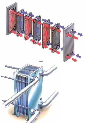
4.1.3. Plate heat exchanger (PHE) 44
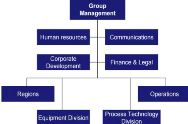
4.2. The Alfa Laval Organisation
46
4.2.1 Operation Development 47
4.2.2. Logistics 48
4.2.3. Supply Change 48
4.3. Enterprise Resource Planning System within Alfa Laval
49
4.4. Order Quantity
50
4.5. Reorder Point Principles
50
4.7. Service Level
52
4.8. Forecast Principles, SI & NI
54
4.9. Product costing according to MISAL
54
4.10. Purpose and benefit of product costing
55
4.11. Factory Cost according to MISAL
55
4.12. Activity Based Value Added Within Logistics
58
4.13. Theoretical Inventory Value
60
4.14. Classification of spare parts at Alfa Laval according to
Re-classification guide
60
4.14.1. Different reasons to change the standard classification 62
4.15. ABC classification of Stocked Items
63
4.16. Product Life Cycle
63
4.17. Obsolescence
63
4.18. Aspects on the spare part logistics from the sale segment
65
4.18.1. The long replenishment time on SI 65
4.18.2. The present SI-limit leads to different service levels 65 4.18.3. Production and spare parts are not synchronized 66
4.18.4. Competitive pirates in the market 66
4.18.5. One Four Eight 66
4.18.6. New type of classes 66
4.18.7. Clear the forecasts from abnormal values 67
4.18.8. Differentiated GO mark up 67
4.18.9. After sales service 67
4.19. Benchmarking toward other companies
67
4.19.1. Answer summary 70
5.
Analysis
78
5.1. Benchmarking of other companies
78
5.2. Overhaul of the present classification system
81
5.2.1. Different Inventory Classification Methods 84 5.2.2. +/- using classification methods with several criterions 88 5.2.3. Other factors that affects the classification 89
5.2.4. Introduction of certain limitations 90
5.2.5. What will happen if we classify from the other way? 93
5.3. ABC Classification
93
5.3.1. ABC Classification methods 94
5.4. Handling cost for items within each class
96
5.5. Statistics during more then 12 months
97
5.5.1. Forecast error 97
5.5.2. Analysis of demand during four years 99
5.6. Lead Time Analyse
101
5.7. Other Ideas
102
5.7.1. One global DC for low frequent spare parts 102
5.7.2. More focus on service 102
5.7.3. Store gaskets in vacuum 102
5.8. Simplicity
103
6.
Conclusion 104
6.1. Overhaul of the present concept
104
6.1.1. Item Classification 104
6.1.2. Number of items in stock 105
6.2. Specific questions
106
References
109
Appendix 1. Questions and answers to the benchmarking i
1. Introduction
The introduction chapter first contains a short description of the background to the problem. It continues with purposes, problem discussion, directives and delimitations.
1.1. Background
Alfa Laval is a company that develops, produce and sell products for heat transferring, separation and fluid handling on a worldwide market. The after sales market represents 25 % of their revenues.
In the year of 2002 Alfa Laval introduced a new classification system for their spare part inventory. Before this, the spare part supply system had been built up by multiple small warehouses located at the sales companies all over the world with a few larger centralized ones to supply them. In 2002 the number of warehouses was cut down and the world was divided up to three main business areas supplied by a few larger distribution centres (DC). Before 2002 there was no clear system that decided what should be kept in stock or not. The new system are based on that the products are divided in three main classes: stocked items (SI), non stocked items (NI) and request items (RI). Which class the items are assigned to depends on how many order lines (picks) the item have had during the last year.
After a few years Åke Skarstam and Richard Persson at the department of Operations Development thought that it was time to make a evaluation and perhaps further develop the classification system and worked out a specification for a master thesis. In this specification they also included what effect changes of some of the inventory level parameters would have and how universities and other companies handle similar situations.
Based on this specification we started to write our master thesis in September 2005.
1.2. Objectives
The main purpose of this master thesis is to make an overhaul of the present classification concept at Alfa Laval’s DC’s for spare parts. Another purpose is to increase customer satisfaction and to reduce or keep cost.
1.3.
Problem discussion and directives
The main purpose of this master thesis is to make an overhaul of the present classification concept at Alfa Laval’s DC’s for spare parts. Another purpose is to increase customer satisfaction and to reduce or keep cost.
The aim of Alfa Laval’s DC’s is to supply the customers with a high level of service in a cost efficient way for both parties. There are an endless number of
different possible combinations of approaches to reach this goal. Alfa Laval has chosen a quite simple inventory classification to decide if an item should be kept in stock or not. But even in a simple variant there are many parameters that can be more or less complex to control and understand.
Alfa Laval’s specified goal for this project is to increase customer satisfaction and to reduce or keep cost. This goal should be achieved by analyzing five different questions.
• What will happen if Alfa Laval classify from the opposite way? E.g. 96 % of all picks will define items as SI, 97-99 % as NI and the rest as RI. • What is the handling cost for items within each class?
• What is the effect of looking at statistics for more than 12 months?
• A lead time analyse. An item maybe does not need to be classified as SI if the lead time is short enough.
• Can Alfa Laval use other companies, the authors and universities ideas and if so, what are the plus and minus compared with our setup?
To be able to reach the goals we have included a lot of different factors that are essential to understand how complex the managing of a DC can be. When working with this thesis many different ideas has reached the surface and they are not always direct answers to the questions in the specification even though they are somehow connected. Often they are solutions which effect some of the parameters that affect the classification or the whole inventory management.
As a further step forward we have added a question that we think are relevant in this thesis.
• How can different parameters of the ABC-classification affect the cost and service of the items that are kept in stock?
This question aroused as a natural step of curiosity of what the effect could be when implementing different ideas one step further.
1.4. Delimitations
This thesis has almost only described issues that concern the spare part DC’s of Alfa Laval. Some of the ideas and approaches of this thesis could perhaps be implemented on other parts of the supply chain, but this thesis just briefly takes them into account. The reason for this is that it would require a lot of more time
than the 20 weeks we have for completing this thesis to get us acquainted with such a complex issue.
The data that has been used for calculations regarding the classification are solely from Alfa Laval’s DC in Staffanstorp and therefore the results from our analyse may give different results for another DC.
This thesis does not make any final judgements of how much that should be kept in stock. The data which we have based our analyses on are far to insecure to make such a judgement. We have presented examples of how different levels can be decided and are letting the inventory management at Alfa Laval make their own evaluations.
We have not considered the effect the amount of stocked items has concerning the capacity of the DC. E.g. if doubling the number of items in stock it would most certainly not be enough room for them in the warehouse.
Finally we have made the assumption that the price of all items are constant, regardless of order quantity and if they are stocked or not.
2 Methodology
This chapter describes the methods that have been used when writing this thesis. The theory behind the chapter is mainly collected from different methodology literature.
2.1. Investigative
approaches
In the planning and carrying out of an investigation it is important to do several decisions regarding the purpose, extent, what sources to use, what data gathering methods to use and which data that is necessary. (Lundahl, Skärvad, 1999)
The approach aims to the basic technical design of an investigation and indicates the depth in it. There are three ground categories in the approach. The case study approach represents a profound study of individual cases. To compare a group of cases at the same point of time is called a cross section approach. It is also possible to use a time series approach, which binds the investigation to the time development of one or several different occurrences. The choice of approach is often related to the investigators main interest in the analyzing and interpretation work.
There are several different dimensions in an investigation approach, were the first one refers to the depth of the investigation. The other dimension indicates whether the investigation is quantitative or qualitative and finally the third dimension shows if the investigation should be based on primary or secondary data. (Lekvall, Wahlbin, 2001)
Our approach in this thesis has been to do several cross section approaches. Different setups and differences of data have then been compared with each other.
2.2.
Quantitative and qualitative methods
To use a quantitative method means that you are measuring something, e.g. size or length. This method concludes in numerical observations or lets itself being transformed into such. Experiments, observations, tests and question forms are some examples of this method. Often implementing quantitative examinations consists of three phases; the planning phase, the data collection phase and the analytic phase. The planning phase first step is to specify, with the help of a literature survey, the theories that are going to be investigated. When the specification is finished, a plan how to carry out the examination is made up. In the data collection phase one of the basic conditions to receive proper measurements is to strictly follow the made up plan. The analytic phase usually consists of one describing and one analytic step. The analyse helps to elucidate if the collected
empirical material supports the theories that was specified in the planning phase. (Lundahl, Skärvad, 1999)
In most cases quantitative methods describes a few variables among a big representative selection. (Darmer, Freytag, 1995)
In our thesis we have used a quantitative method. We have basically followed the method as it is described above.
A qualitative method distinguishes of that it does not use figures. The primary purpose is to describe, analyse and understand individuals or groups, not to concentrate on proving if the information has a general validity or not. A pure qualitative examination does not care how the world is, but how it is being experienced. There for its mainly suitable for examine people’s experiences of phenomenons like sickness, success, working organization or payroll systems. The examinations are based on what people have said, written, thought, done and the results of human decisions and acts. (Lundahl, Skärvad, 1999)
Just like in the quantitative method, the evaluation of the result is also important in a qualitative method. According to Knutsson (1998), the best way to do this is to work according to the criteria’s reliability, transmutability and confirmation. Qualitative methods investigate a large number of variables among a small number of respondents. (Darmer, Freytag, 1995)
To achieve a higher validity in the material of an examination, it is possible to use a combination of the two methods, a method triangulation. The combination has its downsides when a recurrence of the examination could be hard to achieve and a combination of methods is often more resource demanding. (Darmer, Freytag, 1995)
2.3.
The Gathering of Data and Information
Data that already exist is often referring to secondary data, as someone else has gathered earlier for a different purpose. Data that you collect by yourself is called primary data, as you gather it yourself for a specific purpose. As the secondary data already exists and is simple and cheap to use, you try to use this type of information source as much as possible. If that is insufficient you have to complete it with primary data. (Eriksson & Wiedershiem-Paul, 1997)
2.3.1. Primary
Data
These methods could be used separate or in combination and carried out at different rates of standardisation.
Interviews are methods of collecting data were an interviewer asks questions or raises a dialogue with the respondents. In every survey it is important to clarify what type of interview that will be carried out, how respondents should be identified and contacted, what interview technique that should be used and also how the interview material should be registered, compiled and analysed. It is also important to clarify the problem and purpose of the interview to the respondent in order to receive the desirable result. (Lundahl, Skärvad, 1997)
Observations imply that the investigator observes a course of events relevant to the investigation during a specific time. There are several types of observations that affect the observed object in different ways. The degree of participation by the observer can vary from very intensive interaction to non-existing interaction. If the observed objects are fully informed about the observation you talk about an open or undisguised observation. The opposite is a hidden or disguised observation. . (Eriksson & Wiedershiem-Paul, 1997)
Questionnaires are used to collect standardized information. Different respondents answer the same kind of questions, which can be formulated either with pre-made answers or with open possibilities to answer the question. The answers of a questionnaire are delivered in a written form. This makes it extra critical to formulate the right types of questions. You have to know exactly what types of answers you are searching for, since there is difficult to elucidate the answers afterwards. (Eriksson & Wiedershiem-Paul, 1997)
The primary data gathered in this thesis consist of interviews, questionnaires and observations performed mainly with co-workers at Alfa Laval. A benchmarking was carried out in the following way: A total number of 18 companies in the manufacturing industry were contacted by email with a request of participating in a benchmarking about spare part logistics. A question form with 23 questions were sent out and on which 11 of the companies answered. The questions were put together in cooperation with Richard Persson. The answers were gathered in an excel-file for easier comparison. All the participating companies received a copy of the benchmarking results when it was finished.
2.3.2. Secondary
Data
Secondary data refers to data and information that is already documented by another person or organization and not collected or compiled mainly for our own investigation. It could refer to books, items, websites, databases, annual reports and different types of records and notes. Like in all forms of data gathering it is important to secure that the secondary materials precision, validity, reliability and relevance, are in relationship with the purpose and problem approach of the investigation. (Lundahl, Skärvad, 1997)
2.4. Statistical
Credibility
To gain credibility, an investigation must measure what it is intended to. It must be free from randomised measurement faults and the statistical decline should be random.
2.4.1. Validity
The definition of validity defined by Eriksson & Wiedershiem-Paul (1997) is the ability of a measurement instrument to measure what it is intended to measure. There could be aspects to a subject that are not included in the measurement that perhaps needs to be included to give a trustworthy conclusion. E.g., if an intelligence test measure the ability to remember things, it has measured an important aspect on intelligence, but not all aspects.
It is appropriate to separate between two aspects of validity, internal- and external. Internal validity relates to the conformity between concept and the operational (measurable) definitions of these. Thus it is possible to investigate the internal validity without collecting empirical data.
There are three types of validity problems: (Lundahl, Skärvad, 1997).
• The measurement tool only includes a part of the definition. The tool measures to little.
• The measurement tool only includes a part of the definition and in addition something else.
• The measurement tool includes the whole definition and in addition something else. The tool measures too much.
External validity relates to the conformity between the measurable values you receive by using an operational definition and the reality. The external validity is independent of the internal validity and it is not possible to evaluate it without knowing how the empirical data has been collected and how it looks like.
2.4.2. Reliability
Validity is the most important demand on a measurement tool. If the tool does not measure what it refers to, it does not matter if the measurement itself is any good. To determine if the measurement is good it has to be reliable. With reliability you concern the absence of randomised measurement faults. An investigation with good reliability is characterized of a measurement, which is not affected by who is performing it or under what circumstances it occur. Methods to increase reliability often involves different types of standardisation procedures that aims at securing that the measurement is implemented as identical as possible each time.
2.5.
Source of errors
During the work process of a report there are many different potential sources of errors. These sources can have great impact of the quality of the report. If the source of errors is notified in the beginning of the work, actions can be taken to prevent errors from arising and give misleading results. Being aware of the source of errors and trying to prevent them implies a more correct and reliable result. (Lekvall & Wahlbin, 2001)
2.5.1. Objective
error
If the purpose of the thesis is incomplete or wrongly defined the thesis can, even if it fulfils its purpose, be useless. The result of the thesis may not be relevant to the problem. It is of importance that the purpose of the thesis is carefully worked through and correctly formulated to obtain a useful result to the problem. In some cases our thesis are discussing situations that were not mentioned directly in the given specification. To avoid any misunderstanding the purpose of this thesis has several times been discussed with the supervisor at Alfa Laval. Therefore the final formulated purpose of this thesis corresponds well to the underlying problem and the results will be relevant.
2.5.2. Direction and content error
This error depends on the problem specification and arises if the problem has not been specified minute enough or specified in the wrong way. The delimitations might be inappropriate and give the thesis an incorrect direction. If the specification of the problem is incorrect the thesis might not fulfil the purpose. To ensure that this error did not arise, the objective of the thesis has been formulated in consultation with the supervisors at Alfa Laval.
2.5.3. Frame of reference error
Errors can arise in the search for references. All theories about the problem and the subjects might not be found. In this case important theories and references might not be used and evaluated. The theories and models found about the problem and subjects can be misunderstood. The theories found might e.g. be meant for another situation than the classification of spare part inventory. To prevent these errors from arising several different references have been used. We also analysed the suitability of each specific theory.
2.5.4. Data
error
Different data has been used in the analyses. In these data several errors might be found. The data can be incorrect because of input errors as e.g. quantity, standard price and lead time. The data such as lead time can be out of date since the data in the enterprise systems only are updated now and then. The data used in the analysis might also be incomplete because of mistakes and misunderstandings during the transfer of data. The data might also be incomplete because some data such as lead
time are missing for some components. In our thesis we have found many of those problems described above. These will be further explained in chapter 5.2 together with the data analyse.
2.5.5. Interview and benchmarking error
There can be different errors in the written and oral interviews with personnel at Alfa Laval and at the participating companies in the benchmarking. The respondent might not be able, or want to give us the correct information. This kind of problems likely occurs in this thesis but can not be fully prevented. These errors can not be prevented but has to be considered when the outcome is analysed. The questions in the interviews and benchmarking might be formulated in an inappropriate way. Because of this the questions might be misunderstood and the wrong answers given. The answers from the respondent might also be misunderstood or wrongly interpretive by the interviewer. The answers from the respondents have been considered as reliable and have not always been validated.
2.5.6. Analysis
error
Errors in the thesis can occur that are related from data that has been incorrect processed or analysed. This can lead to that the wrong conclusions have been made. To avoid those errors the data and calculations has been independently checked by both authors.
2.5.7. Interpretation
error
From the analyses it is possible that the wrong conclusions could have been drawn. The error can be related to lack of competence when converting the results into theoretical conceptions. To avoid this error the conclusions drawn from the analyses have been discussed with the supervisors at Alfa Laval.
2.6.
Objectivity and confirmation
The personal reference frame of the investigator has an influence on the result of the examination. It is disputed among scientist if it is possible or even desirable to achieve objectivity in social scientific research. According to Knutsson (1998), qualitative investigation work, is the term confirmation often used instead of objectivity. That means if the investigators interpretations are logically consistent against the research material or not. In practical research situations it is however often a demand that the result should be purpose. According to Lundahl, Skärvad (1999), it is important to realize that the word objectivity could have different meanings for different persons and situations, e.g. impartial, separation between facts and evaluations, multifaceted, complete. The investigator should be aware of his choice of perspective and evaluations that controls among others the formulation of the problem, method and conclusion and thereby report this in his description of the investigation process.
In this thesis we have tried to build our knowledge from as many sources as possible to keep up our objectivity. We have read and heard many different opinions of how things should be done during our time at Alfa Laval but we have tried not to adapt them in our analyse without carefully consideration.
It is always hard to find an outside reviewer whose competence is sufficient in the problem sphere, but we hope that the group of opponents of this thesis will secure our objectivity and confirmation in a satisfying way.
3 Theory
The purpose of this chapter is to give the reader knowledge about theories within inventory management which are of importance to this report.
3.1. Forecasting
There are two main reasons why an inventory control system needs to order items before the customer demands them. First, customers often require delivery in less then the replenishment lead time. Second, sometimes orders have to be made in batches instead of unit for unit due to e.g. high ordering cost. Once the forecast is established it is used to establish; order triggers, order quantities and SS levels. Other uses of forecast are to determine excess, surplus and inactive stock levels. All of this means that we need to look ahead and forecast the future demand. But to estimate the demand is not enough. We also need to estimate how uncertain the forecast is. If the forecast is more uncertain, a larger SS is needed. The difference between the forecasted demand and the actual demand is the forecast error. This is another important factor to estimate and is usually represented by the standard deviation or the Mean Absolute Deviation (MAD).
A suitable forecast method for inventory control typically involves a relatively short time horizon. It is seldom necessary to look more then one year ahead. There are several types of forecast techniques but the most common approach is based on extrapolation of historical data. This means that the forecast is based on previous demand data. The forecasting techniques are grounded on different statistical methods for analysis of time series. These forecasts are easy to apply and update in a computerized inventory control system with thousands of items.
Forecasts could also be based on other factors. It is common that the demand for an item depends on the demand on another item, e.g. an item is used as a component within another item. In this case it is suitable to first forecast the demand for the final product. Next a Material Requirements Planning-system (MRP-system) is used to obtain the demand for dependent items within the final product.
Several other activities could be considered when forecasting demand. Different market activities such as sales campaigns, introductions of new products, competing products from different companies, are factors that affects the forecast. In these cases historical data are no longer representative. It is difficult to take such factors in account in a computerized inventory control system. Instead adjustments have to be made manually in case of such events. Another way of forecasting is by looking at other dependencies. E.g. a forecast for the demand of ice cream could be based on the weather forecast. To forecast the demand of a spare part used e.g. in a machine, it is reasonable to assume that the demand for the spare part increase as the machine gets older.
3.1.1. Demand
models
Extrapolation of historical data is the most common approach to forecast the demand. In practise this is very seldom done. With thousands of items to take into consideration the initial work does not to seem to be worth the effort. This means there is not enough historical data and instead a demand model is created intuitively. The general assumptions are very simple. (Axsäter, 1991)
Constant model
In this model the demand in different periods are represented by independent random deviations from an average. The average is assumed to be relatively stable over time compared to the random deviation.
(Axsäter, 1991) t t
a
x
=
+
ε
where tx
= demand in period ta = average demand per period (assumed to vary slowly),
t
ε
= independent random (stochastic) deviation with mean zeroTrend model
In this model the demand assumes to decrease or increase systematically. The model is extended by also considering a linear trend. (Axsäter, 1991)
t t
a
bt
x
=
+
+
ε
where
a = average demand in period 0
b = trend, that systematically decrease or increase per period (assumes to vary slowly)
Trend-seasonal model
Here a seasonal index
F
t is introduced that decide the demand in period t. E.g. ift
F
=1.2, this means that the expected demand in this period is 20% greater due to seasonal variations. If there are T periods in one year, we must require that for any T consecutive periods TF
T
k k t=
∑
=1 +. By setting b = 0 in this model we obtain a constant-seasonal model.
t t t
a
bt
F
x
=
(
+
)
+
ε
where tF
= seasonal index in period t (assumed to vary slowly)When forecasting it is important to understand that the independent deviation
ε
t cannot be taken in account. This means thatε
t always has to be zero to do an accurate forecast. Consequently, if the independent deviations are large it is impossible to avoid large forecast errors. (Axsäter, 1991)Moving average
The moving average demand method is based on the same principles as the constant method. Assume the same underlying demand structure. The independent deviation
ε
t cannot be predicted so all we need to estimate is the average demand a. If a were completely constant, the best estimate would be to take the average of all observations ofx
t. If we assume that a varies over time, the problem is solved by looking at the most recent values ofx
t. The moving average is calculated by taking the average over the N most recent values ofx
t. (Axsäter, 1991)N x x x x a xt, t ( t t−1 t−2 ... t−N+1)/ ∧ ∧ + + + + = = τ
Where
t
a
∧ = estimate of a after observing the demand in period t τ,
t
x
∧
= forecast for period > t after observing the demand in period t.
Exponential smoothing
The result of this method is similar to the moving average method, but in this method the demand levels from past periods are weighted and affect the forecast differently. We assume a constant demand model and we estimate the parameter a. To update the forecast in period t the previous forecast and the most recent demand
t
x
is used. t t t t a a x x τ = = −α
− +α
∧ ∧ ∧ 1 , (1 ) whereτ
>
t
andα
= smoothing constant (0<α
<1).The value of parameter
α
is adjusted to historical data to obtain the best suitability. The exponential smoothing method could also be extended to include both trends and seasonal variations. If the smoothing method includes trends we now have to estimate both the average demand a and the trend factor b just as in the trend model previously explained. If the method also includes seasonal variations the Winters trend-seasonal method, which is a generalisation of exponential smoothing with trend, could be used. In this case the seasonal indexF
t has to be estimated as well. (Axsäter, 1991)Correlated stochastic deviations
In the methods previously used the stochastic variations where assumed to be independent. This is a major simplification and it is easy to think of situations where this is not true. E.g. if there are only a few large customers we can sometime expect demand in consecutive periods to be correlated. If there is a high demand in one period it is reasonable to expect that the demand in the next periods will decrease. The opposite could also be true, if there is a high demand in one period this may lead to high demand in the following period. Forecasting techniques that can handle correlated stochastic demand variations and other more general demand processes has been developed by Box and Jenkins. (Axsäter, 1991)
3.1.2. Low-frequent items
The forecasting methods we have discussed so far can sometimes be inappropriate for low-frequent items. Assume e.g. that a demand normally arises twice a year but then concerns large quantities. If we use an exponential smoothing method the forecast will increase just after the demand occurs and then gradually decrease until next demand arises. This unwanted effect could be reduced by using a small smoothing constant, but then the forecast will react very slowly to demand changes.
A different and more attractive method is to only update the forecast in periods with positive demand. Two averages are then updated by exponential smoothing: the size of the positive demand and the time between to periods with positive demand. This gives a more stable forecast and also shows the demand structure in a better way. (Axsäter, 1991)
Another opinion is expressed by Sussams (1988). Many companies have a problem with excessive stock, which can be defined as stock which provides a considerable higher service level than what is desired. This problem is especially common for the slow-moving items. To forecast the demand for a very slow moving item is not an easy task. For fast moving products, the exponential smoothing method or
regression analysis is used. These two methods will not give a good result when handling slow moving products because there is too few data to base the forecast on. Also it is very hard, or impossible, to see a trend in the demand. A better method in this case is the moving average (see chapter 3.1.1). This method is not as sensitive if the sales rate doubles or halves, which give a stabilising affect on the stock level control.
One way to keep the inventory levels down is to have a centralized stockholding. Then the amount of stock to cover the service-level is much less than having stocks dispersed in regional depots. Another advantage with keeping stockholding centralized is that there is more data to base the forecasting on. This is especially useful in the controlling of slow moving items. (Sussams, 1988)
3.1.3. A comparison between moving average and
exponential smoothing method
The two most common methods to calculate a forecast today are the moving average method and the exponential smoothing method.
Stig-Arne Mattson (2004) has made a report where he makes a comparison between these two. The analyses and calculations have been made in Excel and are based on randomly generated periods of demand with and without influence of trends and season variability. The quality has been measured with MAD, systematic forecast deviation and degree of instability between periods.
There is a simple relation between the number of periods in the moving average and the α-value in exponential smoothing method if both methods have the same average age on the included demand data. This relation can be described as:
α = 2/(n+1)
n= number of periods
The number of periods in moving average corresponds to the α-values in table 3.1.
α-value Number of periods
0,05 39 0,1 19 0,2 9 0,3 6 0,4 4 0,5 3
With exponential smoothing, at a random demand without any trends or season variability’s, a significant better forecast quality is maintained measured with MAD while using a α-value about 0,05. Regarding the systematic forecast deviation, the quality of the forecast is equivalent for different α-values. Also considering the degree of instability a α-value around 0,05 shows better result than higher α-values.
In demand-cases with a trend and a moderate varying demands around this trend, α-values around 0,2-0,4 gives the best quality of the forecast. If the demand varies a lot around the trend, α-values around 0,05-0,1 delivers a better result. The systematic forecast deviation diminishes with higher α-values, while the instability in the forecast increases with a higher α-value. When having season variability’s in the demand, a very small α-value gives the best results.
When having a random demand without any trends or season variability’s, a significant better quality of forecast measured in MAD with a moving average is maintained when a number about 18 periods is used. The authors of this thesis have also had a conversation with Stig-Arne about this and the 18 periods was the maximum number of periods that was investigated during his report. Stig-Arne thought that larger number of periods would give an even better result.
When having a low and very variable demand, a common spare part situation, a exponential smoothing with an α-value of 0,05 always seems to be preferable instead of a moving average irrespective of the number of periods. Regarding the systematic forecast deviation, the quality is similar for different number periods. Also concerning the forecast stability index, the quality of the forecast becomes better when more periods are included in the calculations.
3.2. Manual
Forecasts
The forecasting methods we have discussed so far are all based on extrapolation of historical data. There are situations when these forecasting methods are not suitable. Sometimes we know that there is factors that affect future demand, but which have no affect on the previous demand. These types of factors are very difficult to take into consideration in a computerized forecasting system. Usually it is much simpler to let manual forecasts replace forecasts based on historical data in such situations. Examples of situations when manual forecasts could be considered includes the following: price changes, sales campaigns, conflicts that affects demand, new products without historical data and new competitive products on the market. (Axsäter, 1991)
3.3.
Forecast errors and forecast control
Measurements of forecast errors are fundamental for all forecast control. Continuous measuring of forecast errors should therefore be a natural part of all forecast system. The purpose is partly to identify individual stochastic errors and
also to identify systematically errors, i.e. that the forecast is systematically too high or too low. If the forecast is too low it might lead to stock outs and if it is too high it might lead to overproduction and increasing stock levels. The size off the forecast error also decides the size of the SS. (Mattson & Jonsson, 2003)
To determine the size of a SS it is not enough to know the mean of the future demand. You also need to know how uncertain the forecast is, e.g. how large are the forecast errors in general? In statistics the most common way of describing variations around the mean is trough the standard deviation:
2
)
(
X
m
E
−
=
σ
where X is the stochastic variable, m its mean and E refers to the expected value. Standard deviation is equal to the square root of the variance,
σ
2. In connection with forecast errors another definition is used. By old tradition the Mean Absolute Deviation (MAD) is estimated. MAD is the mean value of the absolute deviation from the mean.The reason why MAD was estimated instead of
σ
was originally because of the simplified calculations. However this is not a problem today but the MAD-value is still used in most forecasting systems.It is obvious that MAD and
σ
in most cases measures the same thing. If we assume that the forecast errors are normally distributed it is possible to show this simple relationship:MAD
MAD
1
.
25
2
/
≈
=
π
σ
This relationship is used in most forecasting systems, also in situations when the assumption that forecasts errors are normally distributed is not valid.
A low MAD-value is not itself a good enough measurement on high forecasting quality. A good forecasting method should also give small average forecast errors in the long run, i.e. the forecast should give a low value just as often as a high value compared with the real demand. If the forecast method works ideally the average forecast error should equal zero. (Axsäter, 1991)
3.4. Lead
time
The time that passes from that a customer places an order until the order is delivered to the customer is called the lead time. If the lead time is tolerable or not
m
X
E
is decided by the market and the characteristics of the product. (Aronsson, Ekdahl & Oskarsson, 2003)
3.5.
Make to Order vs. Make to stock
3.5.1. Strategic
logistics decision making
Logisticians must make strategic level decision in order to manage uncertainty, customer service and cost. Wanke & Zinn (2004) explores the relationship between three strategic level decisions and selected product, operational and demand variables.
• Make to order vs. make to stock. • Push vs. pull inventory deployment.
• Inventory centralization vs. decentralization.
Strategic decisions are a function of product, operational and demand related variables such as delivery time, obsolescence, variation of sales and inventory turnover. E.g. Dell Computer uses a make to order system and pulls demand through by only manufacturing and distributing computers in response to a customer order. In this way the company maintains a minimal level of inventory. On the other hand Hewlett-Packard, a competitor of Dell, elects to manufacture products to stock based on a forecast. In this study Wanke & Zinn brings up earlier studies and compares them with result of their own analysis. The results shows that their analysis support earlier theories, which will be presented her.
There are six variables with reported relationship with the make to order vs. make to stock decision. Process technologies are either continuous or discrete. Make to order are more frequent in discrete process industries than in continuous process industries. This is because they are more flexible from a manufacturing point of view. If the risk of obsolescence for a product is large, the propensity towards make to order increases. This is because the risk of holding inventory is high and firms manage it by only producing sold items.
The coefficient of variations of sales is analogous to obsolescence. The lead time ratio is the quotient of the delivery time over the supplied lead time, which means how much time that is available to manufacture a product once it is sold. The smaller the time available, the more likely products will be made to stock. The greater the perish ability of the final product; the more likely that products are made to order to avoid loss of inventory. The study suggests that managers should focus on delivery time and coefficient of variation of sales as indicators of the make to order vs. make to stock decision.
The push decision moves products on the basis planning or forecasting, while the pull decision moves products based on demand. Since lower inventory levels are
more likely to be achieved under pull rather then push decision, variables that affect the inventory risks and carrying costs may influence the pull decision.
Obsolescence and delivery time are linked to the pull decision, delivery time because firms may not need to forecast if delivery time is long.
Demand information visibility is the extent that actual demand information penetrates a supply change towards the initial supplier, also known as order penetration point. The idea is that companies rely on planning inventories in the absence of actual demand information.
A high cost of good sold equals a high amount of working capital required. This may lead to a pull decision because the expensive inventory is an incentive to react to demand rather than to plan and keep products in inventory.
Cost density, coefficient of variation of sales, inventory turnover and delivery time are variables that may affect inventory decentralization. The lower the cost density, the higher the pressure to keep transportation unit costs down. Freight consolidation, which spreads transport fixed costs, can be achieved with inventory decentralisation. Freight consolidation also impacts the time between two replenishments and because of this the inventory turnover falls. Short delivery times could also lead to inventory decentralization.
3.5.2. Simple and combined inventory policies,
production to stock or to order?
In an inventory model three strategies can be applied. Either you decide between production to stock (s.S.), production to order (direct delivery), or production partly to stock and partly to order. Popp refers to this as simple or combined inventory policies. His study shows that the policy of direct delivery will be applied instead of the (s, S) when the holding costs are very high in relation to the setup costs. Then it is advantageous to hold no stock at all and to order each time when a demand occurs. This is true under some simplified conditions that, e.g. lead time for replenishments of stocks equals zero. The two simple policies can be combined so that larger demand values with lower probabilities are subjected to the policy of direct delivery and the smaller demand values. The conclusion is that in practise the combinations of two policies often occur when extreme demand values exist. (Popp, 1965)
3.6. Reordering
systems
One of the questions to answer when managing inventories are: when is the right time to order? In the following text the most common strategies of reordering systems are described. From these strategies numerous of variants could be found
but this thesis only describes the main strategies. Some of the terms often used in this part are expressed by Axsäter (1991) as:
Inventory position = stock on hand + outstanding orders – backorders Inventory level = stock on hand – backorders
SS = SS, explained further in chapter 3.8.
3.6.1. (R,Q)-system
One of the most common reordering point systems (ROP-system) are the (R,Q)-system. It implies that an order of size Q is placed every time the inventory position reaches, or drops below, the reorder point level R. The system is often used with either a continuous or a periodic review approach. If the inventory position has reached far below the R-level it might be necessary to order a larger quantity then Q to raise the inventory level above R. The size of the order can then be multiplied with n to reach above R. This variant of an (R,Q)-system is called a (R,nQ)-system. The reorder point is expressed as:
x
x
R
=
ˆ
+ SSWhere
xˆ
x= Expected average demand during lead time. (Axsäter, 1991)If R is recalculated continuously when changes occur in demand or lead time, the system is called a floating reordering point system. Most common is to calculate R periodically e.g. one or a few times per year. (Mattson, 2004)
Figure 3.1. (R,Q) policy with continuous review continuous demand. (Axsäter ,1991)
3.6.2. (s,S)-system
The (s,S)-system is a form of a ROP-system where s and S is equivalent to a reordering point and to a pre-specified order-up-to level. When the inventory position level reaches, or falls below, the level s an order is placed for the quantity that is needed to reach the inventory position S. This quantity is thereby variable and not fixed. Similar to the (R,Q)-system, this system can be used with a continuous review approach or a periodic review approach. If a continuous review approach is used and the demand always is one item the (s,S)-system is equivalent to a (R,Q)-system.(Axsäter,1991)
Figure 3.2. (s,S) policy, periodic review. (Axsäter, 1991)
3.6.3. S-system
To use a periodic review approach and have a fixed order period but a variable order quantity is called using an S-system. When working with an S-system the inventory position is at each inspection replenished up to the order-up-to level S regardless of if the inventory position has reached the reorder level s or not. (Axsäter, 1991)
3.6.4. MRP-system
A material requirements planning system (MRP-system) differs from ROP-systems and considers that items demands can be dependent of one another. The technique is especially useful for items with occasional big demands. When an item is used to produce another item the dependency is called to be vertical. When an item instead is attached to another product, e.g. a remote control for a stereo, the dependency is called horizontal.
MRP-planning makes following assumptions:
• A production program for the end-product has to be updated continuously. The program has to include all the needs that can affect the present purchase planning of components and raw material. The time horizon should therefore reach over the total lead time from purchase to finished item.
• External needs for items that are not end-products e.g. spare parts.
• A structure register, that is specifying the connections between different items, is required.
• Statistics of stock on hand, outstanding orders and backorders has to be available.
• Lead time for all the items has to be known. (Axsäter, 1991)
3.7. Order
Quantities
The ordered quantity should cover the need that exists or expects to exist. An obvious way of deciding the right ordering quantity is therefore to let the order correspond to every single need, which means that a new order is created for every need and the order quantity correspond to the size of the need. For a lot of reasons it is not always suitable or possible to manufacture or procure the quantity that is needed at every single occasion. The reasons could be of both technical and economical natures. Needs from several sources has to be collected to larger order quantities. (Mattson & Jonsson, 2003)
When we have decided to use larger order quantities, next question to answer will be how large order quantity (Q) should be ordered? In this chapter we describe the most relevant methods for deciding the right order quantity.
3.7.1. Fixed Order Quantity (FOQ)
This method is based on a fixed order quantity that is decided intuitive or from previous judgements. These judgments could be based on estimated annual consumption, price, order cost and obsolescence. The order quantity is judged at every re-order point and varies from time to time. The conditions under which the FOQ technique may be considered includes (Bernard, 1999), (Mattson & Jonsson, 2003):
• Quantity may be fixed at a standard container, unit load or shipping load. • Limited shelf space.
• There may be a requirement to purchase a supplier’s standard production lot size.
• The company may elect to take advantage of a particular supplier price break.
3.7.2. Period Order Quantity (POQ)
A period order quantity covers the total demand for a specified number of periods. The time period remains constant while the order quantity varies since demand varies from period to period. This system is the opposite of the fixed order quantity system. Periods may be selected as shifts, days, weeks, etc. All demand during a period are added and ordered together. If there is no demand there is no order. A situation where periodic ordering is used could be when deliveries require a time period equal to the delivery or pickup cycle, e.g. a shipment that arrives in port once a month. (Bernard, 1999)
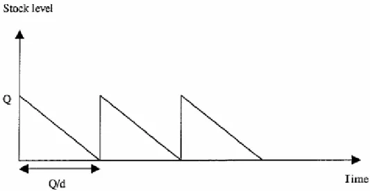
3.7.3. Economic Order Quantity (EOQ)
The most commonly used method to decide the right order quantity by mathematical calculations is the economic order quantity formula. It is also known as the square root formula or the Wilson formula after one of its creators. The calculations are based on a minimization of the total cost, which is a combination of the inventory holding cost and the ordering cost. The model is based on the following assumptions:
(Mattson & Jonsson, 2003)
• The demand per time unit (d) is constant and known.
• The lead time for inventory replenishment is constant and known.
• The ordering cost (A) or the setup cost is known and independent of the order quantity.
• The inventory holding cost (h) per unit and time unit is constant, known and independent of order quantity.
• The order quantity (Q) does not need to be an integer.
• The replenishment of inventory is instantaneous, i.e. the whole order quantity is delivered at the same time.
• No shortages are allowed.
• The price and cost for each unit is constant, known and independent of order quantity and place of purchase/manufacturing, i.e. no discount are allowed.
Since no SS is needed in this model the inventory level will vary over time as in Figure 3.3.
Figure 3.3. Development of inventory level over time. (Axsäter, 1991)
The total cost per time unit equals the holding cost and ordering cost. We Obtain. (Axsäter, 1991) Total Cost
A
Q
d
h
Q
C
=
+
2
)
(
The cost function can be minimized with respect to Q. The first order condition gives us
0
2
−
2=
=
A
Q
d
h
dQ
dC
Solving for Q we obtain the economic order quantity:
h Ad Q∗ = 2
If we insert
Q
∗ in the cost function we get:Adh Adh Adh C 2 2 2 + = = ∗
This equations state that the economic order quantity is the point where the holding cost equals the ordering cost. This relation is illustrated in fig. 3.4.
Figure 3.4. Connections between order quantity and ordering cost. (Mattson & Jonsson ,2003)
As figure 3.4 shows, the total cost curve is very flat near its optimum. This means that total cost would not changes much if the order quantity differs from the optimal value. Thereby the economic order quantity is relatively insensitive for errors in the other parameters as well, e.g. demand or holding cost.
It exist a large amount of variations of the economic order quantity formula. Most of these variants are characterized by that some of the assumptions in the original formula has been modified or eliminated. This makes it possible to develop models that take other factors in considerations. E.g. finite production rate, quantity discounts and shortages. These variants will not be covered in this thesis.
(Mattson & Jonsson, 2003), (Axsäter, 1991)
3.7.4. Lot-for-Lot
(L4L)
This method is the simplest and one of the most commonly used ways to determine the order quantity. The method means that the order quantity equals a unique demand. This method results in lower holding costs, since there is no inventory, but also higher ordering costs.
The L4L method may be considered in the following situations:
• Materials are purchased for a specific customer order, which cannot be applied to other orders.
• Parts may regularly undergo engineering revision changes over time. Using the L4L ensures that only sufficient quantities of each revision are ordered. • The ability to bypass MRP and generate orders directly from the bill of
material explosion process.
• When a part is being phased-out. This limits the risk of generating excess, surplus, inactive and obsolete inventory. (Bernard, 1999)
3.7.5. The Wagner-Whitin algorithm and the
Silver-Meal heuristic
The EOQ model assumes constant demand. If demand varies over time there are different methods for calculating the right order quantity. The object is, like before to choose the order quantity that minimizes the sum of the ordering and the handling cost. The difference is that we can no longer expect the order quantity to be constant. These problems are solved by using Dynamic Programming. The total costs are calculated each period. For each period there are two alternatives, either to order the demand needed for the current or future periods, or already having it in stock from preceding periods. An optimal method for solving this problem is the Wagner-Whitin algorithm. Since the method comprises of extensive calculation it is seldom used in practice. Instead a simplified calculation that gives a solution close to optimum is used: The Silver- Meal heuristic. (Axsäter, 1991)
3.8. Safety
Stock
(SS)
When a suitable order quantity and reordering point is chosen it is time to find a proper SS level. The demand is often looked upon as normally distributed and deterministic, even though the actual demand is known to be stochastic. There is a risk that a stock out situation will occur during lead time if the deterministic demand becomes below the actual demand. On the other hand there is a risk of an ascending deterministic demand inventory if the actual demand is lower. The SS (SS) is used to cover those random variability’s for the demand during lead time. How big the SS should be depends on how big the insecurity is in the deciding of the demand and how the service level(chapter 3.9) is set. There is also a possibility to base the SS on a shortage model instead of service level, but it is not the most commonly used method. (Axsäter, 1991)
3.9. Service
level
The concept service level is an expression for ability to deliver to customer. (Mattsson, 1997)
There are a number of different pieces in the puzzle to make a customer satisfied. To make the whole service package work it is important to be aware of all of these pieces. Aronsson, Ekdahl & Oskarsson define seven pieces that could have different importance depending on the business-situation.
• Lead time- The time from reception of the order to delivery to the customer. This is often especially important when handling spare parts. • Delivery reliability – To be able to deliver at the right time. The
• Delivery dependability – To be able to deliver the product in the right amount with the right quality.
• Information – When lead time is becoming more and more important it helps to exchange information to secure an ideal delivery.
• Customization – To be able to carry out the customer’s particular demands. Perhaps have the product delivered in a specific way or with a faster transportation.
• Flexibility - Be able to adjust to suddenly changed conditions.
• Order fill ratio – The part of the orders, or order lines, which can be delivered direct from stock.
In addition to the enumerated factors above, Aronson, Ekdahl and Oskarsson (2003) present the cycle service level and the fill rate as factors that also are related the service level. These are connected to the stock outs in a company and together with the other seven they are evaluated by the customer. To make the customer satisfied it is important to keep a satisfactory level on all the factors. What satisfactory levels are, is up to the customer to define, though it is also equally important to estimate them from the companies point of view.
3.9.1. Different
measures
Most of the service level factors are quite uncomplicated to monitor and evaluate, but the information, customization and flexibility factors are different. These three are so called soft factors and are rather hard to measure in numbers. Nevertheless, they are not of less significance than the other factors that affect the service level. (Aronsson, Ekdahl & Oskarsson, 2003)
The joint factor for the service level definitions are that they measure how well the company are satisfying different demands from the customer. For each definition it is possible to define a number of different targets. Each target must have a timeframe and it is easier to reach the wanted level with a longer time period. The timeframe must be carefully decided to suite the different situations. Using different timeframes can generate valuable information for the company about how things work in altered time perspectives. The company must set desirable target levels for the different factors to achieve and uphold. The target levels should be set so that they are attractive for new customers and satisfying for the old customers. (Hadley, 2004)