2013:28 Brine intrusion by upconing for a high-level nuclear waste repository at Forsmark. Scoping calculations

(1)

Research

Brine intrusion by upconing for a

high-level nuclear waste repository

at Forsmark

Scoping calculations

2013:28

Authors: Georg A. Lindgren Clifford Voss Joel Geier

(2)

(3)

SSM perspective

Background

SSM currently reviews a license application for a spent nuclear fuel re-pository that is proposed to be located at Forsmark, Sweden. The repo-sitory is to be situated at 500 m depth in the rock and copper canisters are deposited in holes excavated from the tunnel system. To protect the canisters they are surrounded by a bentonite clay buffer, which is to swell when getting in contact with water. The swelling properties are dependent on the salt content of the water and excessively high salt contents may inhibit the swelling. Thus it is important to ensure that the bentonite is not subjected to water with too high salt contents. The salt content of the groundwater increases with depth and is expected to reach levels that may affect buffer performance at large depths. When excavating the repository very high hydraulic gradients are established and water and salt movement from the depth to the repository, so-called ‘upconing’, could possibly occur.

Objectives

The objective of this study is to evaluate the possibility of salt-water mig-ration to the repository. This objective is motivated by the adverse im-pacts of water with too high salinity entering the repository and by the uncertainty of the relevant hydraulic and hydrogeochemical conditions at the Forsmark site at great depths. To analyse density dependent flow and salt transport at the Forsmark site the USGS’ SUTRA code is used. This study proceeds by finding critical model cases for which upconing does or does not occur, while assessing whether the parameterizations of these cases are realistic for the Forsmark site. In addition, the fall of the upconed salt mound (i.e. downconing) following closure of the repo-sitory is also evaluated. In particular the objectives are (1) to determine the factors that control saltwater upconing in a hydrogeological setting representative of Forsmark; (2) to relate these factors to the plausible conditions prevailing at the repository site; (3) to investigate whether the proposed repository is likely to generate saltwater upconing, given the range of uncertainty in hydrogeologic structure and parameter values; and (4) to evaluate the timing of upconing (salinization) and the timing of downconing (freshening) following repository closure for cases where upconing occurs.

Results

The results of this simulation analysis show that upconing behavior is strongly affected by the ratio of permeability to porosity in any zone in which upconing might occur. Within the full range of parameters that are likely to occur at the Forsmark site, the model yields either no signi-ficant upconing at all during the operational period of the repository or intrusion of brine-type waters after only one to a few decades.

(4)

Need for further research

A relatively simple conceptual model like the one used in this study is helpful in defining the modes of upconing behavior that are possible, and in defining the factors controlling this process. More elaborate structural models could be used to check more carefully which of the range of conditions that are here found to be plausible for the Forsmark site are most applicable.

Project information

Contact person SSM: Georg Lindgren Reference: SSM 2010/2105

(5)

2013:28

Authors: Georg A. Lindgren1)_{, Clifford Voss}2)_{and Joel Geier}3)

1)_{Swedish Radiation Safety Authority,}2)_{US Geological Survey,} 3)_{Clearwater Hardrock Consulting}

Brine intrusion by upconing for a

high-level nuclear waste repository

at Forsmark

(6)

This report concerns a study which has been conducted for the Swedish Radiation Safety Authority, SSM. The conclusions and view-points presented in the report are those of the author/authors and do not necessarily coincide with those of the SSM.

(7)

1. Introduction

BRINE INTRUSION AND REPOSITORY SAFETY - In Sweden’s

pro-posed high-level repository located at Forsmark, Sweden (Figure 1), spent nuclear fuel is planned to be encapsulated in sealed cylindrical copper canis-ters (about 1 m diameter and 5 m high) and disposed of in cylindrical holes (about 1.80 m diameter and 7 m deep) at around 500 m below ground level in fractured crystalline rock. The repository is intended to contain and isolate the nuclear waste for over 100,000 years. The holes are to be excavated in the floors of a tunnel system in the rock (deposition tunnels 4.8 m high and 4.2 m wide) that extends from the ground surface to this depth (SKB, 2011). Due to very low groundwater flow within the repository host rock, the tunnel and deposition holes will remain relatively dry during excavation and canis-ter emplacement (Svensson and Follin, 2010). The caniscanis-ters are smaller than the deposition holes and within each deposition hole, the canister will be fully surrounded on all sides by a so-called ‘buffer’ composed of bentonite clay that swells when it absorbs water. When the canisters have been em-placed and surrounded by relatively dry but pure bentonite, the tunnel seg-ments are closed off by backfilling with swelling Friedland clay. Then the backfilled tunnel and deposition holes slowly begin to resaturate with groundwater that flows in from the host rock. During resaturation, the swell-ing bentonite should fill all voids in the deposition holes between the canis-ter and host rock, leading to a very dense barrier that allows only diffusive transport of solutes through the clay, protecting the canisters from corrodants within the groundwater and surrounding rock. This buffer also slows poten-tial outward transport of leaking radionuclides, should any canister not be thoroughly sealed or somehow compromised at a later time.

However, salty water exists in the host rock and bentonite swelling is ad-versely impacted by the salt content of the water it absorbs (e.g. see

Karnland et al., 2005); high salt content inhibits swelling. Thus, should salty groundwater enter some deposition holes and the tunnel during excavation and/or resaturation following repository closure, the resulting barrier may not meet the design requirements. Should the buffer not fully expand to fill the excavation voids as intended, its isolation function as one of the primary barriers within the repository’s multi-barrier waste isolation system would be disturbed, adversely affecting the repository’s ability to isolate nuclear waste, thereby decreasing safety margins. High salt content of the water flowing into the tunnel during excavation and emplacement may also be of concern for technical installations needed for the operation of the repository.

BRINE EXISTENCE AND MIGRATION AT FORSMARK - The salt

content of groundwater in the fractured rock at the Forsmark site increases with depth (SKB, 2008). Based on extrapolating data from Forsmark and similar sites to greater depths, groundwater consisting of brine likely exists

(9)

at shallow-enough depths (around or less than 2000 m) such that upward migration of brine to a repository at 500 m depth could occur via driving forces described in the following.

When tunnels are excavated and exposed to the atmosphere, the water pres-sure at tunnel depth drops drastically from hydrostatic prespres-sure of 50 atmos-pheres (5000 kPa) to atmospheric pressure (1 atmosphere or 100 kPa). This 50-fold decrease in pressure leads to a large hydraulic gradient in the groundwater around the excavation and thereby to an inflow of groundwater to the repository from all sides and an escape of air through the tunnel venti-lation system. Relatively fresh groundwater (with low total dissolved solids content) will initially enter the repository through transmissive fractures from above and freshwater inflow will continue as long as there is a surface source of water, such as rainfall recharge, snowmelt or fresh surface-water bodies. Groundwater with low to intermediate ambient salinity may flow into the repository from the sides through transmissive fractures connected laterally to the repository. However, the focus of concern in this study is the potential for upward flow in a flow field that results from such a large pres-sure disturbance in a fluid distribution that generally exhibits increasing salt content and fluid density with greater depth. After repository excavation, the driving force for upward flow due to the low repository pressure is in oppo-sition to the downward force due to buoyancy, in which denser salty water tends to sink. If the upward pressure force exceeds the downward buoyancy force, an upflow of relatively dense water with high salt content from depth may occur and may reach the repository. Such so-called saltwater upconing is a ubiquitous phenomenon in wells producing groundwater from coastal aquifers subject to seawater intrusion, having been widely-studied for pur-poses of water quality management, both experimentally and via numerical modelling (e.g. Reilly and Goodman, 1987; Prieto et al., 2006; Werner et al., 2009). Following repository closure, when the normal near-hydrostatic pres-sures are restored, ending the strong upward force, so-called downconing may occur, as any saltwater that has risen above the depth at which it is sta-ble moves downward via buoyancy forces, which persist until the saltwater has reached its stable depth.

For the Forsmark site, Svensson and Follin (2010) calculated the influence of repository construction on groundwater flow and migration of saltwater using a 3-D finite volume continuum porous media model. The data underly-ing the model was taken from a detailed three-dimensional site-descriptive model of the Forsmark site (SKB, 2008). The transmissivity and porosity data used were based on a hydrogeological discrete-fracture network model of the area. The results for this particular description of the site indicated that upconing of water with high salinity during repository excavation would not occur. An earlier study by Svensson (2006) predicted small impacts of an open repository on the migration of saltwater, although uncertainties were

(10)

not elaborated. Despite these reported results, SKB (Swedish Nuclear Fuel and Waste Management Co), the organisation in Sweden tasked with devel-oping Sweden’s high-level nuclear waste repository, concluded at the end of the initial site investigation stage that one of the main hydrogeological un-certainties was the possibility for upconing of deep saline groundwater in steeply dipping rock deformation zones with relatively high transmissivity (SKB, 2008).

THIS STUDY - Motivated by the importance of the potentially adverse

impacts of saltwater entering the repository and by the uncertainty of previ-ous studies for the Forsmark site, this study evaluates the possibility of salt-water migration to the repository. To ensure that the excavation and em-placement phase of the repository can be managed in a safe manner, to en-sure that the state of the repository prior to cloen-sure is well defined and well understood, and to ensure that the long-term safety of the repository will occur within planned margins (with particular regard to the performance of the bentonite buffer), it is important to develop understanding of potential inflow of saltwater into the tunnels in a more general manner than has been done previously, by considering a full range of possible structural configura-tions and hydrogeologic parameter values at the Forsmark site.

This study proceeds by finding critical model cases for which upconing does or does not occur, while assessing whether the parameterizations of these cases are realistic for the Forsmark site. In addition, the fall of the upconed salt mound (i.e. downconing) following closure of the repository is also evaluated. To accomplish generality, this study focuses on modeling two-dimensional (2-D) groundwater-flow and solute transport within a typical sub-vertical deformation zone that is parameterized based on site-specific data. The conceptual models are implemented in the U.S. Geological Sur-vey’s SUTRA finite-element code (Voss and Provost, 2002) that numerically calculates variable-density groundwater flow and advective-dispersive salt transport.

This groundwater simulation analysis thus has the following general objec-tives.

1- Determine the factors that control saltwater upconing in a hydrogeo-logic setting representative of Forsmark.

2- Relate these factors to the plausible conditions prevailing at the re-pository site.

3- Investigate whether the proposed repository is likely to generate saltwater upconing, given the range of uncertainty in hydrogeologic structure and parameter values.

(11)

4- For cases where upconing occurs, evaluate the timing of upconing (salinization) and the timing of downconing (freshening) following repository closure.

These results may then be employed to assess the possibility that saltwater will enter a Forsmark repository, and if so, for how long it may remain with-in the repository, so that possible adverse impacts on bentonite buffer swell-ing can be subsequently evaluated.

(12)

2. Methods

CONCEPTUAL APPROACH - Groundwater flow and salt transport in the

fractured rock surrounding the planned Forsmark repository occurs primarily through a sparse set of structures consisting of intersecting vertical or sub-vertical and gently dipping fracture zones (deformation zones). Although some flow may pass laterally from one structure to another through the net-work of fractures in the rock domain, the primary impact of depressurization of repository tunnels is in the vertical direction, potentially resulting in up-coning of saline water and downflow of shallow fresh water. Thus, vertical or sub-vertical zones that connect deep brine with the repository and the ground surface are the most important conduits for the process under consid-eration.

For the current analysis, the system is evaluated by simulating 2-D flow through sub-vertical deformation zones that transect the repository domain, defined as the area within the repository outline (Figure 1). Based on the repository outline proposed by SKB (SKB, 2009) the deformation Zone ENE0061 is chosen as a reference point for conceptualizing the problem (Figure 1) and the geometry of this zone is roughly used to define the geom-etry of the conceptual model. From this reference point, the analysis then explores a variety of cases based on data not solely related to the zone. In this way, a variety of deformation zones with differing hydrogeologic prop-erties and differing external forcings that transect the repository domain are evaluated. Furthermore, the modeled cases specifically represent properties of Zone ENE0061 and Zone NNE0725 (for brevity, referred to herein as Zone 61 and Zone 725); these cases also cover a plausible range of property values for zones intersecting the Forsmark repository domain.

The model is conceptualized as a 2-D representation of a generic sub-vertical (i.e. nearly vertical) rock deformation zone that stretches from the ground surface down to the chosen bottom boundary of the model. The lateral length of the zone is taken from Figure 1 to be 2100m corresponding to the length of Zone 61. At its lateral ends, Zone 61 is intersected by other sub-vertical deformation zones. There are also several other sub-vertical zones intersect-ing Zone 61 (Figure 1). The deformation zone is also intersected by a large number of smaller fractures. It is assumed that the flow in the zone is sub-stantially larger than the flow through the smaller fractures and these smaller fractures are therefore not explicitly represented in the model. This is in ac-cordance with the conceptualization of the system used by SKB (SKB, 2008). SKB distinguishes between a hydraulic conductor domain, which ordinarily corresponds to a major deformation zone, and a hydraulic rock domain, which is made up of a discrete fracture network in the surrounding rock.

(13)

Figure 1. Map of Sweden indicating the location of Forsmark (above) and the layout of main and transport tunnels of the proposed repository at 470m depth at Forsmark (below). Zones ENE0061 and NNE0725 are indicated by arrows (modified from SKB, 2009, Fig 4-16). The regularly-spaced deposition tunnels with the waste canisters and bentonite buffer extend nearly perpendicularly to the main tunnels, with the ap-pearance of teeth on a comb that nearly fill the repository domain outline that is de-lineated by the surrounding transport/main tunnels (see SKB, 2009, Fig 4-13 for details).

ENE0061

(14)

NUMERICAL MODEL - The numerical calculations of the various cases

investigated in this study are carried out using the U.S. Geological Survey‘s SUTRA code (Voss and Provost, 2002). The SUTRA code can simulate fluid movement and the transport of salt in a subsurface environment. The code employs a 2-D or 3-D (three-dimensional) element and finite-difference method to calculate numerical solutions to variable-density flow and solute transport problems.

(15)

3. Data

The full set of parameter values derived from SKB’s site investigation data are used as a starting point for building the generalized models. Because the data and the assumptions used to derive the values are subject to some uncer-tainty, a Base Case model is set up to serve as a starting point for checking how changes in the assumptions and parameterization influence the up-coning results. The ranges of the input parameters used in the model span the ranges observed at the Forsmark site.

SALINITY - The salinity of the water at the Forsmark site has been

investi-gated by SKB (SKB, 2008) to a depth of almost 1000m. Figure 2 shows a compilation of salinity data (total dissolved solids) and least square linear depth-salinity fits for borehole data from Forsmark and Laxemar, Sweden, and Olkiluoto, Finland. Smellie et al. (2008) infer that drilling deeper than the available boreholes at the Swedish site investigation sites would intercept brines. In view of this assessment, SKB’s salinity model results for Forsmark are here extrapolated to a depth where the salinity reaches brine levels (100g/L). This is found to occur at about 2100m depth, motivating use of a groundwater model domain reaching down to that depth. The extrapolation gives higher salinities at depths than the extrapolation of the KFM07a and KFM09a borehole salinity data, but lower values than the extrapolation of data from Laxemar, Sweden (deepest borehole KLX02) and Olkiluoto, Fin-land.

(16)

Figure 2: a) Compilation of selected salinity data (total dissolved solids) from For-smark, Laxemar, and Olkiluoto together with linear extrapolations of the data to greater depths using a linear least squares fit. For Forsmark the two boreholes with the highest salinity values are shown (KFM07a, green triangles, Berg et al. (2005) p. 33; and KFM09a, black diamonds, Nilsson (2006) p.33). SKB’s model for salinity against depth for the so called Forsmark footwall* below 500 m depth is extrapolated to larger depths than shown in their Figure (magenta line, SKB (2008), Figure 8-46 p. 276). Laxemar data show the deepest borehole KLX02 below 1000m (red open cir-cles, Laaksoharju et al. (1999) p. 30; contributions from Mg, HCO3, Si, Li, Sr, and K are neglected). Olikiluoto data are from 2008 (blue filled circles, Pitkänen et al., 2009). Higher salinities than given in the 2008 dataset have been reported from Olki-luoto with a maximum of 84g/L (Pitkänen et al., 2009 p. 83 ). *Note: The footwall is defined as the body of rock that lies beneath the set of gently dipping deformation zones in the south of the investigated area.

b) Map showing location of salinity data measurements at sites within Sweden (left on the map) and Finland (right), all located along the coast of the Baltic Sea and Gulf of Bothnia. 0 20 000 40 000 60 000 80 000 100 000 120 000 -1800 -1600 -1400 -1200 -1000 -800 -600 -400 -200 0 Salinity (mg/l) D e p th ( m )

Olkiluoto (data below -350m included in fit)

KFM09a

KFM07a (data below -500m included in fit)

Extrapolation of deep end of salinity modelled by SKB

for Forsmark footwall

KLX02 (data below -1000m included in fit)

N

Olkiluoto Laxemar Forsmark 300 km a) b)

(17)

PERMEABILITY - The transmissivity range of the modeled generic

de-formation zone is based on data from SKB’s site investigation. Zones that connect the repository at about 500 m depth with possible brine at greater depths are the ones that might conduct brine to the repository and are thus the focus of this analysis. Two zones, one with relatively low transmissivity (Zone 61) and one with relatively high transmissivity (Zone 725) are chosen as reference parameterizations for the model (Table 1). Both zones intersect the repository tunnels and thus may contribute water inflow to the reposito-ry.

The transmissivity of Zone 61 is close to the lower limit of what can be measured and can thus be argued to be a lower limit for transmissivity. There are many zones with transmissivity below the measurement limit (Fol-lin et al., 2007, e.g. Table 9-1), but these will host less saltwater upconing than zones with higher transmissivity, so can be neglected in this analysis. Considering a high transmissivity limit, Zone 725 is the most transmissive that crosses the repository domain (based on information in Follin et al, 2007, and Stephens, 2007). There is one zone with higher measured trans-missivity at relevant depth outside the repository domain, but this will not impact upconing in the repository domain. There are no transmissivity data for depths greater than 900 m and because connections to brines at depths of as much as 2100 m must be considered, the transmissivity at these depths must be extrapolated from shallower data.

There are many gently dipping zones with transmissivity greater than Zone 725 (Follin et al., 2007, max 1.2x10-3 m2/s at 130 m depth, i.e. almost 4 or-ders of magnitude greater than Zone 725), but these lie above and partly outside the repository domain. There is one measured zone at about 430 m with transmissivity of 1.2x-10-6 m2/s, half an order of magnitude greater than Zone 725 and also at a relevant depth. However this zone lies at the border of the repository domain and will not directly impact the repository. There are also structures at depths less than 300 m that are more transmissive (maximum about 2 orders of magnitude greater than Zone 725 at 200 m depth). However (as will be clear from the results presented later in this analysis), the transmissivity of structures below the repository, not above, exert the greatest control on upconing behaviour, so the shallow high trans-missivity structures are not as important in the current analysis.

Because variable-density flow is simulated, the SUTRA model requires permeability values and so the transmissivities derived from SKB’s meas-urements need to be expressed as permeabilities. To accomplish this, hy-draulic conductivity values are first calculated from the transmissivities, requiring definition of zone thicknesses, which are based on data from the boreholes that intersect the zones. Zone 61 is intersected by borehole KFM01d and KFM06a and Zone 725 is intersected by borehole KFM 06a (SKB, 2007). In Table 1, all the data required for calculating the

(18)

permeabil-ity of the zones from available measurements are given, together with the respective references. For all modelled cases except the spatial trend and heterogeneity cases the permeability is assumed to be constant throughout the model domain. When there are measurements of the transmissivity from several measurement sections in the borehole interval in which the defor-mation zone is located, the transmissivity values are summed to get the total transmissivity of the zone. The hydraulic conductivity is then calculated by dividing the transmissivity by the zone thickness. For Zone 61, the geometric mean of the conductivity values from the injection test measurements in the two borehole intersections is used to calculate the effective conductivity of the zone. This is based on the fact that, assuming 2-D steady flow in an un-bounded isotropic lognormal conductivity field, the effective conductivity can be calculated by taking the geometric mean of the measured values (e.g. Rubin, 2003). The permeability k is then obtained from the conductivity using

ms with K being the hydraulic conductivity (m/s),

µ the dynamic viscosity, ρ the density of water and g the gravitational accel-eration. For Zone 61, this yields a permeability of 6.7x10-18 m2 and for Zone 725, 1.8x10-15 m2 (using the geometric mean of the measurements with the two methods). (The available ‘difference flow meter’ measurements are not used for Zone 61, since they are close to the measurement threshold (Hjerne et al., 2005, Väisäsvaara et al., 2006) and the injection test results are con-sidered more trustworthy).

POROSITY - To calculate transport of dissolved salt, the effective porosity

values of the deformation zones are required. For all modelled cases except for some spatial trend cases the porosity is assumed to be constant through-out the model domain. The effective porosity value 9x10-4 is used for repre-senting Zone 61. This number is obtained by dividing the sum of apertures in the interval (calculated by summing the apertures described in Pettersson et al. (2005)) by the length of the borehole interval. Both 0.028 m/30 m and 0.02 m/20 m yield approximately a porosity of 9x10-4. For Zone 725, similar reasoning yields a porosity of (0.05 m)/(35 m) = 1.4x10-3. This calculation assumes that all fractures with an aperture in the interval that the zone inter-sects are parallel to the zone and participate in carrying active groundwater flow. Since many of the indicated apertures are close to the resolution of the method, these were assigned 0.5 mm (Pettersson et al., 2005 and 2006). The actual porosity of the zone at the borehole intersection may thus differ from these calculated estimates. This and the very likely spatial variability of the porosity within the zone make a sensitivity analysis necessary for a range of porosity values.

(19)

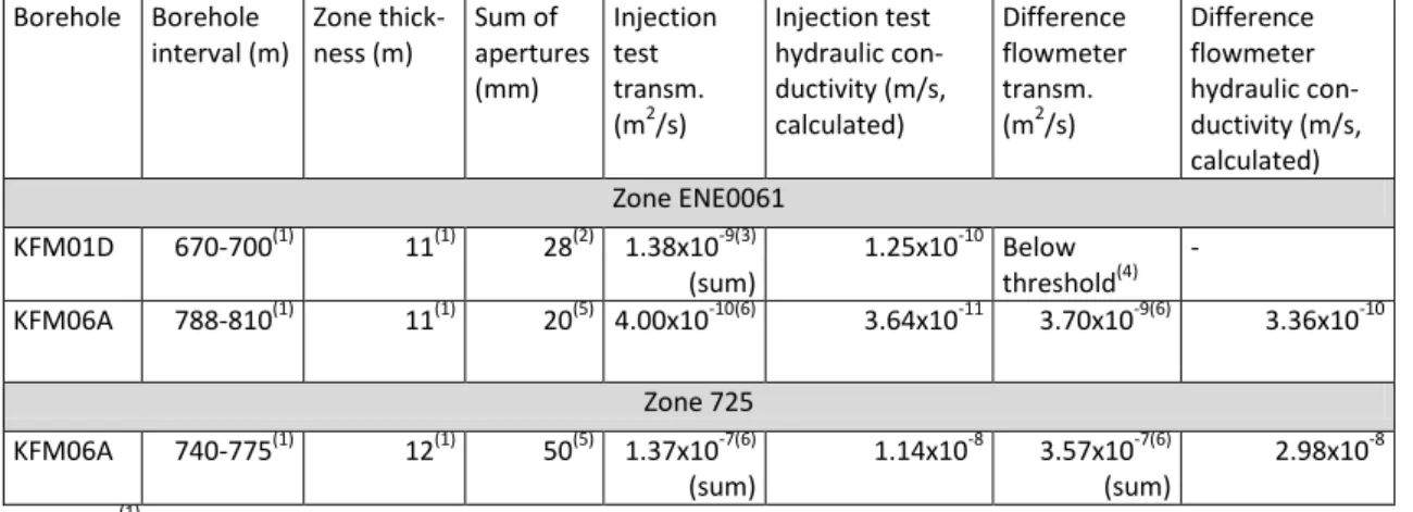
Table 1: Summary of data for calculation of permeability and porosity for Zones 61 and 725. Hydraulic conductivity values are calculated by dividing transmis-sivity by zone thickness. References are listed below the Table.

Borehole Borehole interval (m) Zone thick-ness (m) Sum of apertures (mm) Injection test transm. (m2/s) Injection test hydraulic con-ductivity (m/s, calculated) Difference flowmeter transm. (m2/s) Difference flowmeter hydraulic con-ductivity (m/s, calculated) Zone ENE0061 KFM01D 670-700(1) 11(1) 28(2) 1.38x10-9(3) (sum) 1.25x10-10 Below threshold(4) - KFM06A 788-810(1) 11(1) 20(5) 4.00x10-10(6) 3.64x10-11 3.70x10-9(6) 3.36x10-10 Zone 725 KFM06A 740-775(1) 12(1) 50(5) 1.37x10-7(6) (sum) 1.14x10-8 3.57x10-7(6) (sum) 2.98x10-8 (1)

SKB R-07-45, p. A15-72 ff. and 96 ff. (Stephens et al., 2007)

(2)

SKB P-06-132, Appendix 1 (Boremap log; Pettersson et al., 2006)

(3)

SKB P-06-195, Table 6-2, p. 32 (Florberger et al., 2006)

(4)

SKB P-06-161, Appendix 5, p. 100 (Väisäsvaara et al., 2006)

(5)

SKB P-05-101, Appendix 1 (Boremap log; Pettersson et al., 2005)

(6)

SKB P-05-165, Table 6-4, p. 64 (Hjerne et al., 2005)

See also SKB P-07-127 p. 28 and SKB P-06-56 p. 22 for correlation of Posiva flow log and boremap data for KFM01d (Teurneau et al., 2008) and for KFM06a (Forssman et al., 2006), respectively.

GROUTING - Zone 61 influences the proposed layout of the repository

(Figure 1, blue main tunnel overlaps the zone) due to a transport tunnel that is to be excavated along a part of the zone. This tunnel will be grouted if necessary. Three levels of grouting efficiency give three values of residual transmissivity after grouting (Svensson and Follin, 2010). The conductivity data calculated for Zone 61 (Table 1) show lower conductivity values than the most stringent grouting level in Table 4-3 (p. 43) in SKB R-09-19 (Svensson and Follin, 2010), i.e. between 1x10-8 m/s and 1x10-9 m/s de-pending on the hydraulic conductivity before grouting. The modeled conduc-tivity of the zones ranges from 1x10-11 m/s to about 2x10-8 m/s. Because the assumed range of permeability already includes the range possible after grouting, effects of grouting are not separately evaluated in this model anal-ysis.

(20)

4. Model construction

MODEL DOMAIN - The 2-D model constructed (Figure 3) is 2100 m wide

and 2000 m deep and is assigned a typical thickness of 11m representing the width of Zone 61 (Table 1) (and approximately representing the 12 m width of Zone 725). The repository is 1700 m wide and is modeled as 6 m high and for simplicity 11 m wide (main tunnels are planned to be 10 m wide, deposi-tion tunnels 4.2 m wide; SKB 2009), and is located at 500 m depth within the model domain. The repository is represented by a hole in the model mesh, making it possible to separately calculate inflow of water and salt into the repository from above and below with SUTRA. The depth of the model bottom is set to the location at which salinity is assumed to be 100g/L. This is the depth from which brine, which may be problematic for repository op-eration, may derive.

DISCRETIZATION AND BOUNDARY CONDITIONS - The model

domain is divided into 105 finite elements in the horizontal direction, yield-ing an element spacyield-ing of 20 m. In the vertical direction, the domain is di-vided into 25 elements above the repository and 75 elements below the re-pository with an element spacing of about 20 m. At the depth of the reposito-ry, the domain is divided into two layers of elements of size 3 m in the verti-cal direction, giving a total repository height of 6 m. The mesh refinement at repository depth allows the repository top and bottom to be represented by one row of nodes each. The repository is represented by a hole in the mesh with specified pressure boundary conditions around the perimeter of the hole. The total repository length is 1700 and the ends of the repository are 200 m from the nearest fracture zones that transect the modeled zone. In total, the finite-element mesh consists of 10540 elements and 10834 nodes (Figure 3). The effect of changing the spatial and temporal resolution of the model on the results was checked with the result that the chosen resolution gives acceptable results that do not significantly change by increasing the temporal or spatial resolution.

To simplify representations of the repository for downconing calculations, the repository volume after closure of the whole repository or part is not represented as a hole surrounded by specified pressures, but rather as a con-tiguous region of finite elements containing specified pressure nodes wher-ever the repository is still open (with pressure set equal to zero, i.e. atmos-pheric pressure). For the portions of the repository that are closed, no pres-sures are specified as a boundary condition and the pressure is calculated in the normal way by the model assuming that the closed back-filled repository has the same permeability as the surrounding bedrock.

(21)

The boundary conditions for pressure and salinity for the Base Case are shown in Table 2. In this analysis, several critical cases are considered in order to test the influence of different boundary conditions on the predicted flow fields.

INITIAL CONDITIONS - Initially, meaning, before excavation of the

repository in the model simulations, the salinity is defined to be zero at the top boundary, linearly increasing to 23 g/L at 800 m depth in the model, which is the deepest measured value at the Forsmark site. From 800 m depth to the bottom boundary at 2000 m depth, the initial salinity then increases linearly from 23 g/L to 100 g/L. The value at the bottom boundary approxi-mately agrees with the extrapolation of SKB’s modeled salinity values for the Forsmark footwall (SKB, 2008; Figure 8-46 p. 276, see also Figure 2).

Table 2: Boundary conditions for the Base Case defining pressure and the salinity of water flowing into the model.

Boundary Pressure Salinity of inflowing water where pressure is specified

Top 0 0

Bottom Hydrostatic pressure value accounting for initial salinity increase with depth

100 g/L

Left Hydrostatic pressure value accounting for initial salinity increase with depth:

m

Corresponding to initial salinity distribution:

m Right Hydrostatic accounting for salinity increase with depth,

see above

Corresponding to initial salinity distribution, see above

(22)

a)

b)

500 m

(23)

c)

Figure 3: a) Model domain and mesh (2100 m x 2000 m) showing the repository as a hole in the mesh at 500 m depth. The color shows the initial salinity distribution in-creasing from zero at the top to 10% (100 g/L) at the bottom. b) A detail of the mesh around 500 m depth shows discretization near the left end of the repository. The size of the large cells is about 20 m x 20 m. c) Model domain and mesh showing the loca-tion of observaloca-tion points used for recording time series of modeling results.

MODEL OUTPUT - Several observation points are located within the

model domain (Table 3, Figure 3c) to record details of the temporal evolu-tion of the simulated salinity as model output, in addievolu-tion to the maps of flow and salinity produced at selected times for the entire model domain. The Base Case simulation is carried out with a temporal resolution (i.e. time step) of one year for a time period of 200 years. The modelling results are record-ed every 10 years for the entire domain. Observations at the seven observa-tion points (Table 3) are recorded every year.

OTHER PARAMETERS - All other parameters needed for running the

model are listed in Table 4. Dispersivity values are for the Base Case model only; all other values are fixed for all simulations.

1-3

5-7

4

(24)

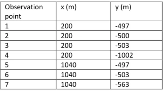
Table 3: Position of observation points. Location of the observation points in the model domain. The coordinate system has its origin (x=0, y=0) at the upper left corner of the mesh, with x increasing to the right and y upwards (Figure 3c).

Table 4: Additional model parameters.

Longitudinal dispersivity 5 m Transverse dispersivity 0.1 m

Fluid compressibility 4.47e-10 kg/(m s2) Apparent diffusivity (diffusion coefficient) of

solute in fluid

1.x10-9 m2/s Density of water ( ) 1000 kg/m3 Fluid viscosity 0.001 kg/(m s) Solid matrix compressibility 1.x10-8 kg/(m s2) Density of solid rock 2600 kg/m3 Acceleration of gravity 9.81 m/s2 Fluid coefficient of density change with

concentration

700

Density function for saline water Observation point x (m) y (m) 1 200 -497 2 200 -500 3 200 -503 4 200 -1002 5 1040 -497 6 1040 -503 7 1040 -563

(25)

5. Analysis

To study the impact of repository excavation and closure on the distribution of groundwater salinity, a sequence of events is considered in a series of simulations. Initially, there is a natural salinity distribution that is represent-ed in the model as an initial condition with the corresponding initial pressure condition that consists of a natural steady-state pressure distribution in agreement with both initial salinity and model boundary conditions. For the main sequence of simulations, at time zero, the entire repository is instantaneously opened, dropping pressures along repository walls, which were initially at high values, to zero. This initiates both downflow of groundwater from above, upflow of groundwater from below, and lateral inflow from intersecting fracture zones on the sides, as though groundwater were moving towards a horizontal pumping well. Simulation results for salt distributions that result from the flow field generated by the repository are displayed below for particular elapsed times after repository opening, up to a time of 200 years after excavation. In some cases, the flow field and salt transport are also simulated for a period of time after repository closing in order to evaluate downconing behavior. Phased excavation and closing is considered in a separate case.

The model was run through this sequence for the Base Case parameterization presented above and also for a variety of other cases, in order to explore the effect of changing various parameters and boundary conditions, in light of the uncertainty in knowledge of actual system properties. The range of pa-rameter values and conditions considered are expected to cover the full plau-sible range of possibilities for the site, such that true upconing behavior should be represented by one of the combinations considered, given the con-ceptual uncertainties of the model.

(26)

5.1 Base case

Figure 4: Salinity at time 200 years after excavation of repository for the Base Case, (with Zone 61 permeability). Colors indicate mass fraction of salt, i.e. 0.1 represents 10% salt in the water by weight. The velocity vector length is proportional to fluid velocity magnitude and flow direction directed along line away from square base of vector. The longest vector in the plot corresponds to a water velocity of 5x10-7_m/s.

Results for the Base Case parameterization representing the permeability of Zone 61 are shown in Figure 4. There is very limited movement of salt to the repository. Salinity is still slowly increasing even after 200 years of a com-pletely open repository and the salt content has increased from about 1.5% to only about 2.1% at the repository center, where it is greatest. At the sides of the repository, the salt content of the inflowing water has hardly changed at all, remaining at 1.5% (from 1.45% to 1.52%). In contrast, Figure 5 (lower panel) shows a breakthrough of water with a salt content that reaches steady-state after only 25 years, with the rather high salinity of 10%, for the case representing the permeability for Zone 725.

(27)

Figure 5: Salinity at time 25 years after excavation of repository (above), for the Base Case (with Zone 725 permeability) showing upconing. Salinity at time 10 years after closure of the repository (below), showing downconing. The dashed line indicates the location of the closed repository. Colors indicate mass fraction of salt, i.e. 0.1 repre-sents 10% salt in the water by weight. The velocity vector length is proportional to fluid velocity magnitude and flow direction directed along line away from square base of vector. The longest velocity vectors for the upconing and downconing case corre-spond to 8 x 10-5 m/s and 5 x 10-7 m/s for the upconing and downconing case, re-spectively.

(28)

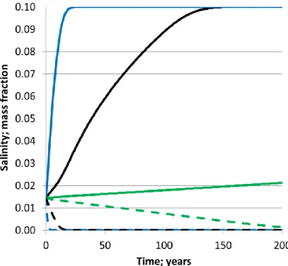
Figure 6: Breakthrough curves for the Base Case for observation point 6 (Figure 3c) in the mid-bottom of the repository (full lines) and observation point 5 in the mid-top of the repository (dashed lines). Breakthrough shown for permeability of Zone 61 (6.7x10-18_m2_{; green lines), Zone 725 (1.8x10}-15_m2_{; blue lines) and for a case with}

intermediate permeability (1.3x10-16 m2; black lines).

As occurs for Zone 61, the salinity at the ends of the repository for the case of permeability representing zone 725 is also nearly unchanged. This is ex-pected since the repository draws the water from the closest boundary, and the boundary condition concentration at repository depth has been set equal to the initial condition at the repository. Breakthrough curves for points above and below the repository center for the permeability cases shown in Figure 5, as well as for an intermediate permeability of 1.3x10-16 m2, are shown in Figure 6.

The simulated influx of water to the repository from the zone amounts to 0.2 m3/day for the low-permeability zone and 45.7 m3/day for the

high-permeability zone after 200 years. The simulated amount of salt entering the repository is 2 kg/day and 930 kg/day, respectively, at time 200 years. For Zone 725, the amounts at 25 years and at 200 years are equal because a steady state is already reached at 25 years. For both cases, about 60% of total inflow occurs to the top of the repository and about 40 % occurs along the floor of the repository.

(29)

The post-closure downconing for the Zone 725 case (Figure 5, upper panel) occurs relatively quickly. By 10 years following closure, the cone has sunk-en over 100 m (Figure 5-upper panel) and it continues to sink further. It can be noted that the water at the closed repository is fresher during downconing than it was under the initial conditions, because the sinking body of previ-ously-upconed saltwater causes a downflow of freshwater from the top sur-face of the model (Figure 5).

5.2 Effect of topography and different

boundary conditions

In these variations, the impacts of topography and differing lateral and bot-tom boundary conditions on upconing are investigated. Topographic undula-tion and trend in surface hydraulic head are neglected in the Base Case wherein a constant pressure of zero is assigned at the top boundary, repre-senting a flat water table. A case was run explicitly considering the topogra-phy as a tilted sinusoidally-undulating surface with the mean height varying 10 m across the domain, a wavelength of 300 m, and with peak-to-peak am-plitude of 6 m. For freshwater calculations without a repository, this yields a flow field with very low groundwater velocities, due to the low transmissivi-ty of the modeled structure and the small gradients. (A higher transmissivitransmissivi-ty of the soil and uppermost rock is not accounted for in the model because this is not expected to significantly impact the flows being studied at depth.) The simulation with topography present and with initial salinity as in the Base Case displays no observable influence of the topography on the flow field compared to the case without the topographic variation (result not shown). The Base Case has specified hydrostatic pressures at the left, right and bot-tom boundaries that are in equilibrium with the initial saltwater distribution. This represents the situation in which water from transecting structures can laterally enter/exit the studied sub-vertical structure. A variant simulation was also run with closed vertical subsurface boundaries, i.e. with no flow boundaries along left and right sides, representing the case where no lateral flow occurs from/to transecting structures. Another variant simulation was run with hydrostatic conditions that were specified for the Base Case at the left and right boundaries, but with a no-flow boundary at the bottom. The latter case represents the situation in which the bottom of the studied struc-ture is closed to flow and all flow enters/exits from transecting strucstruc-tures. Salinities and breakthrough curves for these simulations are shown in Figure 7 and Figure 8.

(30)

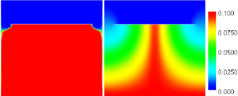
Figure 7: Salinity at steady state for no flow boundaries at the sides (left) and closed bottom boundary (right). Colors indicate mass fraction of salt, i.e. 0.1 represents 10% salt in the water by weight.

Figure 8: Breakthrough curves for different boundary conditions for observation point 6 in the mid-bottom of the repository using the intermediate permeability value shown in Figure 6. Hydrostatic subsurface boundaries (black line – Base Case), no flow lateral boundaries (green line), and no flow bottom and hydrostatic lateral boundaries (blue line).

The amount of water entering the repository is rather similar for the three cases, with the closed lateral case being about 30% lower and the case with the closed bottom about 2%. Compared to the Base Case, the salt mass in-flow rate for the closed lateral case is about 25% lower and for the case with the closed bottom is about 17% lower. There is a large salt intrusion for the case of closed lateral boundaries with high concentration throughout the repository (Figure 7 left panel). However, it should be noted that although all fluid in the rock below the repository becomes highly salinized, salt influx to

(31)

the repository is actually smaller than for the Base Case and the case with closed bottom, because the water inflow to the repository from below is low-er than for these cases.

For closed side boundaries, there is more widespread intrusion of high salini-ty to the repository at steady state for all fracture zone permeabilities. The evolutions of salinity at the repository center are similar for the Base Case with all open boundaries and the case with closed side boundaries (compare in Figure 8), but the spatial distributions are different with more widespread upconing in the closed boundary case (compare Figure 5- lower panel with Figure 7-left panel). For a closed bottom boundary, the amount of intrusion is decreased relative to the Base Case, noting that the upconed area in Figure 7-right panel is narrower than in Figure 5- lower panel. In fact, the upconed area decreases with higher permeability when the bottom boundary is closed (simulation results not shown), providing the possibility of a situation where-in there is no significant upconwhere-ing from directly below the repository, alt-hough zone transmissivity is high.

5.3 Effect of initial salinity distribution

As there is only limited information on the current distribution of subsurface salinity at the Forsmark site, four initial salinity distributions were tested to explore their effect on possible upconing and downconing behavior. These simulations were run with a permeability of 1.3x10-16 m2, a value between the values for zone 61 and 725. In the first simulation, the initial salinity is modeled as specified above for the Base Case, i.e. linear increase from zero to 2.3% from the ground surface to 800 m depth and then linear increase to 10% at 2000 m depth. In a second simulation the increase to 800 m depth is the same but the value is then held constant at 2.3% down to 2000 m. The salinity of water flowing into the domain at the bottom is still set to 10%. In the third case, the initial salinity distribution is the same as for the other cas-es down to 800 m and then it linearly increascas-es to 7.5% at 2000 m depth. In the fourth case, the same initial salinity distribution is applied down to 800 m and then the salinity increases linearly to 10% at 1500 m depth. Below 1500 m the salinity is constant at 10%.

(32)

Figure 9: Initial salinity distributions for checking the effect of the initial salinity distri-bution. The left upper panel shows the salinity distribution linearly increasing from zero to 2.3% from the ground surface to 800 m depth (deepest measurement at For-smark) and then linearly increasing to 10% at 2000 m depth, corresponding to Figure 3. In the upper right panel the increase to 800 m depth is the same but the value is then held constant at 2.3% down to 2000 m. The lower left panel shows an initial salinity distribution as for the other down to 800m and then linearly increasing to 7.5%. The lower right panel shows the same salinity distribution down to 800m and the linearly increasing to 10% at 1500 m depth. Below 1500 m the salinity is constant at 10%. Colors indicate mass fraction of salt, i.e. 0.1 represents 10% salt in the water by weight.

Results show that a situation with brine entering the repository, as shown in Figure 5 (lower panel), is reached after about 145 years for the case with the salinity increasing to the bottom of the domain. In the case with constant salinity below 800 m, the salinity in the water entering the repository in-creases for about 15 years from 1.6% to 2.3% and then is constant at this value until about 65 years when the salinity starts increasing again and at about 185 years reaches 10% (see Figure 10). For the case with a maximum salinity of 7.5% at 2000 m depth, the time until the maximum salinity reach-es the repository is about 140 years. For the case with the maximum salinity being initially at 1500 m depth, the brine reaches the repository after about 90 years and the upconed zone is wider than for the other cases (not shown).

(33)

Figure 10: Salinity versus time for the four simulation cases shown in Figure 9 at observation point 6 as defined in Table 3, which lies at the bottom middle of the re-pository. Initial salinity equal to the Base Case (initial salinity shown in upper left panel in Figure 9; black line), initial salinity constant salinity below 800 m depth being 2.3% (initial salinity shown in upper right panel in Figure 9; red line), initial salinity as for the other cases down to 800 m depth and then increasing linearly to 7.5% at 2000 m depth (initial salinity shown in lower left panel in Figure 9; yellow line), and initial salinity equal to other cases down to 800 m depth and then increasing linearly to 10% at 1500 m depth (initial salinity shown in lower right panel in Figure 9; violet line).

5.4 Effect of porosity and permeability

Two of the most important hydraulic parameters of the fracture zones, poros-ity and permeabilporos-ity, are uncertain. Figure 6 shows that the permeabilporos-ity has a pronounced effect on the saline water intrusion to the repository. The val-ues vary only about 2 orders of magnitude but the result is that either no intrusion of highly saline water occurs at all, or a rather quick intrusion oc-curs after about 20 years. Simulations based on a range of values of these parameters were run to evaluate the sensitivity of upconing behavior to these controls. The results are shown in Table 5. It is observed in the table that the order of the ratio of porosity to permeability is exactly the same as the order of the breakthrough times. This would be expected for the situation in which there are insignificant density forces, in which groundwater flow is driven only by differences in hydraulic head, because, in Darcy’s Law, the ratio (permeability/porosity) is the parameter that multiplies the gradient in hy-draulic head when calculating fluid velocity. Thus, irrespective of the

(34)

partic-ular boundary conditions, the speed of upconing and timing of salt arrival at the repository depends only on the ratio of porosity and permeability, and not on either parameter independently.

Table 5: Results with ranks of order of porosity-permeability ratio and of simu-lated 100g/L salinity breakthrough (in years). All simulations have base-case parameter values except for porosity and permeability.

Order (Porosity/ Permeability) Order break-through time Porosity (-) Permeability (m2) (Porosity/ Permeability) (m-2) Time to break-through of 100 g/L salinity (years) 1 1 9.00x10-04 1.30x10-14 6.92x10+10 5.0 2 2 9.00x10-04 1.30x10-15 6.92x10+11 21.0 3 3 1.40x10-03 1.80x10-15 7.78x10+11 25.0 4 4 4.00x10-04 1.30x10-16 3.08x10+12 71.0 5 5 9.00x10-04 1.30x10-16 6.92x10+12 149.0 6 6 4.00x10-03 1.30x-16 3.08x10+13 not reached; 0.02 reached at 46 years 7 7 9.00x10-04 1.30x10-17 6.92x10+13 not reached; 0.02 reached at 83 years 8 8 9.00x10-04 6.70x10-18 1.34x10+14 not reached; 0.02 reached at 163 years

5.5 Effect of spatial trends and

heteroge-neity

The Base Case and the other cases shown above all assume that the defor-mation zone can be represented in the model by a feature that has a homoge-neous permeability and porosity. Clearly, this is a simplifying assumption and therefore, the effect of spatial trends and heterogeneity in the primary hydraulic parameters (permeability and porosity) of the simulated fracture zone is explored in a few simulations.

DEPTH DEPENDENCE - The depth dependence of permeability and

po-rosity are calculated by the equations suggested by SKB (Svensson and Fol-lin, 2010). The transmissivity depth dependence is expressed as (eq 2-1 Svensson and Follin, 2010; p. 15):

⁄ ₍₁₎

in which T is transmissivity (m2/s), y (m) is the depth coordinate (negative below ground) and k (m) is a parameter that expresses the depth interval that yields an order of magnitude difference in transmissivity.

(35)

√

(2)

Inserting equation 2 into equation 1 yields: √ ⁄

(3)

with the coefficient 0.25 having the unit (s), const (m2/s)being a constant that is determined based on site data. This is obtained by dividing equation 3-2 of Joyce et al. (2010; p. 30) by the borehole interval length [m] observed for the deformation zone to obtain porosity from fracture aperture. Since the perme-ability (m2) is equal to the transmissivity (m2/s) multiplied by a factor 107 ms divided by the zone thickness (m), the transmissivity value can be replaced by the permeability in the equations. The constant in the porosity equation can be calculated by inserting the values known for a certain depth. In prin-ciple, the constant could also be calculated from the transmissivity at depth zero, but in the other modelling cases considered here, the relation between porosity and transmissivity was not used, since both are independently calcu-lated based on measured variables, i.e. transmissivity from borehole tests and the porosity from summing the detected apertures in the zones (as explained previously). For the cases with depth-dependent transmissivity considered here, the value of k (in Equation 1) is chosen as 500 m and the resulting T(0) = 5.96x10-14 m2/s is calculated based on data for zone 725 at a depth of 760 m (see above). For the case with depth-dependent porosity, this yields const = 0.34 (m2/s). The depth dependence (Equation 1) is parameterized for the current analysis in a way that gives the same permeability at the depth of measurement (at about 760 m for Zone 725). Below this depth, the permea-bility is lower and above that it is actually higher than for the base case. For the case in which the porosity is calculated from Equation 3, the porosity is lower below the measured point and higher above.

In Figure 11 results are shown for two cases of spatial trends. Both include depth-dependent permeability and one also includes depth-dependent porosi-ty. It can be seen that upconing occurs much more quickly should both per-meability and porosity decrease with increasing depth in the zone. In Figure 12, the breakthrough curves at the mid bottom of the repository are shown for these cases, as well as for the Base Case with constant permeability, with and without depth-dependent porosity according to Equation 3.

(36)

Figure 11: Salinity after 100 years in Base Case model. Left panel case has depth-dependent permeability according to SKB’s equation (equation 1) and k=500 m and permeability of zone 725 at the measured depth of 760 m. The right panel case has the same depth-dependent permeability and additionally, depth dependent porosity (equation 3). Colors indicate mass fraction of salt, i.e. 0.1 represents 10% salt in the water by weight.

Figure 12: Salinity versus time for the Base Case model and permeability of zone 725 (black line) and the Base Case model with added depth-dependent permeability according to SKB’s equation (equation 2) and k=500 m and permeability of zone 725 at the measured depth of 760 m (blue line). The red line shows results for the same depth-dependent permeability and additionally, a depth-dependent porosity (equation 3; const=0.34 m2/s and k=500 m). The green line shows the Base Case model with constant permeability of zone 725 with depth dependent porosity (equation 3; const=0.34 m2/s and k=500 m).

(37)

HETEROGENEITY - Arbitrary heterogeneous permeability fields are

as-sumed for the zone, as illustrated in Figure 13. In the first heterogeneous case, heterogeneity in permeability is represented as a pattern of high and low permeability patches via a sine function multiplied by cosine function of log10(permeability). This leads to a span in permeability, k, over about 6

orders of magnitude, (1x10-14 m2 to 1x10-20 m2; Equation 4 and Figure 12 with left scale, which shows –log10(permeability)). The distance between

adjacent max and min permeability values is about 160 m (π/0.02 m-1) in both x and y directions. This can perhaps roughly represent spatial variabil-ity due to fracture aperture and aspervariabil-ity variation within the fracture planes of the zone. The geometric mean of the permeability is taken from the Base Case with permeability of zone 61.

(4)

In a second heterogeneous case, the heterogeneity in permeability is also represented using the product of a sine function and a cosine function, but one that spans only approximately 2.5 orders of magnitude (equation 5 and Figure 12 with right scale, which shows -log10(permeability)). The spatial

distance between max and min permeability values is the same as in the first distribution.

(5)

Porosity is held constant for both heterogeneous fields and other model fac-tors are the same as in the Base Case.

Figure 13: Distribution of permeability in cases with heterogeneity. The coloring ex-presses -log10(permeability). The left color bar represents the Base Case with

per-meability of zone 61 (with lower mean and higher variance of perper-meability) and the right color bar of zone 725 (with higher mean and lower variance of permeability).

(38)

Figure 14: Salinity distributions for heterogeneous permeability patterns. After 200 years for Zone 61 case with lower permeability and higher variance using equation 4 (left panel). Salinity distribution after 10 years and for Zone 725 case with higher permeability and lower variance using equation 5 (right panel). Colors indicate mass fraction of salt, i.e. 0.1 represents 10% salt in the water by weight.

Salinity results from these simulations are shown in Figure 14. In the first heterogeneous case with mean permeability corresponding to Zone 61 and higher permeability variance, no highly saline water reaches the repository at the end of the simulation at 200 years due to the overall lower value of per-meability. Upconing occurs preferentially along paths that follow the regions with the greatest permeability. In the lower permeability pockets, the salinity hardly changes at all during the 200 year simulation. For the second hetero-geneous case with a mean permeability corresponding to Zone 725, about 2 orders of magnitude higher than the Zone 61 case, and with lower permeabil-ity variance, the highly saline water reaches the repository after only 10 years and a steady state is reached at about 35 years. Also in this case the upconing occurs preferentially along paths of high permeability while avoid-ing patches of low permeability (Figure 14 right panel). Should groutavoid-ing have been done around the repository tunnels, the intersections of the highest hydraulic conductivity paths would have reduced conductivity, decreasing the connection of the low tunnel pressure to the bedrock and probably reduc-ing the rate of upconreduc-ing and breakthrough.

5.6 Effect of phased tunneling

To see how phased tunneling may influence upconing behavior, a simulation was run in which only a part (100 m of tunnel length) of the entire repository is open at any given time. This was modeled by changing the internal speci-fied pressure boundary condition along repository walls at 30, 60, and 90 years in a way such that different portions of the open repository are repre-sented. Thus three different sections were opened and closed in sequence. This may be considered as representing three phases in repository operation. In reality, the opening and closure of the tunnels will follow a more

(39)

elabo-rate pattern, most likely with smaller distances between the tunnel portions that are opened and closed. Figure 15 shows the locations of the open reposi-tory sections (small red horizontal bars) and presents the simulated salinity distribution at 30, 40, 60, and 90 years after the first excavation was begun. The results show the situation just before each tunnel section is closed (ex-cept at 40 years) and thus the maximum of upconing for each open section. The result for 40 years illustrates how the existing upconed saltwater is held at more or less the same depth even when the water is drawn into a newly opened section.

It can be seen that the upconing through this structure reaches each open section of the repository before each section is closed, with high salinities reaching the open part of the repository.

Figure 15: Salinity distribution for a partly open repository with phased tunneling. Permeability is that of Zone 725. The open part of the tunnel is represented by a specified pressure of zero spanning five elements horizontally and two elements vertically, and is thus, 100 m wide and 6 m high. Each section is held open for 30 years. The specified pressure boundary condition locations were changed at 0, 30, 60, and 90 years. Results are shown after 30 years (upper left), 40 years (upper right), 60 years (lower left), and 90 years (lower right). Colors indicate mass fraction of salt, i.e. 0.1 represents 10% salt in the water by weight.

(40)

5.7 Effect of higher dispersion

The dispersivity values used for most simulations (5. m and 0.1 m for longi-tudinal and transverse dispersivities, respectively; Table 4) are not well-known values for solute transport in fracture zones and few field measure-ments have been made at the scales of transport that occur during upconing. Running a simulation with dispersion (i.e., longitudinal and transverse dis-persivities) increased by one order of magnitude gives essentially the same breakthrough curves at the bottom center of the repository (not shown). High concentrations are reached at about the same time, but small late-term con-centration increases occur, and steady state occurs a few tens of years later than for lower dispersion. Thus, given that the important point is the ques-tion if highly salinity water reaches the repository quick enough to adversely impact the resaturation of the buffer, higher dispersivity has negligible im-pact on the upconing process.

(41)

6. Discussion of results

APPROACH - Because the model is very much a simplification of the real

conditions and because values of important physical controlling parameters are to a large extent uncertain, this analysis considers variations of both pa-rameter values and hydrologic conditions, in order to determine important factors that control the upconing behavior at the Forsmark site. Also, this approach defines the range of possible upconing behaviors that might be expected to occur at the site.

ASSUMPTIONS - Several key simplifying assumptions that affect the Base

Case modelling results were discussed earlier. Three not yet discussed are: (1) The zone is represented from the surface down to 2000 m as being con-tinuous, at least in view of its permeability and porosity on a scale relative to the discretization of the model domain. This is a basic requirement for the process of upconing to occur; there must be a continuous hydraulic path between the saltwater source and the repository.

(2) A constant pressure boundary condition was employed at the ground surface in this analysis. It is possible that the modeled inflow of water from this boundary might be larger (or smaller) than the net infiltration that is linked to the precipitation at the site. In reality, a situation with recharge less than modeled inflow would lead to water-table drop, which was not mod-elled. Both a saturated zone extending only part-way to the ground surface and a no-flow boundary at the top of the domain may affect saltwater up-coning.

It is possible to evaluate the impact these situations would have on upconing, as follows. Upconing is a simple process primarily controlled by Darcy's Law in the case where the hydraulic gradient imposed by the repository overwhelms the buoyancy forces. In this case, the only factors that control upconing are the pressure (i.e. head) difference between repository and salt-water source zone, the distance to the source of saltsalt-water, and the permeabil-ity and porospermeabil-ity of the flowpath that connects the source with the repository. This means that a closed model top (no-flow boundary) will not change the pressure in the repository, so it will not much affect saltwater movement from a source at the bottom of the section. The fact that the repository pres-sure itself controls the head gradient to any saltwater source makes the con-trols on upconing clear. It is possible that the saltwater inflow to the top of the tunnel can change when the model top is closed because some saltwater could move upwards around the ends of the tunnel and enter the low-pressure zone above the repository, finally discharging into the top of the repository. However, much less saltwater could enter this way than from

(42)

below, so this is expected to be a minor effect. If the top 500 m just above the repository were partly or fully drained, this additional inflow would stop completely, making it even less important.

Further, there are connections to the nearby Baltic Sea in at least some For-smark boreholes and the upper part of the system has relatively large trans-missivity that would enhance connections to shallow water sources. This could lead to recharge of Baltic seawater, in addition to local freshwater recharge, which would limit such a water-table drop, but would deliver brackish water to the repository from above. Such calculations have not been carried out in this study.

The rock, of which the fracture zones are a part, is overlain by Quaternary deposits, which have considerably different hydraulic characteristics and likely greater porosity and thus groundwater storage than the zones. Such deposits are neglected in this study as a specific geologic layer, but these provide a source of water similar to the fixed pressure used in this study, so their effect is already included.

(3) The impacts of variations of some types of conditions within zones that intersect the modeled zone have not been directly considered in this model-ing analysis. In the case where the intersectmodel-ing zones are more transmissive than the one modeled, more upconing could occur in these zones than in the modeled zone, and therefore the salinity at the intersections should also be elevated, forming a changing lateral boundary condition for the zone being modeled. In this particular case, highly saline groundwater could flow to-ward the excavation from the sides of the modeled region, rather than from the bottom. For this situation, the present approach is conservative, implying lower brine concentrations in the repository than would occur should en-hanced upconing occur in transecting structures.

(4) The effects of the heating imposed by the spent nuclear fuel canisters are not accounted for explicitly in the simulations. At repository level the tem-perature of the rock is expected to increase with max 30 degrees centigrade about 50 years after canister emplacement (SKB, 2011). The larger the dis-tance from the canisters the smaller the heating effect. A 30 degree tempera-ture increase will change the density of the water and its viscosity signifi-cantly. The results of this study indicate that it is the change in pressure that mainly drives the upconing and that density effects are not central. Thus the temperature effect on the water density should not change the main results of the study. An increase of 30 degrees centigrade will yield a 50% smaller viscosity, and thus conductivity, around the repository compared to the value used in the modelling. The modeled permeability covers several orders of magnitude and thus this effect should not change the overall conclusions of the study.

(43)

(5) In the downconing calculations it is assumed that the repository has no effect on downward flow through the repository. The bentonite should have a lower permeability than the fracture zone modeled, thus in the 2-D model the flow through the repository may be hindered. In 3-D this effect may be less pronounced. In any case, there is a possibility that the downconing could be slowed by the backfilled repository in comparison to the results indicated by the model.

6.1 Base case

The three Base Case simulations indicate that, should porosity be constant throughout the vertical fracture zone considered, it is the permeability that has a large influence on the occurrence of intrusion of highly saline water into the repository within 200 years and the timing of this occurrence. The permeability values and the other parameter values for these simulations are derived from the results of SKB’s site investigations at Forsmark, and these values are believed to represent the range of conditions that can be encoun-tered at the site. The model results thus indicate that, at parts of the reposito-ry that are intersected by relatively high permeability zones, upconing may occur quickly following excavation. In the modeled case with the highest permeability, water with high salt content rises 1500 m to the repository within only two decades after excavating the repository.

In a relatively high-permeability zone, downconing also occurs quickly. The repository fluid freshens due to inflows from above, drawn in by the drop-ping volume of saline water below the repository. In contrast with upconing, which is driven almost exclusively by hydraulic forces due to the low pres-sure in excavated tunnels, downconing is driven exclusively by buoyancy forces arising from differences in fluid density.

The rather quick sinking of the upconed saltwater in the high permeability case raises the question of the stability of the assumed initial conditions of the model. Modeling the Base Case with permeability for Zone 725 without a repository, and thus only studying the evolution from the assumed initial conditions, indicates that the salinity field slowly moves downwards (not shown). Thus the initial condition is not at steady state with respect to the boundary conditions applied. A comparison of this simulation with the downconing behavior shown in Figure 5 indicates that the sinking saline cone moves considerably faster than the dropping initial salinity distribution, and thus draws a higher flux of fresh water downwards than does the evolu-tion of the initial condievolu-tions. To get a more or less stable (i.e. steady-state) salinity profile that increases with depth, as indicated by field data, the per-meability must either be very low (as in the case of Zone 61) or there must be a source of salt, either internally or through transport of salt entering the system through the model boundaries. Alternatively, the current salinity distribution at Forsmark may simply not be in a steady state. The question of