1
VIX Futures Calendar Spreads
*
AI JUN HOU LARS L. NORDÉN June 27, 2017 A VIX futures calendar spread involves buying a futures contract maturing in one month and selling another one maturing in a different month. VIX futures calendar spreads represent a daily turnover above 500 million dollars, or roughly 20% of the total VIX futures trading volume. A calendar spread trade is a bet on the change in the slope of the volatility term structure. We find that speculation, rather than information about changes in the slope of the volatility term structure, is driving calendar spread trades. On average, a calendar spread costs a little less than $100 (about 15 basis points). If settled at the end of the trading day, 43% of the calendar spreads are profitable. * Ai Jun Hou and Lars L. Nordén are grateful to the Jan Wallander and Tom Hedelius foundation and the Tore Browaldh foundation for research support. We thank Björn Hagströmer and Caihong Xu for valuable comments and suggestions. Contact: Ai Jun Hou, Stockholm Business School, Stockholm University, (Email) aijun.hou@sbs.su.se, (Tel) +46-8-6747097; and Lars L. Nordén, Stockholm Business School, Stockholm University, (Email) lars.norden@sbs.su.se, (Tel) +46-8-6747139.
2 1. Introduction In a complete markets’ setting, derivatives are important vehicles for hedging investment portfolios against unfavorable outcomes (Black and Scholes, 1973; Cox and Ross, 1976). In addition, when markets are incomplete, e.g., when volatility is stochastic or asset prices exhibit jumps, derivatives can complete the markets and improve efficiency (Ross, 1976; Breeden and Litzenberger, 1978; Bakshi and Madan, 2000). Liu and Pan (2003) show that by adding derivatives to a portfolio of equity and bonds, investors can improve the portfolio performance and get exposure to volatility risk and jump risk in the equity market.
An equity market investor can get exposure to volatility risk by trading a variety of volatility sensitive assets like S&P 500 variance swaps, S&P 500 index option straddles, or VIX futures and options.1 To span the volatility risk an investor needs to use the term structure of volatility. For this purpose, Egloff, Leippold, and Wu (2010) advocate the use of variance swaps, while Lu and Zhu (2010) prefer VIX futures. Johnson (2016)
demonstrates that the slope of the volatility term structure captures all information about the price of volatility risk, and predicts returns of volatility sensitive assets.
This paper adds to the literature by arguing that calendar spreads in VIX futures offer a way to trade the slope of the volatility term structure.2 A VIX futures calendar spread involves buying a futures contract maturing in one month and selling another one
1 VIX futures trade on the CBOE Futures Exchange (CFE). CBOE Holdings, Inc. is the holding company for the Chicago Board Options Exchange (CBOE) and the CFE. CBOE Holdings offers trading in S&P 500 index options (SPX) and options and futures on the CBOE Volatility Index (the VIX). The VIX is the expected annualized volatility (in %) of the S&P 500 index over the subsequent 30 calendar days. For more information about the VIX, see the CBOE micro site on VIX at http://www.cboe.com/micro/vix/vixintro.aspx
2 Egloff, Leippold, and Wu (2010) make a similar argument when they find it optimal to combine an equity investment with a long position in short-term variance swaps and a short position in long-term swaps, or vice versa. In essence, their recommended position is a calendar spread in variance swaps.
3
maturing in a different month. For example, in the March/April spread, traders will buy
March futures while simultaneously selling April futures (or vice versa). With a calendar spread, a trader profits from the change in the price differential of the two contract months. A trader is entering a long delta calendar spread by buying the short-maturity and selling the long-maturity futures contract, while a short delta calendar spread is when
the trader is selling the short-maturity and buying the long-maturity contract.
We identify VIX futures calendar spreads directly in our data. A VIX futures calendar spread is tradeable as a spread trade package in the CFE trading system. According to CFE rules, a spread order is part of a strategy to simultaneously buy, sell, or both buy and sell,
at least two futures contracts in the same underlying asset, with different expiration dates.3 In our sample, spread trade strategies make up for roughly 30% of the total VIX futures trading volume, while the remaining 70% of the volume results from regular individual futures trades. The calendar spread is the most common strategy, and it represents around 70% of the total spread trade volume (or 20% of the total VIX futures
trading volume). On a daily average basis, calendar spreads turn over more than 500 million dollars.
Johnson (2016) finds that the slope of the volatility term structure predicts returns of volatility sensitive assets, including VIX futures returns, in a statistical sense. In this paper, we go beyond statistical predictability and investigate if actual trading in VIX futures calendar spreads carry information about the future term structure of volatility. In
addition, we analyze if speculation is driving trading in VIX futures calendar spreads. Specifically, we analyze if informed traders, who possess information about the slope of the volatility term structure, or uninformed speculators, who follow strategies based on
4
recent movements in the slope, are using VIX futures calendar spreads. In the former case,
the information will become common knowledge through trading and futures prices will adjust accordingly. Thus, spread trades will precede changes in the volatility term structure. In the latter case, movements in the term structure slope will lead trading as the spread traders are acting upon recent term structure movements.
To measure the information content of VIX futures calendar spread trades we use the empirical framework of Hasbrouck (1991). Here we apply a bivariate VAR model of the intraday dynamic relationship between calendar spread returns (representing movements in the slope of the volatility term structure) and calendar spread trades.
Specifically, we relate returns to calendar spreads using nearby and next-to-nearby VIX futures contracts to the corresponding net calendar spread trade volume (buyer-initiated volume less seller-initiated volume). The VAR model enables an analysis of not only whether spread trades affect calendar spread returns, but also reversely, if changes in the term structure slope drive the spread trades.
Our results indicate that changes in the volatility term structure drive trading in calendar spreads, and the relationship is negative. Accordingly, a flattening of the term structure slope induces spread traders to prefer short delta spread strategies to long delta strategies, and is consistent with the idea that spread traders speculate in response to changes in the slope. A positive calendar spread return equal to one tick, i.e., a 0.05 index-point or $50 change, causes a subsequent negative net calendar spread volume of the
magnitude 12 contracts within an hour. However, we find no support for the hypothesis that calendar spread trades are informative.
Whether trading for information or speculative purposes, calendar spread traders care about how costly and profitable these strategies are. For the calendar spreads using
5
nearby and next-to-nearby VIX futures contracts, we measure each calendar spread’s
trading costs with the sum of the effective spreads for both futures legs. Each effective spread equals the difference between each futures transaction price and the midpoint between the best bid quote and the best ask quote, prevailing at the time of the trade. An average calendar spread costs about 15 basis points, or less than $100 to trade. For
corresponding regular single futures trades, not using the facility of a spread trade package, the average costs are about twice as high. We estimate short-term gains and losses on the VIX futures calendar spread, both with an intraday five-minute holding period, and by marking the strategy to market at the end-of-day futures settlement. Five minutes after a calendar spread trade, on average, futures prices move in an unfavorable direction by 2.5 basis points, or $15.5. In addition, after considering the initial transactions costs, almost 80% of the calendar spreads are losing money over a five-minute period, which is again consistent with calendar spread trades not carrying information. If strategies are settled at the end of the trading day, the average calendar spread gain before transactions costs is two basis points or $9. Interestingly, short delta calendar spreads generate an average gain equal to 8.3 basis points ($62.6) and long delta spreads produce an average loss of 4.4 basis points ($46.7). Adjusting for transactions costs, 43% of all calendar spreads are profitable, while almost 60% of the short delta spreads are profitable and only 30% of the long delta spreads gain money. Although futures calendar spreads are popular among traders in the VIX futures market, and probably in other futures markets, very few studies of these strategies exist. Frino and McKenzie (2002) analyze the pricing of calendar spreads in stock index futures close to contract maturity. They hypothesize that calendar spreads carry mispricing when one of the futures contracts in the spread is close to maturity. According to their hypothesis,
6
the mispricing mechanism is associated with futures traders' rollovers between the
nearby contract and a deferred contract. In an empirical analysis of end-of-day individual futures transactions data, the authors find evidence in favor of their hypothesis. While we access information about spread trades, Frino and McKenzie (2002) cannot disentangle spread trades from regular futures trades. Frino and Oetomo (2005) and Frino, Kruk and Lepone (2007) investigate if individual futures trades that are part of trade packages have price impacts. They find little evidence that futures trades contain any information. Thus, they conclude that uninformed liquidity traders are executing futures trades. The authors define trades from the same
trader's account, in the same direction (e.g., buying), and if they are executed without a one-day break, as belonging to a package. Our primary focus is on calendar spread trades, whereas both Frino and Oetomo (2005) and Frino, Kruk and Lepone (2007) classify spread trades, which contain both long and short futures positions, as individual trades - not part of packages in their analyses. In a related study, Fahlenbrach and Sandås (2010) carry out an investigation of option trading strategies in the FTSE-100 index market. Similar to us, they are able to identify strategies through some key features of their data, including a flag for strategy trades. In their sample, about 37% of all option transactions occur within as many as 44 distinct option strategies. Fahlenbrach and Sandås (2010) discover that volatility-sensitive option strategies contain information about future index volatility, while directional strategies hold no information about future returns. In addition, volatility strategies are on average profitable, while directional strategies are not. In several papers, Chaput and Ederington (2003; 2005; 2008) investigate different option trading strategies, including spreads, using data on large option trades in the Chicago
7 Mercantile Exchange’s market for Options on Eurodollar Futures. Their data were actually assembled by hand by an observer at the periphery of the Eurodollar options and futures pits with instructions to record all option trades of 100 contracts or larger. 2. VIX futures market structure, data and calendar spread identification The CFE introduced VIX futures in March 2004. On any particular day, the VIX measures
the expected annualized percentage volatility of the S&P 500 index over the next 30 calendar days. In this respect, the VIX corresponds to the implied volatility of S&P 500 index options. It is widely recognized as an important forward-looking indicator of uncertainty faced by financial market participants.
The CFE offers several different ways to trade VIX futures. Regular futures trades occur within an electronic limit order book. Orders allowed in the VIX futures limit order book include both liquidity-consuming market orders and liquidity-providing limit orders. The contract multiplier is $1,000 for each VIX futures contract. For an order or trade, the minimum price increment is 0.05 index points, which corresponds to a $50 contract value
per tick. CFE also manages a separate trading facility for spread trades for combinations of VIX futures contracts with different maturities. Spread trades must adhere to the following distinct futures spread trade strategies: (i) two-legged spreads with a relation between the number of futures contracts in the first leg is 1:1 or 1:2 to the number of contracts in the second leg; (ii) three-legged spreads with a relation 1:1:1 or 1:2:1; and (iii) four-legged spreads with a relation 1:1:1:1. For each futures leg of a spread trade, the minimum price increment is 0.01 index points ($10 value per tick).4 4 It is also possible to trade VIX futures using the Trade at Settlement (TAS) feature at CFE. At any time during exchange trading hours it is possible to enter limit orders in the TAS limit order book, which is distinct from the regular VIX futures limit order book. Completed TAS transactions are confirmed in real time, and the final transaction price is confirmed when the settlement price is established after the close of
8 VIX futures contracts exist with different maturities and final settlement dates. Over a year, trading is possible in nine futures contract series, with between one and nine months left to maturity. One contract series matures every month. Following the maturity of one futures contract series, CFE lists a new contract series with nine months remaining until maturity. For example, in February, the February contracts expire and newly issued
November contracts become tradable. At the same time, contracts maturing in March (with about one month left to expiration) up to October (with about eight months left to expiration) are also available. All VIX futures are cash settled at maturity. The daily settlement price for each futures contract is set as the midpoint of the final bid quote and the final ask quote for the contract in the limit order book at 3:15 PM, rounded up to the nearest minimum increment. “Normal” VIX futures trading hours are from 8:30 AM to 3:15 PM CST. The CFE call these normal trading hours because they coincide with those for the S&P 500 index options. Over recent years, CFE has made the trading hours longer in a number of stages. During our sample period, VIX futures are also tradable during “extended” trading hours between 7:00 AM and 8:30 AM. Currently, the futures limit order book is open for trading on weekdays on a 24-hour basis, closing only for a brief maintenance period between 3:15 PM and 3:30 PM CST.
trading. For a detailed description of TAS and an examination of the effects from the TAS introduction on VIX futures market quality, see Huskaj and Nordén (2015).
9 Data We use a data set consisting of all VIX futures trades and quotes between March 14, 2013, and October 25, 2013. We obtain the data from the Thomson Reuters Tick History (TRTH) database, maintained by the Securities Research Centre of Asia-Pacific (SIRCA). The data include microsecond accurate timing information on transaction prices, trading volume and order book quotes. We exclude futures trades and quotes in the Trade at Settlement (TAS) limit order book and records that are obviously incorrect, such as negative futures prices.5 Identification Two data fields in the TRTH data set are essential for the ability to separate futures spread trades from regular futures trades, and to match spread trades across futures contracts. First, the field "Qualifiers" contains a flag for spread trades. Second, the field "Sequence Number" enables us to match flagged spread trades in different futures contracts (maturities) to the same trade package. Accordingly, all legs of a spread trade occur in
sequence, even though the corresponding time stamps on occasions might be uncoordinated.
CFE permits spread trades in three different recognized futures strategies. From screening the data, we notice that the by far most common strategy is a 1:1 spread, and that the number of strategies involving more than two contracts are very few. Hence, we design an algorithm for identifying pairs of spread trades. Accordingly, two spread trades belong to the same trade package if they have: 1) the same traded volume; 2) different 5 We only include full trading days and exclude holidays. In addition, we exclude data on October 10, 2013, because the VIX futures market experienced a delayed open due to the technical issues (see http://blogs.wsj.com/moneybeat/2013/10/10/fear-index-on-hold-vix-to-have-delayed-opening/).
10 expiration date; 3) adjoining sequence numbers, or, if not, the two spread trades occur within two seconds of each other, and with less than 20 other (regular) trades in between. [INSERT TABLE 1 HERE] Table 1 holds an example of a sequence of futures trades just before 9:30 AM on March 14, 2013. From this sequence of trades, matched by sequence number, we can identify two spread trade packages. The first package is a spread that involves positions in one March 2013 contract (VXH3) and one April 2013 contract (VXJ3), and the second one is a spread with three April 2013 (VXJ3) contracts and three May 2013 (VXK3) contracts. 3. VIX futures calendar spreads and the volatility term structure
Figure 1 illustrates the prevailing midpoint quote in the order book of each futures contract available at the time of the sequence of futures trades in Table 1 (just before 9:30 AM CST on March 14, 2013). Together the futures midpoints form the term structure of VIX futures prices, which is, in this case, upward sloping in longer maturity. [INSERT FIGURE 1 HERE] The first three components of the term structure of VIX futures are the level, the slope and the curvature.6 The VIX level is the underlying asset for VIX futures and corresponds to the expected annualized S&P 500 index volatility over the subsequent 30 calendar days.
6 Lu and Zhu (2010) perform a principal component analysis of daily returns for the five VIX futures contracts closest to maturity. They show that the three largest components, which they associate with level, slope and curvature, account for almost 99% of the variability in the VIX futures term structure. We carry out a similar principal component analysis of daily log returns for all nine maturities during our sample period. We construct each return series using daily settlement prices for each VIX futures contract. According to the results, presented in Appendix A, the three first principal components account for 98.55% of the variation. As Lu and Zhu (2010), we interpret the three components as level, slope and curvature of the VIX futures term structure.
11 Traders at the VIX futures market can bet on changes in the VIX level by buying or selling outright (regular) futures contracts in any maturity. A calendar spread is a bet on a favorable change in the term structure of VIX futures prices, i.e., that the relation between the futures prices of the contracts in the spread changes in a favorable direction. Consider the VIX futures calendar spread identified in Table 1,
which consists of one bought March 2013 contract (VXH3) and one sold April 2013 contract (VXJ3). Since in the calendar spread the contract bought has a lower futures price than the contract sold, the spread initiator will clearly benefit from a future flatter slope of the straight line adjoining the futures prices of the March contract and the April
contract. On the other hand, if the initiator had bought the April contract and sold the March contract, he or she would be better off with a corresponding future steeper slope.
4. Stylized facts
VIX futures spread trades and regular trades
Our data set contains 4,324,262 VIX futures transactions, that together account for a total
volume of 24,236,560 contracts, worth about 400 billion dollars.7 The flagged spread trading volume equals 7,577,903 contracts (almost 127 billion dollars). Table 2 contains the average daily trading volume (measured as number of contracts and in million dollars) and the number of transactions for each futures maturity, broken down into regular futures trades and spread trades. During our sample period, an average day sees 27,543 VIX futures transactions, whereof 15,064 (54.69%) are regular futures trades and 12,479 (45.31%) are flagged as spread trades, i.e., are part of multi-contract strategies. In 7 The dollar value of a futures trade is the traded futures price, times the number of contracts traded, times the futures contract multiplier 1,000.
12 terms of volume, measured as the number of contracts traded (million dollars), the daily average of 154,373 contracts (2,556 million dollars) results from roughly two thirds of regular futures trades and from one third of spread trades. [INSERT TABLE 2 HERE] Table 2 also presents average trading volume and number of transactions for each futures maturity, where we, for each trading day, report average trading activity measures for the nearby contract and deferred contracts separately. For regular trades and spread trades alike, daily futures trading activity is clearly diminishing with longer maturity. For regular trades, the nearby futures contract is the most popular. However, the second nearby
contract is the number one choice for combining with, at least, one other maturity in a spread trade strategy. Interestingly, the relative share of spread trading activity to regular trading activity is increasing with contract maturity. VIX futures calendar spread trade strategies We apply our matching algorithm to the flagged spread trades in our sample. In addition, in line with Harris (1989), we find out whether each spread trade strategy leg is buyer- or seller-initiated by matching it to the order book quotes of each contract.8 Trades at the prevailing midpoint are considered as neither buyer- nor seller-initiated. We classify a strategy as a calendar spread when one leg is buyer-initiated and the other one is seller-initiated, or the other way around. As a result, we manage to match 70% of the spread trades (which corresponds to roughly 20% of the total VIX futures trades) into calendar spread strategies. 8 The difference between the signing procedure according to Harris (1989) and the, more commonly used, one in Lee and Ready (1991) is that the latter consider a tick rule for signing trades at the midpoint. Since we are matching spread trades to the regular VIX futures order book, the tick rule is not appropriate.
13 [INSERT TABLE 3 HERE] In Table 3, we show the average daily trading activity for all possible combinations of calendar spread strategies. Apparently, traders prefer calendar spreads with a one-month difference between the contracts’ maturities rather than spreads with larger differences in maturities. In addition, the trading activity of calendar spreads is increasing with
shorter maturities, and the most popular calendar spread strategy involves simultaneous positions in the nearby and second nearby contracts.
[INSERT TABLE 4 HERE]
Results in Table 4 confirms that calendar spreads using the nearby and second nearby
futures contracts (henceforth nearby calendar spreads) account for more than 40% of the total calendar spread trading activity (whether activity is measured as the number of calendar spread transactions or as trading volume). Moreover, Table 4 contains a partition of the calendar spreads into long delta spreads, with a long position in the futures contract with short maturity and a short position in the contract with long
maturity, and short delta spreads in which the trader is short in the short-maturity contract and long in the long-maturity contract. During an average trading day, the two different nearby calendar spread types are almost equally actively traded.
[INSERT TABLE 5 HERE]
To get a preliminary idea about whether calendar spreads carry information about the volatility term structure, or if traders use them merely for speculative purposes, we look
into calendar spread trading activity under different scenarios for the volatility term structure. In Table 5, we present the average daily nearby calendar spread trading volume for quartiles of daily changes in volatility term structure level and slope. We approximate
14
the level change with the daily VIX return and the slope with the difference between the
daily nearby futures return and the corresponding second nearby futures return. We obtain each return as the difference between the logarithm of day-end index prices and futures settlement prices respectively.
Although a calendar spread is not a strategy for trading on information, or for speculative
purposes, regarding movements in the VIX level, we observe a higher spread trading activity on days with large level movements, both positive and negative, relative days with small level movements. In addition, on days with large positive and negative level movements, short delta spreads are more popular than long delta spreads, while long
delta spreads are more in demand on days with smaller level movements. Signed volume in Table 5 is the average daily relative difference between long delta spread volume and short delta volume.9
We observe significant differences in nearby calendar spread trading activity across quartiles of daily changes in the slope of the volatility term structure, where trading
activity is higher on days with large slope changes than on days when slope changes are small. Moreover, signed calendar spread volume is decreasing with slope changes. Accordingly, long delta calendar spread strategies are more popular than short delta strategies on days with large negative slope changes (when the nearby futures return minus the second nearby futures return is negative), and, on days with large positive slope changes (when the return difference is positive), short delta strategies outnumber long
delta strategies.
15 The results indicate a negative relationship between calendar spread trading activity and the slope of the volatility term structure on a daily basis. The negative relationship goes against the hypothesis that calendar spread trades hold information about slope changes. Instead, the results are consistent with the notion that calendar spreads are traded for speculative purposes, e.g., according a trend-chasing behavior (a belief that a steep slope leads to an even steeper slope, and a flat slope leads to an even flatter slope). [INSERT FIGURE 2 HERE] Before we turn to an intraday analysis of the causality between changes in the slope of the volatility term structure and calendar spread trading activity, we look at the calendar
spread trading activity throughout the trading day. Figure 2 presents average calendar spread trading activity (number of contracts in both futures legs) during five-minute periods from the opening at 7:00 AM until the closing at 3:15 PM. We note the following regarding total intraday spread trading activity. First, calendar spread trading activity is low during the extended trading time, between 7:00 and 8:30 AM, and considerably
higher during the regular trading hours from 8:30 AM and onwards. Second, trading activity during regular trading hours is U-shaped with more activity in the beginning, and, in particular, near the end of the period, than at times in between.
Figure 2 also separates calendar spread trading activity into long delta volume and short delta volume. During a trading day, short delta calendar spreads appear to be on average more popular than long delta spreads for most of the day. However, during the actively
traded last five-minute period before the closing time, long delta spreads clearly outnumber short delta ones. As a result, the average cumulative difference shows an end-of-the-day surplus of long delta spreads over short delta spreads of about 60 contracts.
16
Hence, on average, calendar spread traders tend to, more or less, net their positions
within a trading day.
5. Spread trades: information or speculation?
To analyze if VIX futures calendar spread trades carry information about the slope of volatility term structure or if they are speculative, and based on recent movements in the
term structure slope, we use the model of Hasbrouck (1991). His model provides a framework for analyzing dynamic interrelations between returns and signed volumes in transaction time. Chan, Chung and Fong (2002) extend Hasbrouck's model to multiple markets, and base the analyses on the calendar clock rather than the transaction clock.10 We use the calendar clock specification and consider a calendar spread with positions in the nearby futures contract and the second nearby contract. Let !" = (!"%− ! "') denote the calendar spread return (change in slope), measured as changes in (natural logarithms of) futures midpoint quotes, where !"% is the nearby futures return and ! "' is the return of the second nearby futures contract at time t. In addition, let )" be the net signed spread volume, i.e., the difference between the long delta and short delta spread volume, between time * − 1 and time t. Our bivariate VAR model is:
!" = ,%!"-%+ ,'!"-'+ ⋯ + 01)"+ 0%)"-%+ 0')"-'+ ⋯ + 2%,", (1)
)" = 4%!"-%+ 4'!"-'+ ⋯ + 5%)"-%+ 5')"-'+ ⋯ + 2',", (2)
where the a's, b's, c's, and d's are coefficients, while 2%," and 2'," are residual terms, which
are assumed to have zero means and to be jointly and serially uncorrelated.
10 Tsai, Chiu and Wang (2015) also use the extended multi-market model, in a similar analysis as in Chan, Chung and Fong (2002), for dynamic relationships between VIX returns and VIX option returns and trades.
17 The VAR model specified in equations (1) and (2) is a useful framework for testing our hypotheses that calendar spread trades have price impact and/or that the futures term structure slope is a driver of calendar spread trades. In the VAR model, the b-coefficients capture the price impact from spread trades to futures quotes, while the changes in the term structure slope drive the spread trades through the c-coefficients. In terms of
Granger causality, trades have price impact if volume is causing returns, and the term structure slope drives spread trades if returns are causing volume.11
We follow Chan, Chung and Fong (2002) and divide each VIX futures trading day into 99 five-minute periods during the opening hours between 7:00 AM and 3:15 PM CST. For
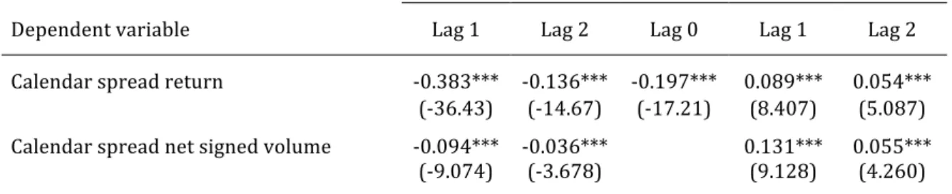
each five-minute interval, we generate calendar spread returns using end-of-interval futures bid-ask midpoint quotes, and we calculate the net signed spread volume for every five-minute interval. Table 6 shows descriptive statistics for the five-minute calendar spread returns and the net signed spread volume. Average five-minute calendar spread return is very close to zero, and the most common slope change is indeed no change
(median equals zero). Slope changes do occur with a standard deviation of more than 20 basis points, and a range between roughly ±200 basis points. Likewise, long delta and short delta calendar spreads are on average balanced during a five-minute period, with a standard deviation of 80 contracts (both futures legs) and a range from -600 to almost +2,000 contracts. Calendar spread returns display negative first order autocorrelation while the corresponding autocorrelation coefficient for net signed volume is positive.
11 Lütkepohl (2005) distinguishes between three different aspects of causality between a set of endogenous variables, instantaneous causality, brief causality, and multi-step causality. Granger (1969) defines the concept of Granger causality, which is based on the notion that one variable is causing another if lagged values of the first variable are helpful for predicting the future outcomes of the other.
18 Both autocorrelation functions decay rather quickly with coefficients beyond the second lag very close to zero.12 [INSERT TABLE 6 HERE] Before running the regressions in the VAR model according to equations (1) and (2), we standardize each variable. Hence, for each variable and day we calculate the mean and
standard deviation of the day’s five-minute observations. Then, we standardize each variable by deducting the mean, and dividing by the standard deviation. Thereby, we control for inter-day variation in volumes and returns. We estimate the regressions with ordinary least squares, using a maximum of two lags in each equation.13
Table 6 holds the results. Both contemporaneous and lagged net signed spread volume affect calendar spread returns. The lagged effects of the first and second order from signed spread volume on calendar spread returns are significantly positive, and suggestive of carrying information. However, the contemporaneous effect is significantly negative, which is not consistent with the story that calendar spread trades contain information relevant for the slope of the volatility term structure. In addition, calendar spread returns exhibit significantly negative autocorrelation of the first and second order. This is in line with an idea that the slope of the volatility term structure tends to revert to, perhaps, a normal case as in Figure 1, after a divergence in the form of either a positive or a negative spread return.
In the equation for net signed calendar spread volume, we find significantly negative
coefficients for lagged spread returns, both on the first and the second lag. These results 12 Each autocorrelation coefficient at lag one and lag two is significantly different from zero at the 1% level. We do not display the test results, but they are available upon request. 13 Each regression shows no significant remaining autocorrelation in the residuals. We do not display the test results, but they are available upon request.
19 imply that returns are causing volume, and are in line with the notion that spread traders use calendar spreads to speculate on future movements in the volatility term structure based on recent corresponding movements. Specifically, lagged positive calendar spread returns lead traders to demand more short delta spreads relative to long delta spreads.
To gauge the economic significance of the results, we re-estimate the VAR model
according to equations (1) and (2) without standardizing the variables.14 The estimation results from the re-estimation form the basis for an impulse-response analysis of how shocks to the dependent variables affect the system. First, we engineer a shock to the volatility term structure slope equal to a 40 basis point calendar spread return during a
five-minute period (period 1 in the following), which corresponds to roughly two standard deviations according to the results in Table 6. To put the 40 basis points in an economic context, we consider the volatility term structure in Figure 1. Suppose that the VXH3 futures price increases with one tick (0.05 index points) from 12.825 to 12.875, while the VXJ3 futures price remains unchanged at 14.725. In this case, the calendar
spread return is the difference in log-returns, which equals 0.39% or about 40 basis points. Hence, the 40 basis point shock roughly corresponds to a one-tick price increase.
[INSERT FIGURE 3 HERE]
Figure 3 displays the results from the impulse response analysis of the calendar spread return shock in period 1. Following the 40 basis point return shock, the VAR model generates a negative calendar spread return of almost 13 basis points, and a negative net
signed calendar spread volume of about ten contracts, in period 2. Then, from period 3
14 The results from the estimation of the VAR model using un-standardized variables exhibit similar coefficient signs and significance as the ones presented in Table 6, and are available from the authors upon request. We believe that it easier to interpret the analysis of economic significance in the un-standardized setting.
20
and onwards, the effect from the shock levels off, and subsequent returns and signed
volumes are indistinguishable from zero. The reaction of the calendar spread return to its own shock comes from the negative first order return autocorrelation. The effect on net signed calendar spread volume is in line with the story that spread traders observe the spread return shock in period 1, and, as a result, trade more short delta calendar spreads
than long delta ones during period 2. As a measure of the total effect from the return shock, the cumulative net signed volume over periods 2 through 10 equals about -12 contracts.
The second shock we bring about is a net signed calendar spread volume equal to 80
contracts (equal to the standard deviation of the variable, reported in Table 6) in period 1. Hence, during this five-minute period the long delta calendar spread volume exceeds the corresponding short delta volume with 80 contracts. Figure 4 illustrates the effects from the volume shock on the calendar spread returns and the net signed spread volume. The immediate effect of the shock is a negative calendar spread return of about 4.5 basis
points during period 1, which follows from the negative contemporaneous correlation (captured by the coefficient 01) between net signed volume and spread return in the VAR model. Subsequent periods see continued positive net calendar spread return at a decreasing rate. In particular, the calendar spread return is positive at 2.8 basis points in period 2, and virtually zero from period 3 and onwards. In total, the volume shock causes a negative cumulative calendar spread return of less than one basis point over subsequent fifty minutes. This effect is clearly at odds with the hypothesis that spread trades contains information. 6. How profitable are calendar spreads?
21
A calendar spread is a bet on the change in the slope of the volatility term structure.
Accordingly, a trader who initiates a long delta calendar spread, i.e., simultaneously buys a short-term futures contract and sells a long-term futures contract, benefits from a future flatter slope, which means that the short-term futures price increases relative to the long-term futures price. With an opposite strategy, a short delta calendar spread will generate
a profit if the slope of the volatility term structure becomes steeper in the future. We consider measures of profitability both within the trading day and until the end-of-day settlement of the futures contracts.
Unfortunately, we are only observing the spread trades, so we have no way of knowing
whether each spread trade initiates a new position or closes an already existing one. Hence, we cannot measure actual realized profits of the calendar spreads. However, as is argued by Fahlenbrach and Sandås (2010), who face similar limitations in their analyses of profitability of option strategies, we can get a sense of the profitability of the calendar spread trades by looking at the profits over different assumed holding periods. The profitability of a calendar spread depends crucially on the associated trading costs. This is true irrespective of which holding period the calendar spread has, and whether a calendar spread trade is initiating or closing a position. We measure trading costs for each futures leg in the spread trade with the effective spread. We observe the effective spread in association with each trade and express it in basis points relative the prevailing futures midpoint in the order book for corresponding regular futures trades at the time of the trade. Trading costs for the calendar spread is the sum of the cost of each leg.
The effective spread for a futures leg is the signed difference between the futures transaction price and the prevailing quoted bid-ask spread midpoint. Denoting the midpoint 6", we define the effective spread 78" for a transaction t as:
22
78" = 9"(:"− 6")/6" (3)
where :" is the futures transaction price and 9" is the direction of trade indicator, defined in line with Harris (1989) relative to the midpoint as 9"= sign(:"− 6"). Hence, 9" = +1 when the transaction is buyer-initiated and 9" = −1 when it is seller-initiated.
[INSERT TABLE 8 HERE]
Table 8 holds the average volume-weighted effective spread for all calendar spreads, and for long delta and short delta strategies respectively. Panel A presents the average effective spread in basis points, while Panel B presents the corresponding average dollar spread. The average value-weighted effective spread is slightly larger than 15 basis
points, with long (short) delta spreads having an effective spread of 16 (14.5) basis points.15 As a comparison, the corresponding average effective spread for regular futures trades is about 16 basis points for the nearby contract and 15 basis points for the second nearby contract over the sample period. Hence, a calendar spread initiated with regular futures would cost more than 30 basis points, which is twice as much as the cost of using the spread trade facility. How much is 15 basis points? Panel B of Table 8 shows a volume-weighted cost of $93.51 for the average nearby calendar spread in our sample. Long delta spreads are more expensive at $97.45 than short delta spreads at $89.70.
We consider a short-term measure of profitability as the five-minute holding period return from the time of each calendar spread trade. Consider a calendar spread at time t,
15 A t-test rejects the null hypothesis of equality between the volume-weighted effective spread for long delta and short delta spreads at the 1% significance level. We do not report the test results, but they are available upon request.
23
containing nearby and second nearby contracts. The five-minute profitability measure
<=" for this strategy is: <=" = 5"[(6"?@ABC% − : "%)/6"%− (6"?@ABC' − :"')/6"'] (4) where 6"?@ABC% (6 "?@ABC ' ) is the futures midpoint price for the nearby (second nearby) contract at time * + 5 minutes, :"% (: "') is the nearby (second nearby) futures transaction price in the spread trade at time t, and the indicator function 5" equals +1 if the calendar spread is long delta, and −1 if it is short delta. We normalize the profitability measure with each respective midpoint 6"% and 6 " ' at the time of recording the spread trade, and express it in basis points. We interpret the measure as the relative change in value of the spread trade position, from the time of the spread trade until five minutes later, with the respective midpoint as the proxy for each futures leg's value.16 According to the results in Table 8, on average, the calendar spreads show a significant five-minute loss of 2.56 basis points ($15.52). Long delta spreads incur a larger loss per trade than short delta spreads. In addition. These numbers seem discouraging for the calendar spread traders, in particular since the average five-minutes slope change
reported in Table 6 (which is similar to our five-minute profit measure) is indistinguishable from zero. Moreover, the spread trades cost on average 15 basis points, or just below $100, to initiate. To consider the costs, we calculate the net dollar profit for each calendar spread trade by deducting the effective spread from the five-minute profit. Figure 5 displays the distribution function for the net five-minute profits. With this measure, about 77% of both the long delta and the short delta calendar spreads are not
16 We evaluate the calendar spreads initiated with less than five minutes left until the closing time using the daily settlement prices as for the mark-to-market profit measure in equation (4).
24
profitable, while the remaining 23% exhibit returns in excess of initiation transaction
costs. [INSERT FIGURE 5 HERE] As a measure of profitability until the end of the trading day, we consider the mark-to-market gains and losses of the spread trades relative to the day-end futures settlement prices. The mark-to-market profitability measure ==",N for a calendar spread at time t on day s, containing nearby and second nearby contracts, is: ==",N= 5"[(:NO",N% − : ",N%)/6",N% − (:NO",N' − :",N')/6",N' ] (4) where :NO",N% (: NO",N' ) is the settlement price for nearby (second nearby) contract on day s, and :",N% (:",N') is the nearby (second nearby) futures transaction price in the spread trade at time t on day s. The results in Table 8 show an average profit across all calendar spreads equal to 2.07 basis points ($9.01). Hiding behind this significantly positive profit is a significantly negative profit of 4.40 basis points ($46.70) for long delta spreads and a significantly positive profit of 8.30 basis points ($62.64) for short delta spreads. The short delta calendar spread trades are more successful than the corresponding long delta spreads,
given that they settle at the end of the trading day. In Figure 6, we note that 70% of the long delta spread trades have a negative profit, net of transactions costs, while the corresponding number for short delta spreads is only 43%. Hence, a majority of the short delta calendar spreads earn returns in excess of transactions costs if closed towards the end of the trading day.
25 7. Concluding remarks A VIX futures calendar spread involves buying/selling a futures contract maturing in one month and selling/buying another one maturing in a different month. Although futures calendar spreads are popular among traders in the VIX futures market, no existing studies investigate these trading spread strategies. In this paper, we identify actual VIX futures spread strategies from data and investigate if information or speculation drives trading in VIX futures calendar spreads. In doing so, we argue that a calendar spread trade is a bet on the change in the slope of the volatility term structure. We also examine the profitability of VIX futures calendar spreads.
VIX futures calendar spreads represent a daily turnover in excess of 500 million dollars, which corresponds to about 20% of daily total VIX futures trading volume. We find that speculation rather than information about changes in the slope of the volatility term structure is driving calendar spread trades. On average, a calendar spread costs a little less than $100 (about 15 basis points). If settled at the end of the trading day, 43% of the
26
References
Bakshi, G., & Madan, D. (2000). Spanning and derivative-security valuation. Journal of Financial Economics, 55, 205-238. Black, F., & Scholes, M. (1973). The pricing of options and corporate liabilities. Journal of Political Economy, 81, 637-654. Breeden, D., & Litzenberger, R. (1978). Prices of state-contingent claims implicit in option prices, Journal of Business, 621-651. Chan, K., Chung, Y. P., & Fong, W. M. (2002). The informational role of stock and option volume. Review of Financial Studies, 15, 1049-1075.
Chaput, J., & Ederington, L. (2003). Option spread and combination trading. Journal of Derivatives, 10, 72-88. Chaput, J., & Ederington, L. (2005). Volatility trade design. Journal of Futures Markets, 25, 243-279. Chaput, J., & Ederington, L. (2008). Ratio spreads. Journal of Derivatives, 15, 41-57. Cox, J., & Ross, S. (1976). The valuation of options for alternative stochastic processes. Journal of Financial Economics, 3, 145-166. Egloff, D., Leippold, M., & Wu, L. (2010). The term structure of variance swap rates and optimal variance swap investments. Journal of Financial and Quantitative Analysis, 45, 1279-1310.
Fahlenbrach, R., & Sandås, P. (2010). Does information drive trading in option strategies?
27
Frino, A., Kruk, J., & Lepone, A. (2007). Transactions in futures markets: Informed or
uninformed? Journal of Futures Markets, 27, 1159-1174.
Frino, A., & McKenzie, M. (2002). The pricing of stock index futures spreads at contract expiration. Journal of Futures Markets, 22, 451-469.
Frino, A., & Oetomo, T. (2005). Slippage in futures markets: Evidence from the Sydney
Futures Exchange. Journal of Futures Markets, 25, 1129-1146.
Granger, C. (1969). Investigating causal relations by econometric models and cross-spectral methods. Econometrica, 37, 424-438.
Harris, L. (1989). A day-end transaction price anomaly. Journal of Financial and Quantitative Analysis, 24, 29-45.
Hasbrouck, J. (1991). Measuring the information content of stock trades. Journal of
Finance, 46, 179-207.
Huskaj, B., & Nordén, L. (2015). Two order books are better than one? Trading At Settlement (TAS) in VIX futures. Journal of Futures Markets, 35, 506-521.
Johnson, T. (2016). Risk premia and the VIX term structure. Journal of Financial and Quantitative Analysis (forthcoming).
Lee, C. & Ready, M. (1991). Inferring trade direction from intraday data. Journal of Finance, 46, 733-747.
Liu, J. & Pan, J. (2003). Dynamic derivative strategies. Journal of Financial Economics, 69, 401–430.
28
Lu, Z., & Zhu, Y. (2010). Volatility components: The term structure dynamics of VIX
futures. Journal of Futures Markets, 30, 230–256 (2010).
Lütkepohl, H. (2005). New introduction to multiple time series analysis. Berlin: Springer Verlag.
Newey, W., & West, K. (1987). A simple, positive semi-definite, heteroskedasticity and
autocorrelation consistent covariance matrix. Econometrica, 55, 703–708. Newey, W., & West, K. (1994). Automatic lag selection in covariance matrix estimation. Review of Economic Studies, 61, 631–653. Ross, S. (1976). Options and efficiency. Quarterly Journal of Economics, 90, 75-89. Stoll, H. (2000). Friction. Journal of Finance, 55, 1479-1514. Tsai, W. C., Chiu, Y. T., and Wang, Y. H. (2015). The information content of trading activity and quote changes: Evidence from VIX options. Journal of Futures Markets, 35, 715-737.
29
#RIC Date[L] Time[L] Price Volume Seq. No. Qualifiers VXU3 14-mar-13 09:28:46.847269 18.45 1 164098 VXH3 14-mar-13 09:28:59.407704 12.80 1 164256 VXM3 14-mar-13 09:29:00.296596 16.65 6 164600 VXN3 14-mar-13 09:29:00.283709 17.40 4 164601 VXM3 14-mar-13 09:29:02.912865 16.65 1 164857 VXM3 14-mar-13 09:29:02.912865 16.65 2 164858 VXM3 14-mar-13 09:29:02.912865 16.65 1 164859 VXM3 14-mar-13 09:29:02.912865 16.65 2 164860 VXM3 14-mar-13 09:29:02.912865 16.65 1 164861 VXH3 14-mar-13 09:29:07.347090 12.83 1 164931 SPR[PRC_QL2] VXJ3 14-mar-13 09:29:07.343232 14.72 1 164932 SPR[PRC_QL2] VXK3 14-mar-13 09:29:08.136156 15.85 40 165001 VXK3 14-mar-13 09:29:19.029513 15.85 3 165241 VXJ3 14-mar-13 09:29:20.697628 14.72 3 165296 SPR[PRC_QL2] VXK3 14-mar-13 09:29:20.693528 15.83 3 165297 SPR[PRC_QL2] Table 1: Output from the TRTH database for a sequence of VIX futures trades just before 9:30 AM on March 14, 2013. #RIC denotes the futures contract (maturity), Date[L] is the local (CST) date, Time[L] is the local time (CST) with accuracy down to microsecond, Price is trade price, Volume is the number of contracts traded, Seq. No. is the sequence number of trades, and Qualifier denotes type of trade, where SPR[PRC_QL2] indicates a spread trade.
30
Trading Volume (contracts) Trading Volume (million $) Number of Transactions Contract
Maturity Regular Trades % Spread Trades % Regular Trades % Spread Trades % Regular Trades % Spread Trades % All 106,106 68.73 48,267 31.27 1,742 68.16 814 31.84 15,064 54.69 12,479 45.31 1st 49,946 80.45 12,141 19.55 781 80.61 188 19.39 6,377 67.60 3,056 32.40 2nd 30,668 66.58 15,392 33.42 505 66.56 253 33.44 4,275 53.00 3,790 47.00 3rd 11,205 57.28 8,358 42.72 194 57.30 144 42.70 1,520 43.75 1,954 56.25 4th 6,112 53.88 5,232 46.12 109 53.90 94 46.10 1,052 43.68 1,356 56.32 5th 4,163 54.82 3,431 45.18 77 54.80 63 45.20 833 45.35 1,004 54.65 6th 2,476 53.58 2,145 46.42 47 53.52 41 46.48 579 44.85 713 55.15 7th 1,260 51.74 1,175 48.26 24 51.66 23 48.34 325 42.60 438 57.40 8th 225 40.94 324 59.06 4 40.82 6 59.18 84 37.92 138 62.08 9th 51 42.38 70 57.62 1 42.22 1 57.78 20 39.22 31 60.78 Table 2: Average daily trading volume (the number of traded futures contracts and millions of dollars) and number of transactions for regular trades and spread trades in VIX futures. Averages are for all contracts (All) and each maturity, from the nearby contract (1st) to the deferred contracts (2nd through 9th). Sample period is March 14, 2013 to October 25, 2013 (157 full trading days).
31 Contract 1st 2nd 3rd 4th 5th 6th 7th 8th 9th 1st 1,796 184 86 55 28 20 1 0 2nd 13,979 697 102 64 30 17 2 0 3rd 1,537 6,163 418 65 25 12 2 0 4th 648 709 3,469 270 44 25 3 1 5th 444 455 374 1,948 202 27 6 1 6th 187 197 146 259 1,246 139 9 1 7th 102 95 57 115 143 744 46 2 8th 5 10 7 9 25 36 225 11 9th 0 3 0 6 4 5 7 49 Table 3: The lower triangular part of the table presents average daily trading volume (the number of traded futures contracts), and the upper triangular part holds average daily number of transactions, for calendar spread strategies in VIX futures. Strategies involve a position in a row-wise contract together with a column-wise contract, one long and the other one short. Averages are for each pair of contract maturities, involving the nearby contract (1st) and the deferred contracts (2nd nearby through 9th). Sample period is March 14, 2013 to October 25, 2013 (157 full trading days).
32 Strategy All 1st/2nd 2nd/3rd 3rd/4th Panel A: Average daily number of calendar spread transactions Calendar spread 4,394 1,796 697 418 (40.86) (15.87) (9.51) Long delta 2,168 881 361 205 (49.35) (49.05) (51.72) (49.07) Short delta 2,226 915 337 213 (50.65) (50.95) (48.28) (50.93) Panel B: Average daily calendar spread trading volume Calendar spread 33,409 13,979 6,163 3,469 (41.84) (18.45) (10.38) Long delta 16,811 7,020 3,210 1,680 (50.32) (50.22) (52.08) (48.44) Short delta 16,598 6,959 2,953 1,788 (49.68) (49.78) (47.92) (51.56) Table 4: Average daily number of transactions (Panel A) and average daily trading volume (the number of traded futures contracts, Panel B) for calendar spread strategies in VIX futures. The strategy “Calendar spread” is a matched pair of two futures contracts, one long and the other one short. “Long delta” is a calendar spread with a long position in the futures contract with short maturity and a short position in the contract with long maturity. “Short delta” is a calendar spread with a short position in the futures contract with short maturity and a long position in the contract with long maturity. We also obtain averages for calendar spreads for specific pairs of contract maturities; involving the nearby and second nearby contracts (1st/2nd), second nearby and third nearby contracts (2nd/3rd), and third nearby and fourth nearby contracts (2nd/3rd). Sample period is March 14, 2013 to October 25, 2013 (157 full trading days).
33
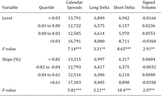
Variable Quartile Calendar Spreads Long Delta Short Delta Volume Signed Level <-0.03 13,791 6,849 6,942 -0.0166 -0.03 to 0.00 12,732 6,575 6,157 0.0236 0.00 to 0.03 12,585 6,614 5,970 0.0553 >0.03 16,791 8,080 8,711 -0.0360 F-value 7.14*** 3.31** 8.65*** 2.91** Slope (%) <-0.82 13,315 6,997 6,317 0.0604 -0.82 to -0.04 12,793 6,417 6,375 -0.0032 -0.04 to 0.61 12,516 6,306 6,210 0.0040 >0.61 17,303 8,405 8,898 -0.0358 F-value 5.81*** 3.21** 10.4*** 2.97**
Table 5: Quartile average daily trading volume (the number of traded futures contracts) for calendar spreads in nearby (1st) and second nearby (2nd) VIX futures. Averages are for quartiles of the Level (VIX return) and Slope (difference between nearby futures return and second nearby futures contract return). Each return is the difference between the logarithm of day-end index prices and futures settlement prices respectively. Long (short) delta denotes a strategy that takes a long (short) position in the nearby futures contract and a short (long) position in second nearby contract. Signed volume is the daily average relative difference between long delta volume and short delta volume. Sample period is March 14, 2013 to October 25, 2013 (157 full trading days). Each F-value results from an ANOVA test of equality across quartiles, where standard errors are using the Newey and West (1987, 1994) HAC covariance matrix. *, **, *** indicate statistical significance at the 10%, 5%, and 1%, respectively.
34
Statistic Return Volume Signed
Mean 0.0033 0.2578 Median 0.0000 0.0000 Maximum 229.62 1,950 Minimum -227.64 -606 St. Dev. 22.640 80.460 Autocorrelation Lag 1 -0.273 0.129 Lag 2 -0.008 0.058 Lag 3 0.014 0.031 Table 6: Descriptive statistics for five-minute nearby VIX futures calendar spread returns (Return) and five-minute net signed volume (Signed Volume) from calendar spread trade strategies combining nearby and second nearby VIX futures. Each calendar spread return equals the difference between nearby futures return and second nearby futures return, expressed in basis points. The net signed spread volume is the difference between the long delta and short delta calendar spread volume, where long (short) delta denotes a strategy that takes a long (short) position in the nearby futures contract and a short (long) position in second nearby contract. Sample period is March 14, 2013 to October 25, 2013 (157 full trading days).
35
Explanatory variables
Lagged spread returns Lagged spread net signed volume Dependent variable Lag 1 Lag 2 Lag 0 Lag 1 Lag 2 Calendar spread return -0.383*** -0.136*** -0.197*** 0.089*** 0.054***
(-36.43) (-14.67) (-17.21) (8.407) (5.087)
Calendar spread net signed volume -0.094*** -0.036*** 0.131*** 0.055***
(-9.074) (-3.678) (9.128) (4.260)
Table 7: Regression analysis of the relationship between standardized five-minute nearby VIX futures calendar spread returns and standardized five-minute net signed volume from calendar spread trade strategies combining nearby and second nearby VIX futures. We estimate the following VAR model:
!"= $%!"&%+ $(!"&(+ )*+"+ )%+"&%+ )(+"&(+ ,%," +"= .%!"&%+ .(!"&(+ /%+"&%+ /(+"&(+ ,(,"
where !"= (!"%− !
"() is the calendar spread return (change in slope), measured as the change in futures
midpoint quotes, !"% is the nearby futures return, and !"( is the return of the second nearby futures contract
at time t. +" is the net signed spread volume, i.e., the difference between the long delta and short delta
calendar spread volume, between time 3 − 1 and time t. The a's, b's, c's, and d's are coefficients, while ,%,"
and ,(," are residual terms. We standardize each return and net signed volume by subtracting each variable's mean and dividing by the standard deviation of the day. Sample period is March 14, 2013 to October 25, 2013 (157 full trading days). t-values are in parentheses. *, **, *** indicate statistical significance at the 10%, 5%, and 1%, respectively. Standard errors are using the Newey and West (1987, 1994) HAC covariance matrix.
36
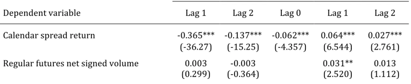
Explanatory variables
Lagged spread returns Lagged regular net signed volume Dependent variable Lag 1 Lag 2 Lag 0 Lag 1 Lag 2 Calendar spread return -0.365*** -0.137*** -0.062*** 0.064*** 0.027***
(-36.27) (-15.25) (-4.357) (6.544) (2.761)
Regular futures net signed volume 0.003 -0.003 0.031** 0.013
(0.299) (-0.364) (2.520) (1.112)
Table 7b: Regression analysis of the relationship between standardized five-minute nearby VIX futures calendar spread returns and standardized five-minute net signed volume from regular futures trades combining nearby and second nearby VIX futures. We estimate the following VAR model:
!"= $%!"&%+ $(!"&(+ )*+"+ )%+"&%+ )(+"&(+ ,%," +"= .%!"&%+ .(!"&(+ /%+"&%+ /(+"&(+ ,(,"
where !"= (!"%− !
"() is the calendar spread return (change in slope), measured as the change in futures
midpoint quotes, where !"% is the nearby futures return and !"( is the return of the second nearby futures
contract at time t, +" is the net signed futures volume, i.e., the difference between long delta and short delta
spread volume, from fictive spread trade strategies formed with regular futures contracts, between time 3 − 1 and time t, the a's, b's, c's, and d's are coefficients, while ,%," and ,(," are residual terms. We standardize
each return and net signed volume by subtracting each variable's mean and dividing by the standard deviation of the day. Sample period is March 14, 2013 to October 25, 2013 (157 full trading days). t-values are in parentheses. *, **, *** indicate statistical significance at the 10%, 5%, and 1%, respectively. Standard errors are using the Newey and West (1987, 1994) HAC covariance matrix.
37
Strategy Number of
observations Effective spread 5-minutes Settlement Panel A: Average volume-weighted per trade profit (basis points) All calendar spreads 281,895 15.26 -2.56*** 2.07*** (-20.7) (3.32) Long delta 143,616 16.03 -3.67*** -4.40*** (-20.3) (-4.61) Short delta 138,279 14.52 -1.45*** 8.30*** (-8.55) (10.3) Panel B: Average volume-weighted per trade profit (dollars) All calendar spreads 281,895 93.51 -15.52 9.01 Long delta 143,616 97.45 -21.46 -46.70 Short delta 138,279 89.70 -9.80 62.64 Table 8: Average volume-weighted profitability of VIX futures calendar spreads in nearby (1st) and second nearby (2nd) VIX futures. Long (short) delta denotes a strategy that takes a long (short) position in the nearby futures contract and a short (long) position in second nearby contract. We obtain the effective spread for each nearby and second nearby futures contract respectively, as the signed relative difference between each futures transaction price and the prevailing quoted bid-ask spread midpoint, and then summed together for the calendar spread. The five-minute (5-minute) profitability measure 56" is:
56"= /"[(8"9:;<=% − >
"%)/8"%− (8"9:;<=( − >"()/8"(]
where 8"9:;<=% (8"9:;<=( ) is the futures midpoint price for the nearby (second nearby) contract at time 3 +
5 minutes, >"% (>"() is the nearby (second nearby) futures transaction price in the spread trade at time t, and
the indicator function /" equals +1 if the calendar spread is long delta, and −1 if it is short delta. We
normalize the profitability measure with each respective midpoint 8"% and 8"( at the time the spread trade
is recorded, and expressed in basis points. The mark-to-market (Settlement) profitability measure 66",B
for a calendar spread at time t on day s is:
66",B= /"[(>BC",B% − >",B%)/8%",B− (>BC",B( − >",B()/8",B( ]
where >BC",B% (>BC",B( ) is the settlement price for nearby (second nearby) contract on day s, and >",B% (>",B() is the
nearby (second nearby) futures transaction price in the spread trade at time t on day s. *, **, *** indicate significantly different from zero according to a t-test at the 10%, 5%, and 1%, respectively. Sample period is March 14, 2013 to October 25, 2013 (157 full trading days).
38 Principal Component Contract Maturity 1 2 3 Eigenvectors 1st -0.312 0.667 0.507 2nd -0.331 0.423 -0.155 3rd -0.337 0.153 -0.456 4th -0.340 0.059 -0.297 5th -0.340 -0.087 -0.235 6th -0.336 -0.274 -0.150 7th -0.336 -0.301 0.033 8th -0.335 -0.299 0.292 9th -0.331 -0.293 0.510 Eigenvalue (%) 94.02 3.71 0.81 Appendix A: Principal component analysis of VIX futures (log) returns. Each return series is obtained on a daily basis, using daily futures settlement prices, for each maturity, from the nearby contract (1st) to the deferred contracts (2nd nearby through 9th). Sample period is March 14, 2013 to October 25, 2013 (157 full trading days). Our interpretation of the principal components is in line with Lu and Zhu (2010). The first principal component has almost identical loadings on all nine maturities. Thus, the first component is the level of the VIX futures term structure. The second component has positive loadings on the four shortest maturities and negative loadings on the five longest maturities. Therefore, we interpret the second component as the slope of the term structure. Finally, the third component has a positive loading on the nearby maturity, negative loadings on the second through sixth maturities, and positive loadings on the seventh through ninth maturities. This pattern of the loadings is consistent with a curvature interpretation of the third component.
39 Figure 1: The midpoint between the bid quote and the ask quote prevailing in the order book for each VIX futures contract just before 9:30 am on March 14, 2013. On this date, VXH3 is the nearby contract with maturity in March 2013, while VXJ3, VXK3, ..., VXX3 are deferred contracts with maturity in April, May, ..., November 2013. 12.825 14.725 15.875 16.675 17.375 17.925 18.425 18.825 19.125 10.0 15.0 20.0 VXH3 VXJ3 VXK3 VXM3 VXN3 VXQ3 VXU3 VXV3 VXX3 Fu tu re s pr ic e (m id po in t) Futures contract
40 Figure 2: Average trading volume (the number of traded futures contracts, left-hand axis), and cumulative average trading volume (right-hand axis), for calendar spreads in nearby (1st) and second nearby (2nd) VIX futures during five-minute intraday periods. Long (short) delta denotes a strategy that takes a long (short) position in the nearby futures contract and a short (long) position in second nearby contract. Sample period is March 14, 2013 to October 25, 2013 (157 full trading days). 0 1000 2000 3000 4000 5000 6000 7000 0 200 400 600 800 1000 1200 1400 07: 00 07: 15 07: 30 07: 45 08: 00 08: 15 08: 30 08: 45 09: 00 09: 15 09: 30 09: 45 10: 00 10: 15 10: 30 10: 45 11: 00 11: 15 11: 30 11: 45 12: 00 12: 15 12: 30 12: 45 13: 00 13: 15 13: 30 13: 45 14: 00 14: 15 14: 30 14: 45 15: 00 15: 15 Cu m ul at iv e tr ad in g vo lu m e Tr ad in g vo lu m e Time of the trading day Long delta Short delta Long delta (cum.) Short delta (cum.)
41 Figure 3: Effects of a period 1 shock in the calendar spread return equal to 40 basis points on calendar spread returns and net signed volume during subsequent five-minute periods. -20 -10 0 10 20 30 40 1 2 3 4 5 6 7 8 9 10 Ca le nd ar sp re ad re tu rn ( bp s) Five-minute period -20 0 20 40 60 80 1 2 3 4 5 6 7 8 9 10 Ca le nd ar sp re ad n et s ig ne d vo lu me (c on tra ct s) Five-minute period
42 Figure 4: Effects of a period 1 shock in the calendar spread net signed volume equal to 160 contracts on net signed volume and calendar spread returns during subsequent five-minute periods. -20 0 20 40 60 80 1 2 3 4 5 6 7 8 9 10 Ca le nd ar sp re ad n et s ig ne d vo lu me (c on tra ct s) Five-minute period -20 -10 0 10 20 30 40 1 2 3 4 5 6 7 8 9 10 Ca le nd ar sp re ad re tu rn ( bp s) Five-minute period