Environmental impact of chemical and mechanical weed control in agriculture : a comparing study using Life Cycle Assessment (LCA) methodology

Full text

(1)SIK-rapport Nr 719 2004. Environmental impact of chemical and mechanical weed control in agriculture - a comparing study using Life Cycle Assessment (LCA) methodology. Serina Ahlgren.

(2)

(3) SIK-rapport Nr 719 2004. Environmental impact of chemical and mechanical weed control in agriculture - a comparing study using Life Cycle Assessment (LCA) methodology. Serina Ahlgren. SR 719 ISBN 91-7290-232-9.

(4)

(5) ABSTRACT In this paper, two farming systems have been compared in a Life Cycle Assessment, LCA. The LCA is a methodology that allows the viewer to analyse a product or a service through its entire life cycle. The Swedish government has formulated 15 environmental goals. Amongst these, it is stated that the amount of chemicals used in agriculture should be minimised. It is therefore of great interest to look at alternative ways of fighting weeds. In this study a farming system with chemical weed control is compared to a farming system with mechanical weed control regarding energy use and environmental impact. The base of comparance, the functional unit, was the total yield from all crops in a determined crop sequence during one year. Data for the chemical scenario was collected from Fäcklinge Fors farm in Tierp, Sweden. Some data were collected from literature in order to give the study a more general validity. The farm in Tierp has a crop sequence that also would be suitable for a farm with mechanical weed control (barley, ley I, ley II, winter wheat, oats, potato). The mechanical scenario was thus a hypothetical switch to a mechanical weed control system at the same site. Most other conditions were the same for the two scenarios, for example fungus and insect control. The yields on the other hand were assumed to differ between the scenarios. Since the functional unit was based on the amount of products, the area of grown land differed between the scenarios. The results indicated that the mechanical scenario had a larger contribution to the impact categories energy, global warming, eutrophication, acidification and photo-oxidant formation. But the differences between the scenarios were small compared to the farming system in total. The study showed that a mechanical weed control system not necessarily cause much larger emissions or energy use, but has the great advantage of not using herbicides. Amongst the crops, oats showed the largest diversion between the chemical and the mechanical scenario. This due to the fact that the heaviest direct weed control, stubble cultivation was done here. The production of mineral fertilisers had the largest contribution to the global warming potential; the weed control had only marginal effect on the results. The nitrate leaching had the largest influence on eutrophication. In the acidification category, field operations were the largest contributor. The field operations were also the largest contributor to photo-oxidant formation. The energy usage in the mechanical scenario was only 4% larger than in the chemical scenario..

(6) SAMMANFATTNING I denna studie jämfördes två odlingssystem i en livscykelanalys (LCA). LCA är en metod där en produkt eller tjänst studeras genom hela sin livscykel. Sveriges riksdag och regering har antagit 15 miljömål för att nå en hållbar utveckling. Bland dessa återfinns en minskad användning av kemikalier i jordbruket. Det är därför intressant att studera alternativa metoder för att bekämpa ogräs. I detta examensarbete har två odlingssystem jämförts, ett med kemisk och ett med mekanisk ogräsbekämpning, med avseende på miljöpåverkan och energianvändning. Basen för jämförelse, den funktionella enheten, var den totala skörden från alla grödor i en växtföljd under ett år. Dataunderlag till det scenariot med kemisk bekämpning hämtades från Fäcklinge Fors gård i Tierp, Sverige. Vissa siffror inhämtades dock från litteratur. Gården i Tierp har en växtföljd som även skulle passa bra för mekanisk ogräsbekämpning (korn, vall I, vall II, höstvete, havre, potatis). Det mekaniska scenariot var alltså en hypotetisk omläggning till mekanisk ogräsbekämpning från dagens system. Alla andra förutsättningar antogs vara de samma, till exempel handelsgödsel, fungicider och insekticider. Skördarna antogs däremot skilja mellan scenarierna. Eftersom den funktionella enheten var baserad på massa, så skiljde sig den odlade arealen åt mellan det kemiska och mekaniska scenariot. Resultaten indikerade att det mekaniska scenariot gav ett högre bidrag till miljöpåverkanskategorierna energi, växthuseffekt, eutrofiering, försurning och fotooxidansbildning. Skillnaden mellan scenarierna var dock små om man jämför med odlingssystemen i sin helhet. Denna studie visade att ett odlingssystem med mekanisk ogräsbekämpning inte nödvändigtvis orsakar mycket större utsläpp eller energianvändning än ett system med kemisk ogräsbekämpning, men har den stora fördelen att inte använda herbicider. Mellan de olika grödorna fanns stora skillnader. Havre visade störst skillnad mellan det kemiska och mekaniska scenariot, vilket beror på de tunga mekaniska insatserna i den grödan, främst stubbebearbetning. Produktionen av handelsgödsel bidrog mest till växthuseffekten medan ogräsbekämpningen hade marginell påverkan. Utlakningen resulterade i det största bidraget till övergödningen. Till försurning bidrog operationer på fält mest. Fältoperationer var även den största bidragande faktorn till fotooxidansbildningen. Energianvändningen var endast 4 % högre i det mekaniska scenariot jämfört med det kemiska..

(7) FOREWORD This project was conducted as a Master’s Thesis at the department of agricultural engineering at the Swedish University of Agricultural Science (SLU). The initiator of the project was the Swedish Institute for Food and Biotechnology (SIK) in Gothenburg, Sweden. SIK and SLU are involved in the program Sustainable Food Production, FOOD 21 (in Swedish: MAT 21). The overall long-term goal of the FOOD 21 program is to define optimal conditions for sustainable food production that generate high quality food products. This paper forms a part of the MAT 21 program. I would very much like to thank Berit Mattsson (SIK), Per-Anders Hansson (SLU) and Maria Wivstad (SLU) for their supervision and guidance throughout the project. I would also like to thank Hans Fredriksson for answering all of my questions. Finally, I would like to thank my husband and children for their patience and support at all times during this project..

(8)

(9) TABLE OF CONTENTS. 1 INTRODUCTION................................................................................................................... 3 1.1 Goal and scope ..............................................................................................................................................3. 2 WHAT IS A LIFE CYCLE ASSESSMENT?......................................................................... 4 2.1 Methodology .................................................................................................................................................4 2.2 System Boundaries ........................................................................................................................................4 2.3 Functional unit...............................................................................................................................................5 2.4 Allocation ......................................................................................................................................................5 2.5 Impact assessment .........................................................................................................................................6. 3 DEFINITION OF THIS LCA ................................................................................................. 7 3.2 Setting up the scenarios.................................................................................................................................7 3.3 System boundaries.........................................................................................................................................8 3.4 Functional unit...............................................................................................................................................8 3.5 Impact categories...........................................................................................................................................8 3.5.1 Resources...............................................................................................................................................8 3.5.2 Global warming.....................................................................................................................................9 3.5.3 Eutrophication.......................................................................................................................................9 3.5.4 Acidification ..........................................................................................................................................9 3.5.5 Photo-oxidant formation........................................................................................................................9 3.5.6 Pesticides.............................................................................................................................................10. 4 FARMING SYSTEMS ......................................................................................................... 11 4.1 Crop sequence .............................................................................................................................................11 4.1.1 Literature.............................................................................................................................................11 4.1.2 Chosen crop sequence .........................................................................................................................13 4.2 Presentation of Fäcklinge Fors Farm...........................................................................................................13 4.3 Yields ..........................................................................................................................................................13 4.3.1 Fäcklinge Fors.....................................................................................................................................13 4.3.2 Literature.............................................................................................................................................13 4.3.3 Chosen yields.......................................................................................................................................15 4.4 Fertilisers.....................................................................................................................................................15 4.4.1 Fäcklinge Fors.....................................................................................................................................15 4.4.2 Literature.............................................................................................................................................16 4.2.3 Chosen fertilisers.................................................................................................................................16 4.5 Seed .............................................................................................................................................................17 4.5.1 Fäcklinge Fors.....................................................................................................................................17 4.5.2 Literature.............................................................................................................................................17 4.5.3 Chosen amount of seed ........................................................................................................................17 4.6 Tillage operations ........................................................................................................................................18 4.6.1 Literature.............................................................................................................................................18 4.7 Pesticides.....................................................................................................................................................18 4.7.1 Fäcklinge Fors.....................................................................................................................................18 4.7.2 Literature.............................................................................................................................................18 4.7.3 Chosen pesticides ................................................................................................................................19 4.8 Chemical weed control................................................................................................................................19 4.8.1 Fäcklinge Fors.....................................................................................................................................19 4.8.2 Literature.............................................................................................................................................19 4.8.3 Chosen chemical weed control ............................................................................................................20 4.9 Mechanical weed control.............................................................................................................................20 4.9.1 Literature.............................................................................................................................................20 4.9.2 Chosen mechanical weed control ........................................................................................................21 4.10 Summary of chosen farming systems........................................................................................................21. 1.

(10) 5 INVENTORY OF FARMING SYSTEMS ........................................................................... 24 5.1 Field operations ...........................................................................................................................................24 5.2 Diesel production ........................................................................................................................................24 5.3 Electricity production ..................................................................................................................................24 5.5 Pesticide and herbicide production..............................................................................................................24 5.4 Mineral fertiliser production........................................................................................................................25 5.6 Seed production...........................................................................................................................................25 5.7 Production of stretch film............................................................................................................................25 5.8 Emissions of N in cropping .........................................................................................................................25 5.8.1 Nitrate (NO3-N) ...................................................................................................................................25 5.8.2 Ammonia (NH3) ...................................................................................................................................26 5.8.3 Nitrous oxide (N2O) .............................................................................................................................26 5.9 Losses of phosphorus ..................................................................................................................................27. 6 IMPACT ASSESSMENT ..................................................................................................... 27 6.1 Energy .........................................................................................................................................................27 6.2 Global Warming ..........................................................................................................................................29 6.3 Eutrophication .............................................................................................................................................31 6.4 Acidification................................................................................................................................................32 6.5 Photo-oxidant formation..............................................................................................................................33 6.6 Pesticide use ................................................................................................................................................34. 7 DISCUSSION ....................................................................................................................... 34 7.1 Sensitivity analysis ......................................................................................................................................35 7.1.1 Yields ...................................................................................................................................................35 7.1.2 Mechanical weed control.....................................................................................................................35 7.2 Pesticides in the environment......................................................................................................................36 7.3 Long term effects of weeds in a mechanical weed control system..............................................................36 7.3 Humus content.............................................................................................................................................38 7.4 Machinery....................................................................................................................................................38. 8 REFERENCES...................................................................................................................... 39 8.1 Literature .....................................................................................................................................................39 8.2 Personal communication .............................................................................................................................42 8.3 Internet ........................................................................................................................................................42. APPENDIX 1. CHARACTERISATION FACTORS.............................................................. 43 APPENDIX 2. EXHAUST EMISSIONS FROM FIELD OPERATIONS.............................. 44 APPENDIX 3. PRODUCTION OF DIESEL AND ELECTRICITY ...................................... 45 APPENDIX 4. PRODUCTION OF PESTICIDES .................................................................. 46 APPENDIX 5. PRODUCTION AND TRANSPORT OF MINERAL FERTILISER............. 47 APPENDIX 6. PRODUCTION OF STRETCH FILM............................................................ 48 APPENDIX 7. BARLEY CHEMICAL SCENARIO .............................................................. 47 APPENDIX 8. BARLEY MECJANICAL SCENARIO.......................................................... 48 APPENDIX 9. LEY I CHEMICAL AND MECHANICAL SCENARIO............................... 49 APPENDIX.10. LEY II CHEMICAL SCENARIO................................................................. 50 APPENDIX 11. LEY II MECHANCIAL SCENARIO ........................................................... 51 APPENDIX 12. WINTER WHEAT CHEMICAL SCENARIO ............................................. 52 APPENDIX 13. WINTER WHEAT MECHANCIAL SCENARIO ....................................... 53 APPENDIX 14. OATS CHEMICAL SCENARIO.................................................................. 54 APPENDIX 15. OATS MECHANICAL SCENARIO ............................................................ 55 APPENDIX 16. POTATO CHEMICAL SCENARIO ............................................................ 56 APPENDIX 17. POTATO MECHANCIAL SCENARIO....................................................... 57. 2.

(11) 1 INTRODUCTION Weeds have always been a problem in cultivation. More specifically weeds lower the yields and the quality of the yield. Weeds can also be carriers of infections, fungus and other diseases, which can contaminate the crops. Large number of weeds can also cause cereal to lodge. Weeds can also be positive, for such things as biodiversity. Increasing the number of species and attracting wild animal can be a high priority. In this paper, though, weeds are something we want to minimise. The weeds have to be regulated, not causing harvest decrease or other problems. There are in principal two ways of fighting weeds; direct and indirect. Direct means taking action against the weeds for example by ploughing, hoeing, harrowing, hand plucking, flame treatment and by spraying herbicides. Indirect weed control can for example be a wellplanned crop sequence. It also includes choosing crops that are competitive and to use clean seed. Taking technical cropping measures, such as delayed sowing, increasing or decreasing row distance and adjusting the amount of seed are other examples of indirect weed control (Fogelfors, 1995). Up to World War II a lot of effort was put into indirect weed control, since weeds were a limiting factor for the yield. Then something changed; the herbicides were introduced. This made it possible to have a non-diversified crop sequence without any weed problems. But the negative effects of this type of farming systems have proven to be many. Not only is it dangerous for the farmers to handle the chemicals, but it is also damaging for the environment. It affects biodiversity in a negative way and can give rise to new compositions of species. Traces of herbicides are also found in harvested crops and ground- and surface waters (Fogelfors, 1995; Gummesson, 1992). The Swedish government has formulated an environmental policy. In this policy, that contains 15 goals, it is among other things stated that by the year 2005 twenty percent of arable land should be organically farmed (Miljömålsportalen, www). In organic farming herbicides are not allowed. In the environmental goals it is also stated that the usage of chemicals shall be minimised in order to maintain a non-toxic environment. It is therefore of great interest to investigate alternative ways of fighting weeds, such as mechanical weed control. But what impact does a mechanical weed control system have on the environment? This is the main question in this paper. Weed control is only a part of the whole farming system. Whatever conclusions made in this paper, it does not determine whether one system or the other is more suitable. What effect agriculture has on the environment depends on a number of factors all woven together in a complicated pattern.. 1.1 Goal and scope My objective is to study the difference between a farming system with chemical weed control and a farming system with mechanical weed control in a life cycle assessment (LCA).. 3.

(12) 2 WHAT IS A LIFE CYCLE ASSESSMENT? 2.1 Methodology A life cycle assessment (LCA) is a methodology used to study the potential impact on the environment caused by a chosen product, service or system. The product is followed through its entire lifecycle. The amount of energy needed to produce the specific product as well as the environmental impact is calculated. The life cycle assessment is limited by its outer system boundaries, Figure 1. The energy- and material flows across the boundaries are looked upon as inputs (resources) and outputs (emissions) (ISO 14041). In other words, the LCA maps the environmental impact and energy use caused by the product but also the impact outside the system, for example by extracting raw material.. Raw material extraction Processing. RESOURCES • (Raw)materials • Energy • Land. Transportation Manufacturing Use. EMISSIONS • Emissions to air and water • Waste. Waste treatment. Figure 1. A typical life cycle through an LCA-perspective (ISO 14041). A methodology for the proceedings of a life cycle assessment is standardised in ISO 1400014043. According to this standard a life cycle assessment consists of four phases. The first phase includes defining a goal and scope. This should describe why the LCA is carried out, what boundaries the system has and the functional unit. The functional unit is a very central concept in LCA and will be discussed again later. The second phase of an LCA is the inventory analysis i.e. gathering of data and calculations to quantify inputs and outputs. The third phase is the impact assessment where the data from the inventory analysis are related to specific environmental hazard parameters (for example CO2- equivalents). The fourth and last phase is the interpretation. The aim of the interpretation phase is to analyse the result of the study, evaluate and reach conclusions and recommendations (Lindahl et at, 2001). 2.2 System Boundaries If an LCA is carried out on a farming system Figure 1 can be modified. The life cycle for a farming system does not necessarily go from “cradle to grave” but rather from “cradle to farm-gate”. Since industrial production of capital goods, such as machinery and buildings has little effect on the results, they are usually left out in these kinds of LCAs (Mattsson, 1999). But the scope of the study is the determining factor whether or not to include machinery and buildings. 4.

(13) 2.3 Functional unit The functional unit is a very central concept in an LCA. It is a unit that relates the environmental effects and energy used to the main function of the system or to what the system delivers. For example the functional unit can be 1 kg of meat or 1 m2 floor. The functional unit is the base of comparison. According to the Nordic Guidelines on Life-Cycle Assessment (Lindfors et al., 1995) the functional unit is “a relevant and strict measure of the function that the system delivers and is the basis for the analysis. All data will be related to the functional unit”. There have been several studies done on agricultural products, for example for one kilo of winter wheat. By defining the functional unit in mass, the quality or function of the product is not taken into account. If the functional unit is 1 kg of meat, one cannot compare beef and pork since the function of beef and pork is different (they have different nutrient values). In order to make a just comparison of mechanical and chemical weed control it can be insufficient to investigate a single crop. This is due to the fact that the success of the mechanical weed control depends on a number of accumulating factors. For example what weed control is done in the preceding crop affect the following crop. Further, what indirect measures (such as crop sequence) has been taken also affect the number and composition of weeds that needs to be fought. If instead a whole crop sequence in the farming systems is investigated it is more likely to discover true differences between chemical and mechanical weed control in an LCA. 2.4 Allocation In practice, very few production processes have a single input and output for a specific product. Often more that one product is produced and it is therefore difficult to determine what product causes what emission. Sometimes by-products are created that can be used as raw material in other systems or be re-cycled within the studied system. This of course makes it difficult to calculate the impact of the product. For example, a coal fuelled heat and power station produces both heat and electricity. How are the emissions to be divided between the two products? There are several suggested solutions for allocation problems, for instance by the ISO-standard (ISO 14041) that divides the allocation procedure into three steps: Step 1: Whenever possible allocation should be avoided. This can be done by dividing the system into sub processes or by expanding the product system to include the additional functions. Step 2: Were allocation cannot be avoided; the allocation should be made upon the underlying physical relationships. Step 3: Were physical relationships alone cannot be established; the inputs should be allocated between the products in a way which reflects other relationships between them. For example by economical value. In agricultural production LCAs allocation problem often arise in connection with straw handling. Whether or not the straw should be allocated depends on if the soil is included within the system boundaries. If the soil is included then straw that is harvested and sold is considered as a co-product and should be allocated. Straw that is reincorporated does not cross the system boundaries. 5.

(14) If the soil on the other hand is not included within the system boundaries, all harvested straw must be considered as co-products. Whether the straw is sold or reincorporated is not relevant as this is an activity that takes place outside the system (Cowell, 1995). 2.5 Impact assessment The impact assessment is performed when all data has been collected in the inventory analysis. Very often the inventory generates a large amount of data and it is often necessary to do an impact assessment in order to reach an overall impression of the results. The impact assessment consists of three steps (Figure 2): classification, characterisation and valuation (Lindahl et al., 2001).. 1 Goal and scope. 2 Inventory analysis. 3 Impact assessment. Classification. 4 Interpretation. Characterisation. Valuation. Figure 2. Schematic description of LCA-procedure The classification is done by sorting all the data into different categories. For example are emissions of CO2 (carbon dioxide) and CH4 (methane) sorted into the global warming category. There are many different impact categories, divided in three main branches: resources, human health and ecological impact (Lindfors et al., 1995): •. •. •. Resources -Energy and material -Water -Land Human health -Toxicological impacts (excluding work environment) -Non-toxicological impacts (excluding work environment) -Impacts in work environment Ecological impacts -Global warming -Depletion of stratospheric ozone -Acidification -Eutrophication -Photo-oxidant formation -Ecotoxicological impacts -Impact on biodiversity. 6.

(15) An emission can have impact on several categories; for example CFC (chloride fluoride carbonate, also known as freon) has effects on global warming and depletion of stratospheric ozone, and must be included in both impact categories. The aim of the characterisation is to quantify how much each emission contributes to an impact category. For example, as mentioned earlier both CO2 and CH4 effect the global warming. But CH4 has a stronger effect on global warming per kg substance. 1 kg of CH4 has the same effect on global warming as 21 kg of CO2. In order to adjust this, all emissions are multiplied with equivalent factors. In the valuation all the inventory results are aggregated to one figure. A valuation is not always done in LCAs and it is not a necessary step. In the valuation the different impact categories are weighted together. This of course, is not easy. For instance, what is most important, global warming or eutrophication? Lindahl et al. (1995) concludes: “This step can not be entirely based on traditional natural science. Political, ethical and administrative considerations and values are used in this step. Since different people and societies have different political and ethical values, it can be expected that different people will sometimes come to different conclusions based on the same data.” No valuation is done in this study.. 3 DEFINITION OF THIS LCA 3.2 Setting up the scenarios The LCA consists of two scenarios that will be compared. In the first scenario a conventional farming system will be analysed. The second scenario is the same as the first scenario, except for the weed control, which in this case is handled mechanically without chemicals. The inventory analysis will be carried out in two steps. The data will be collected both by studying literature and by studying a conventional farm in Tierp, in the province of Uppland in Sweden. The data that will be used in the LCA is a mixture of the two sources. This is done in order not to lock up the study to a particular site or farm, but to make it more generally applicable. The Tierp farm is selected on basis of the crop sequence that is established as theoretically suitable for a mechanical weed control system. This might seem contradictory as the farm also represents the base for the chemical scenario. But it is a necessity to keep the crop sequence alike in the two scenarios in order to facilitate interpretation and reach comparable results. The mechanical farming system will be a hypothetical switch from the chosen chemical system. As the crop sequence already is adjusted for a mechanical weed control system, no changes have to be made in that area. Further, most other conditions (such as tillage and fungus control) will be the same in the mechanical scenario. The working order in this study is hence; select a crop sequence that is theoretically suitable for a mechanical weed control farming system. After that, choose a conventional farm that keeps this crop sequence. Then define the chemical and mechanical scenarios based upon literature studies and by studying the Tierp farm.. 7.

(16) 3.3 System boundaries The LCA will include everything that is carried out on a chosen limited field. There are several inputs and outputs, which is illustrated in Figure 3. Energy Resourses. Emissions to air. Fuel Seed Fertilisers Chemicals. Crops. Emissions to water Emissions from production. Figure 3. Inputs and outputs to field. 3.4 Functional unit The functional unit in this study is defined as the total yield from all crops in a crop sequence during one year on a farm. This means that the yields must be the same in both the mechanical and the chemical scenario in order to have the same functional unit. Since the mechanical scenario is expected to give rise to lower yields per hectare it is possible that a larger area of land will have to be cultivated in the mechanical scenario. In the chemical scenario 1 hectare of land for each crop will be studied during a year. In the mechanical scenario the use of land will be larger to fit the yield in the chemical system. The functional unit is further specified in chapter 4.3.3. It is there stated that the functional unit is 49 500 kg of agricultural products: barley (4 436 kg), ley (13 172 kg), winter wheat (5 657 kg), oats (4 021 kg) and potato (22 212 kg). 3.5 Impact categories In the following chapters the different impact categories that will be used in this study are briefly described. The characterisation factors for all the substances that are studied are presented in Appendix 1. 3.5.1 Resources The most important non-renewable resources used in agricultural production are phosphorus and fossil fuels. In this study the resource energy will be discussed. Energy will be divided into three groups; diesel, electricity and total energy use. Other categories that can be included in resources are land and water. There is no irrigation on the studied farm, and since all other water use is the same in both scenarios, water resources will not be discussed in this study.. 8.

(17) 3.5.2 Global warming The sun warms up the earth. The surface of the earth emits some of the energy from the sun as heat radiation. The atmosphere consists of a number of gases that absorps some of the heat radiation from the earth’s surface, but some of the radiation ”bounces” back to earth. This is known as the green house effect. This is a natural effect that keeps the temperatures on earth on the right level for our survival. But if the amount of greenhouse gases increases in the atmosphere due to human activities, that balance is disturbed. The effects of an increase of green house gases are widely debated. Many scientist believe that the temperatures on earth will rise, which would have devastating effects on the climate and on the terms of life (Bernes, 2001). Substances that increase the global warming are for example carbon dioxide (CO2), methane (CH4) and nitrous oxide (N2O). Carbon dioxide is emitted in large quantities when fossil fuel is combusted. Global warming is calculated as CO2-equivalents in this study. 3.5.3 Eutrophication Eutrophication occurs when the flow of nutrients to a water system is larger than normal. When the amount of nutrients increases, the growth of certain populations in the water system increases for example algae. When these populations are decomposed large amount of oxygen is needed, causing oxygen depletion at the sea or lake bottoms. The substances that mainly nitrify the water are nitrogen and phosphorus emitted via water but also via air. Also organic matter in water (measured as BOD or COD) increases the eutrophication (Bernes, 2001). Eutrophication is calculated as O2-equivalents in this study. 3.5.4 Acidification Sulphur dioxide (SO2) and nitrogen oxides (NOx) that are emitted to air are spread in the atmosphere. They are combined with other substances in the atmosphere and turned to acids. The acids are solved in water drops and reach the surface of the earth as rain or fog. These ”acid rains” lower the pH of soils and water which can lead to fish being wiped out, forests being drained of nutrients and ground water being contaminated with metals. This is true for large areas of Sweden that has very little lime in the bedrock. Bedrock, which contains lime, can neutralise the acid rain, and is not in the same extent affected. Emissions of sulphur dioxide mainly come from industrial production. In Sweden, these sorts of emissions have been significantly reduced during the past 20 years. The main sources of nitrogen oxide pollution are road traffic and industries (Bernes, 2001). Acidification is calculated as mole H+-equivalents in this study. 3.5.5 Photo-oxidant formation Ozone is formed in the presence of sunlight in the atmosphere. The amount of formed ozone depends mainly on how much nitrogen oxides and organic compounds the atmosphere contains. Increased levels of ozone may cause effects on human health, ecosystems and damage crops (Cederberg, 1998). Photo-oxidant formation is calculated as C2H2-equivalents in this study. 9.

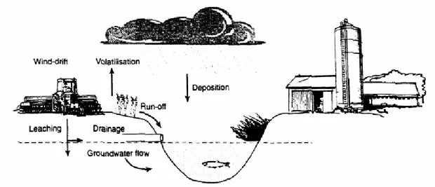
(18) 3.5.6 Pesticides Another important impact category in this type of study is pesticide use. The amount of used pesticides can be quantified, but the dangerousness of pesticides is more difficult to determine. Several methods have been developed to calculate the impact of pesticides on human health, aquatic and terrestrial ecosystems (Margini et al., 2002). In this study though, only a general view of how dangerous pesticides are will be given. In the impact assessment the amount of pesticides used in the scenarios will be accounted for. In order to determine the dangerousness of pesticides it is important to establish the mobility of the pesticides. In general, pesticides can be transported in the environment in five different ways: (see also Figure 4) 1. Wind-drift 2. Volatilisation 3. Deposition 4. Run-off 5. Transports in soil and water (for example via leaching and drainage). Figure 4. Principal environmental pathways by which agricultural pesticides may be transported to surface waters. After Kreuger (1999). Further, the pesticides can be spread in the environment due to negligence. The pesticides can be spilled, spread in unsuitable places or in incorrect ways or the equipment can be cleaned in a careless way. Even a few millilitres of a pesticide spilled on the farmyard can cause large effect on the environment. Imagine that 1 gram of active substance is spilled on a farmyard made of gravel. To dilute the pollution to 0.1 µg/l (the EU limit for presence of single pesticide in water), 10 000 m3 of water is needed (Fogelfors, 1995). There are today many reports of occurrence of pesticides in surface and ground waters. As long as pesticides have been used there have been traces in the environment of these substances. The most common effect of pesticides is in other words a general pollution of the 10.

(19) environment (Fogelfors, 1995). All substances that have an anthropogenic origin can be classified as environmental polluters. This does not necessarily mean that they are dangerous to human health or the environment. But the effect is very often not fully known. Pesticides can have an influence on the soil, soil organisms and biological soil processes. In most cases these effects are marginal compared to other cropping measures or “natural” factors. Many pesticides can have damaging effects on water organisms. Some substances are accumulated in the sediment and can cause problems during long time ahead (Fogelfors, 1995). For insects and game, the indirect effects of herbicide use are far more relevant that direct poisoning. The indirect effects can for example be the change of flora when herbicides are used (Fogelfors, 1995). Pesticides are used to fight living organisms and can be dangerous to humans. For the farmers, the pesticides can be taken in through skin and lungs or by accidental swallowing. The damage on the body can be of different kinds, irritation, acute poisoning, allergies etc (Fogelfors, 1995). For the general public, the health risks of pesticides are small according to the National Food Administration (Livsmedelsverket, www). The residues in agricultural products are only a few percent of the maximum intake limit. In drinking water there are more uncertainties. There is no judgement of how many people in Sweden that are exposed to pesticides in drinking water. But the majority of the population is not exposed to dangerous levels of pesticides in drinking water according to the National Food Administration.. 4 FARMING SYSTEMS Before the LCA is carried out, the farming systems need to be defined. The chemical farming system is based upon a farm in Tierp, Sweden. Most conditions are the same in the mechanical scenario, such as fertilisers and other chemicals besides herbicides. The difference between the scenarios is mainly the weed control. As the farm in Tierp do not use mechanical weed control, that part of the study is solely based upon literature studies. As mentioned earlier, in the LCA a mixture of what is appropriate in theory and what is actually done on the farm in Tierp will be used. 4.1 Crop sequence 4.1.1 Literature In Sweden’s climate, a good crop sequence is the base of a sustainable farming system. It is important for the outcome of the yield and affects the plant nutrition, soil humus content, fungus and insects. But it also affects the weeds (Fogelfors, 2001). In order to carry out a realistic LCA it is vital that a proper crop sequence is determined. The crop sequence has to be similar in both the scenarios. This means that it has to be a sequence that is suitable for both chemical and mechanical weed controls. As it seems, the mechanical scenario is the most dependent on a suitable crop sequence and so will be the determining system and the chemical scenario will just follow that order. So how does one determine a proper crop sequence for mechanical weed control? The first question that needs to be answered is how the crop sequence affects the weeds. According to several studies the chosen sequence is crucial for the amount and species of 11.

(20) weeds appearing on the field (Fogelfors, 1995 p18; Gummesson, 1992 and Hammar, 1990). To keep control of the weeds it is important that the sequence contains both winter and spring crops. The weeds that prefer winter crops and weeds that prefer spring crops are alternately favoured and disfavoured, making it hard for them to establish any larger populations. But most important of all is that the sequence contains cultivated grassland, ley. By alternating annual and perennial crops it is possible to control both the annual and perennial weeds (Fogelfors, 2001). What kind of weeds that appear are strongly related to the chosen crop. In literature relating to the subject following is said: Spring cereal crops: Barley is the most competitive spring crop because of its ability to grow side shoots and it’s well developed root system. Second best is oats and after that spring wheat (Fogelfors, 1995). Weeds that commonly appear in spring crops are Aventa fatua (wild oats), Chenopodium album (white pigweed), Polygonum aviculare (knotgrass), Stellaria media (chickweed), Elymus repens (couch grass), Equisetum arvense (common horsetail) and Cirsium arvense (field thistle) (Fogelfors, 2001). Winter cereal crops: Winter rye is labelled as the most competitive winter crop, due to its quick growth and its long straws. Rye seldom gives any problems with weeds. Second best is rye wheat followed by winter barley and winter wheat (Lundkvist & Fogelfors, 1999). Common weeds in winter crop are Polygonum aviculare (knotgrass), Matricaria Perforata Merat (scentless mayweed), Galium aparine (goose grass), Chamomilla recutita (camomile), Stellaria media (chickweed), Galeopsis (hemp nettle), Centaurea cyanus (cornflower), Myosotis arvensis (forget-me-not), Elymus repens (couch grass) and Apera spicaventi (silky bent grass). (Fogelfors, 2001) Potato: In the beginning of the growth season potato is a very weak weed competitor. It is then of great importance that mechanical tillage is conducted to fight annual weeds. But by the time the potatoes bloom the weeds are very difficult to maintain (Fogelfors, 1995). Ley: Cultivated grassland has in field experiments proven to be a very efficient weed controller. A crop sequence with ley has drastically fewer weeds than one without ley (Nilsson, 1992). The ley efficiently fights field thistle and corn thistle, under the condition that it is thick and in good growth (Gummesson, 1992). These two weeds are the most difficult to control without herbicides and are very resistant to mechanical tillage. Therefore it seems imperative to include ley in the crop sequence. Ley has also an inhibiting effect on the production of weed seeds and on the period of time the seeds are viable. (Gummesson, 1992). On the other hand, ley favours weeds such as Plantago major (broad-leafed plantain), Ranuculus repens (creeping buttercup), and Taraxacum vulgare (dandelion) (Fogelfors, 2001). Peas: Peas are not good competitors and can cause severe weed problems if appropriate weed control is not carried out. Weeds in peas very often cause harvest problems, particularly during rainy autumns. The peas lodge at an early state and can then be fully overgrown by weeds (Gummesson, 1992).. 12.

(21) 4.1.2 Chosen crop sequence Based on above knowledge the following crop sequence for both the chemical and the mechanical system is chosen as basis for the LCA-study: • • • • • •. Barley + under seed Ley Ι Ley II Winter Wheat Oats Potatoes. 4.2 Presentation of Fäcklinge Fors Farm Fäcklinge Fors farm is situated in Tierp in the province of Uppland in Sweden. Lars-Gunnar Sandin runs the farm. It includes 180 hectare of grown field and about 30 cows on extensive pasture. The soils are quite light, varying from loam to fine sand soil. The phosphorus storage is mainly in class III and IV, the potassium in class II and III. In the LCA the soil is presumed to be sandy loam in P-AL class III and K-AL class II. On the farm in Tierp barley, winter wheat, oats, potato and ley is grown in accordance with the earlier chosen crop sequence. The ley is harvested as both hay and silage, but in the LCA all ley is presumed to be harvested as silage. Some of the straw is harvested on Fäcklinge Fors farm, but in this study all straw is assumed to be incorporated in the soil. This means that no allocation has to be done between the crops and the straw. According to the farmer, the weeds that cause most problems on Fäcklinge Fors farm are Chenopodium (goosefoot), Elymus repens (couch grass), Lamium (dead nettle), Polygonum aviculare (knotgrass) and Galium aparine (goose grass). 4.3 Yields 4.3.1 Fäcklinge Fors The yield varies very much from year to year. As an average barley and oats gives rise to about 4 ton/ha, winter wheat 5-6 ton/ha, ley 5-6 ton/ha and potatoes approximately 25-30 ton/ha. 4.3.2 Literature The normal yield for conventional farming in the province of Uppland is presented in Table 1. Note that these yields will be used in the LCA and so represents the functional unit: the total harvest from all crops during one crop sequence.. 13.

(22) Table 1. Normal yields Uppland (Jordbruksverket, 2002). The yields are given as 15% water content for cereals and as dry weight for ley Crop Yield (kg/ha) Barley 4 436 Ley, total 6 586 1 Winter wheat 5 657 Oats 4 021 Potato 22 212 1. From Agriwise (www). First harvest 4 128 kg, second harvest 2 458 kg.. In the mechanical scenario the yields will probably be lower than in the chemical scenario. This is interesting because the functional unit is the total yield. So if the mechanical scenario gives rise to lower yields, a larger area of land will have to be cultivated to reach the same yield. This means more use of fossil fuels and other environmental effects. What yield that can be estimated in the mechanical scenario depends on a number of different factors. First of all, how and when the mechanical weed control is carried out. For example, harrowing usually has best effect on weeds in an early state, but if you harrow too early the crop might be damaged. The time of treatment is a very important factor. An evaluation between the effect on the weeds and the damage on the crops has to be done. Other things that affect the outcome of the yield with mechanical weed control are types of crop, type of weeds, variations in weather, seedbed preparations etc (Tersbøl et al., 1998). Since it is necessary to put figures on the losses to fulfil the life cycle assessment, it is important to estimate a reasonable loss. Between 1974 and 1988 a field trial was conducted in southern Sweden where mechanical and chemical weed control was compared to untreated field plots (Gummesson, 1990). The crop sequence consisted mainly of oats and barley, sometimes alternating with rye and wheat. The mechanical control consisted of harrowing. The results showed that the yields were lower in the mechanical plots than in the chemically treated as well as the untreated. The losses in mechanically treated fields were approximately 400 kg/ha in winter wheat, 420 kg/ha in barley and 450 kg/ha in oats as an average over the years. In other field experiments losses between 4-20 % has been noticed in oats and 7-40% losses in barley (Boström, 1999). These trials were also conducted with a very monotone crop sequence. In 2002 The Swedish Board of Agriculture published a report, a plan of action, for the usage of pesticides in Sweden (Emmerman et al., 2002). They estimated the losses in cereals to 250500 kg/ha as a consequence of larger number of weeds when pesticides are no longer used. For potatoes the losses were valued to 4 000 kg/ha. However, these estimations are based on a short time perspective and when no other weed control (direct or indirect) is applied. It is the loss that you can expect if you keep growing the same crops year after year and just stop using pesticides. These results show how difficult it is to switch to mechanical weed control in a crop sequence with only cereals. In this paper though, more effort is put on indirect weed control and the losses are not likely to be of the same magnitude. In Denmark a lot of research has been done on what losses to expect when herbicides are not used. In a report by Tersbøl et al. (1998) the estimated loss in spring crops is 0-15 % for mechanical weed control compared to chemical. In winter crops the same figure is 0-10 %. In. 14.

(23) potato cropping the same yield can be obtained with mechanical weed control as with chemical. In another Danish report (Mikkelsen et al., 1998) the losses when transferring from chemical to mechanical weed control are 11-16 % in winter wheat and 6-15 % in barley. The Danish government has decided to minimise the usage of chemicals in agriculture. A very comprehensive investigation, the Bichel-study, was conducted. In this report (Bicheludvalget, www) approximations of losses as a consequence of switching to mechanical weed control are declared. In winter wheat the losses are estimated to 13%, in barley 8 %, in potatoes 0 % and in oats 9 %. These figures are based on a few Danish trials, but mostly upon expertise judgement. For ley the decrease in yield are probably not of any larger significance. Emmerman et al. (2002) calculates that the yield is lowered by 3% if all chemical treatment is ceased. In field trials it has been proven that there is no difference in yields from ley in farming systems with chemical and mechanical weed control (Fischer and Hallgren, 1991). In this study it is estimated that the yields in the mechanical system is lowered by 10 % in barley, 0% in ley, 12% in winter wheat, 10% in oats and 0% in potatoes. 4.3.3 Chosen yields The chosen yields in the chemical and mechanical scenarios as well as the used area of land are presented in Table 2. Note that the yields in the table also represent the functional unit. Table 2. Yields and used land Chemical scenario Yield Land (kg/ha) use (ha) Barley 4 436 1. Mechanical scenario Yield total Yield Land Yield total (kg) (kg/ha) use (kg) (ha) 4 436 3 992 1.11 4 436. Ley I Ley II Winter wheat Oats Potato Sum (functional unit). 6 586 6 586 5 657 4 021 22 212 49 498. 6 586 6 586 5 657 4 021 22 212. 1 1 1 1 1 6. 6 586 6 586 4 978 3 619 22 212. 1 1 1.14 1.11 1 6.36. 6 586 6 586 5 657 4 021 22 212 49 498. 4.4 Fertilisers The needed rate of fertilisers is strongly related to the yield. The yields in the mechanical scenario are lower per hectare and subsequently the needed amount of fertilisers per hectare. 4.4.1 Fäcklinge Fors The fields on Fäcklinge Fors farm do not have any larger storage of potassium or phosphorus and continuously needs to be fertilised. On most cereal fields, the commercial fertiliser NPK 24-4-5 is used. In winter wheat additional nitrogen is also added; Axan (NS 27-3). 15.

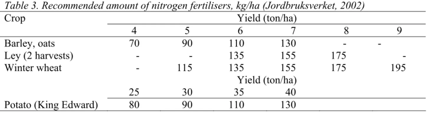
(24) In potato (King Edward) the commercial fertiliser NPK 8-5-19 is applied. In ley, fertilisers are spread in two rounds. The first time NPK 24-4-5 is applied and the second time Axan is spread. 4.4.2 Literature Jordbruksverket, the Swedish board of agriculture gives the following recommendations for nitrogen fertilisation: Table 3. Recommended amount of nitrogen fertilisers, kg/ha (Jordbruksverket, 2002) Crop Yield (ton/ha) 4 5 6 7 8 Barley, oats 70 90 110 130 Ley (2 harvests) 135 155 175 Winter wheat 115 135 155 175 Yield (ton/ha) 25 30 35 40 Potato (King Edward) 80 90 110 130. 9 195. For phosphorus and potassium the recommendations are based upon in which P-AL and KAL classes the soil is placed. Jordbruksverket (2002) gives the following recommendations for P-AL class III and K-AL class II: Table 4. Recommended amount of phosphorus and potassium Crop Yields P (ton/ha) (kg/ha) Cereals 5 15 Ley I 6 15 Ley II 6 15 Potato 30 601. K (kg/ha) 45 2 90 140 160. 1. Sufficient for the two following crops 2. If straw is removed the dose is raised by 20 kg K/ha. The amount of P- and K-fertilisers are adjusted to the yield by adding or subtracting 3 kg phosphorus and 5 kg potassium per ton divergent cereal, 0.5 kg phosphorus and 4 kg potassium per ton potato and 20 kg potassium per ton divergent ley. 4.2.3 Chosen fertilisers In Table 5 the chosen amount of fertilisers per hectare is shown. These are the data that will be used in the calculations of the LCA. The fertilisers are chosen solely on basis of the recommendations in the literature review.. 16.

(25) Table 5. Chosen fertiliser strategy per hectare. Since the yields are lower in the mechanical scenario, the amounts of fertilisers are lower per hectare Chemical scenario Mechanical scenario N P K N P K (kg/ha) (kg/ha) (kg/ha) (kg/ha) (kg/ha) (kg/ha) Barley 79 13 42 70 12 40 Ley I 145 17 93 145 17 93 Ley II 145 17 143 145 17 143 Winter wheat 128 17 48 115 15 45 Oats 70 12 40 62 11 38 Potato 80 56 130 80 56 130 4.5 Seed 4.5.1 Fäcklinge Fors The following varieties are used: Table 6. Varieties on Fäcklinge Fors Farm Crop Variety Barley Cecilia and Baronesse Ley SW 944 Winter wheat Kosack Oats Sang Potato King Edward and Bintje 4.5.2 Literature The suitable amounts of seed are according to Odal listed in Table 7 (Andersson, 2001). Odal is a Swedish farmer owned cooperation which mainly deals with cereals. Table 7. Amount of seed Crop Barley (two-row) Ley Winter wheat Oats Potato. Seed (kg/ha) 180 20-25 210 205 2 200-3 700. 4.5.3 Chosen amount of seed The procedure for sowing is the same in the chemical and the mechanical scenario for all crops except ley. In the chemical scenario the ley seeds are sown just after the barley. In the mechanical scenario though, the sowing of ley is postponed. The sowing is instead done in connection with a weed harrowing before the emergence of the crop. The chosen amount of seed is in accordance with Table 7; ley is assumed 20 kg and potato 2 750 kg.. 17.

(26) 4.6 Tillage operations The aim of tillage operations is to prepare the soil for a certain crop. The tillage operations are the same in both the chemical and the mechanical scenario. Some of these operations also have an effect on weeds and could just as well have been included in the weed control chapters. But since the operations are the same in both the scenarios there is a point in treating them together.. 4.6.1 Literature Ploughing. In the autumn there is a need to loosen the soil after the compacting during summer. Crop residues are buried; down under the soil the organic substances are faster metabolised. Ploughing is also effective in fighting perennial weeds. The plough cuts off the roots and under-ground stems of the weeds and turns the soil over. Seedbed preparation. Before sowing the soil has to be prepared. The wanted result from seedbed preparation is •. a smooth soil surface. •. small soil particles. •. sorted soil; the finest particles closest to the seedbed bottom. •. the right sow depth. •. a smooth seedbed bottom. •. weed control. This can be done with different types of harrows, levelling boards, cage rollers and disc tools. Ridging. Ridging is mainly done in potato cropping to cover the potatoes and protect them from sunlight. Also, annual and perennial weeds are fought. An amount of soil is moved to cover the potatoes and at the same time weeds are pulled up or covered by soil. Stubble cultivation. Stubble cultivation is done in both the chemical and mechanical scenario when the ley is terminated. It is necessary to stubble cultivate in order to cut the plant residues and mix them properly with the soil before the winter wheat is sowed. 4.7 Pesticides 4.7.1 Fäcklinge Fors The following pesticides are used on the farm: Tilt Top 500 EC (fungicide), Stereo 312.5 EC (fungicide), Sumi-Alpha 5 FW (insecticide), Epok 600 EC (against downy mildew), Shirlan (against downy mildew) and Reglone (haulm killer). The dose is regulated by need, an evaluation done by the farmer on site. 4.7.2 Literature As the types of pesticides used on Fäcklinge Fors farm can be considered as quite representative for a conventional Swedish farm, these data will be used (Andersson, 2001). The rate of the pesticides will on the other hand be determined from literature, Agriwise (www) and Anderson, 2001. The normal rates of the above pesticides are presented in Table 8. 18.

(27) 4.7.3 Chosen pesticides The time perspective in this LCA is one year. But some consideration has to be made for the longer time perspective. For instant, some pesticides are not used on every field every year; reducing the number of occasions to less than one represents this. For example, if the number of occasions is 0.3 the pesticide is used every third year.. Table 8. Crop, pesticide and dose per hectare Crop Product Number of occasions x dose (l) Barley Sumi-Alpha 5 FW 0.3 x 0.3 Stereo 312.5 EC 0.3 x 1.0 Ley. -. Active substance Active substance (g/ha) Esfenvalerat 45 Cyprodynil + 94 propikonazol. -. Winter wheat Sumi-Alpha 5 FW Tilt Top 500 EC. 0.3 x 0.3 1 x 0.8. Esfenvalerat Propikonazol + fenpropimorf. 45 400. Oats. Sumi-Alpha 5 FW Tilt Top 500 EC. 0.3 x 0.3 0.2 x 0.8. Esfenvalerat Propikonazol + fenpropimorf. 45 80. Potato. Sumi-Alpha 5 FW Shirlan Reglone Epok 600 EC. 0.3 x 0.3 5 x 0.35 2x3 2 x 0.45. Esfenvalerat Fluazinam Dikvat Mefenoxam + fluazinam. 45 875 1200 540. 4.8 Chemical weed control 4.8.1 Fäcklinge Fors On Fäcklinge the following chemicals are used for weed control: Harmony Plus 50 T, Express 50 T, Ariane S, Starane 180. Hormotex 750. Sencor, Titus 25 DF and Roundup. 4.8.2 Literature As the types of herbicides used on Fäcklinge Fors farm are quite representative, these data will be used. But the rate of the herbicides will be determined by studying literature. The normal rates for the above herbicides are presented in Table 9 (Agriwise, www; Anderson, 2001).. 19.

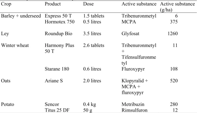
(28) 4.8.3 Chosen chemical weed control In Table 9 the chosen herbicides and doses are presented. Table 9. Crop, herbicide and dose per hectare Crop Product Dose Barley + underseed Express 50 T Hormotex 750. 1.5 tablets 0.5 litres. Active substance Active substance (g/ha) Tribenuronmetyl 6 MCPA 375. Ley. Roundup Bio. 3.5 litres. Glyfosat. Winter wheat. Harmony Plus 50 T. 2.6 tablets. Starane 180. 0.6 litres. Tribenuronmetyl + Tifensulfuronme tyl Fluroxypyr. Oats. Ariane S. 2.0 litres. Klopyralid + MCPA + fluroxypyr. 520. Potato. Sencor Titus 25 DF. 0.4 kg 50 g. Metribuzin Rimsulfuron. 280 12. 1260 11. 108. 4.9 Mechanical weed control 4.9.1 Literature The most important tool to fight weeds is the indirect measures taken in the farming system. But it is also important to fight the weeds directly in order to ensure that the existing weeds do not multiply. The following direct mechanical weed control is common: Stubble cultivation. By stubble cultivating with disc tools, cultivator or alike as soon as possible after harvest perennials can be fought, mainly couch grass and other vegetative propagated weeds. The effect on annual weeds is limited. The best effect is reached if the tillage is repeated after a few weeks and followed by ploughing (Fogelfors, 1995). Weed harrowing. There are mainly three types of weed harrowing (Lundkvist and Fogelfors, 1999): •. Blind harrowing. Blind harrowing means that you harrow after sowing but before the emergence of the crop.. •. Harrowing after the emergence of the crop. This should not be done when the crop has just emerged (1-2- leaf-stage) but rather in 3-leaf-stage.. •. Selective harrowing. Selective harrowing is conducted with a long-tine harrow in crops that grow in dense rows, for example when the cereal starts its stem elongation.. Harrowing fights weeds by tilling the top layer of soil. Weeds are most sensitive to harrowing in their early stages as soil covers them. Generally annual weeds like Chamomilla recutita 20.

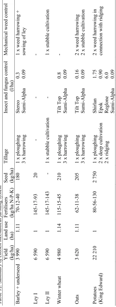
(29) (camomile), Papaver (poppy) and Vioala arvensis (field pansy) are sensitive to harrowing, while it has little effect on perennials. Weeds usually germinate and establish under longer periods than the crops. It is therefore sometimes advisable to harrow several times to reach good effects against weeds (Fogelfors, 1995). How many times the harrowing should be conducted depend on type of soil and the current weed-pressure. Tersbøl et al. (1998) recommends in spring cereal crops with high weed-pressure, one blind harrowing and 1-2 harrowings after the emergence of the crop. In winter crops they recommend one blind harrowing and 2-3 selective harrowing. The timing of the weed harrowing is crucial for the result. The difference in size between the crop and the weed has to be optimal. The harrowing should take place when the weed is as small as possible, but the crop has to be large enough not to take to much damage. When this time occurs depends on amount and composition of weeds, type of crop, soil and climate (Mattsson and Sandström, 1994). In spring crops it is possible to wait with the sowing of under-seed ley. This gives the opportunity to weed harrow one time in connection to the sowing of the ley-seed. In potatoes the weed harrowing and the ridging is done together in one instant. Inter-row hoeing. Inter-row hoeing chops off the weeds and at the same time loosen the soil. The weeds are fought by cutting off the roots, being covered by soil or by being pulled up. Inter-row hoeing is gentler to the crop than harrowing. Inter-row hoeing can be done in crops that are planted with large distances between the rows, such as sugar beets, potatoes and vegetables. It can also be done in cereals, but only if the distance between the rows are large enough, at least 17-20 cm, which is rather unusual. Inter-row hoeing is best done while the weeds are small, but the timing is not so important as in harrowing (Lundkvist and Fogelfors, 1999). Mowing. Weeds can also be cut of with a mower. This is common in organic farming systems where field thistle is a problem weed. By cutting of the thistle it is restrained from propagating (Bovin, www). 4.9.2 Chosen mechanical weed control As mentioned earlier, weed control in a farming system consists of both direct and indirect actions. In Table 10 the direct weed control that differs from the chemical scenario is listed. This weed control strategy is put forward in co-operation with Maria Wivstad (pers. com). Table 10. Mechanical weed control for a crop sequence Crop Mechanical weed control Barley 1 x weed harrowing Ley I Ley II 1 x stubble cultivation Winter wheat Oats 2 x weed harrowing 2 x stubble cultivation Potato 2 x weed harrowing. 4.10 Summary of chosen farming systems A summary of the determined farming systems is presented in Table 11 and 12. 21.

(30) 4 440. 6 590. 6 590. 5 660. 4 020. 22 210. Barley + underseed. Ley I. Ley II. Winter wheat. Oats. Potatoes (King Edward). 80-56-130. 70-12-40. 128-17-48. 145-17-143. 145-17-93. 79-13-42. 2 750. 205. 210. -. 20. 180. Table 11. Summary of chosen conventional farming system Yield Fertilisers Seed (kg/ha) (kg/ha N-P-K) (kg/ha). 22. 1.75 0.90 6.0 0.09. Tilt Top 0.16 Sumi-Alpha 0.09. Tilt Top 0.8 Sumi-Alpha 0.09. -. -. Insect and fungus control (l/ha) Stereo 0.3 Sumi-Alpha 0.09. 1 x ploughing Shirlan 2 x deep cultivation Epok 2 x ridging Reglone Sumi-Alpha. 1 x ploughing 3 x harrowing. 1 x ploughing 3 x harrowing. 1 x stubble cultivation. -. 1 x ploughing 3 x harrowing. Tillage. 3.5. Sencor Titus. Ariane S. 0.4 50 g. 2.0. Ariane S 3.0 Hormotex 750 2.0. Roundup Bio. -. Harmony Plus 1.5 tablet Starane 180 0.4. Chemical weed control (l/ha).

(31) 6 590. 6 590. 4 980. 3 620. 22 210. Ley I. Ley II. Winter wheat. Oats. Potatoes (King Edward). 1. 1.11. 1.14. 1. 1. 80-56-130. 62-11-38. 115-15-45. 145-17-143. 145-17-93. 2 750. 205. 210. -. 20. 23. 1 x ploughing 2 x deep cultivation 2 x ridging. 1 x ploughing 3 x harrowing. 1 x ploughing 3 x harrowing. 1 x stubble cultivation. -. Table 12. Summary of chosen mechanical farming system Yield Land use Fertilisers Seed Tillage (kg/ha) (ha) (kg/ha N-P-K) (kg/ha) Barley + underseed 3 990 1.11 70-12-40 180 1 x ploughing 3 x harrowing. Shirlan Epok Reglone Sumi-Alpha. Tilt Top Sumi-Alpha. Tilt Top Sumi-Alpha. -. -. 1.75 0.90 6.0 0.09. 0.16 0.09. 0.8 0.09. Insect and fungus control (l/ha) Stereo 0.3 Sumi-Alpha 0.09. 2 x weed harrowing in connection with ridging. 2 x weed harrowing 2 x stubble cultivation. -. 1 x stubble cultivation. -. 1 x weed harrowing + sowing of ley. Mechanical weed control.

(32) 5 INVENTORY OF FARMING SYSTEMS In this chapter data will be gathered and presented. A concluding datasheet for the emissions of each crop is presented in Appendix 7-17. 5.1 Field operations Data for fuel consumption and emissions when performing field operations are taken from JTI, the Swedish Institute for Agricultural and Environmental Engineering, a report by Lindgren et al. (2002), see Appendix 2. The data is collected from a Valtra 6600 tractor on heavy clay. The soils at the studied farm is of a lighter kind and operations like ploughing should give rise to a little lower fuel consumption, but since such data is not available these are the figures that will be used. The JTI-report does not cover emissions of SOx. These emissions are instead based on content of sulphur in the fuel. According to Hansson and Mattsson (1999) the emissions can be estimated to 0.0935g SO2/MJ. There are no measurements of fuel consumption for spraying in the report from JTI. According to Hansson and Mattsson (1999) the load at spraying can be assumed to be equivalent to the load at sowing. The ley is harvested as silage with a mower conditioner. The grass is pressed to round bales and then coated with stretch film. There are no figures on how many hectares per hour a stretch film device can do in the JTI-report but the emissions per hour is given (Lindgren et al., 2002). According to Magnus Lindgren (pers. com.) the average speed can be estimated to 5 km/h for such operations and the working width the same as for the mower conditioner. For potato cropping, figures from Mattsson et al. (2002) has been used for fuel consumption in field operations (Appendix 2). The emissions on the other hand were calculated from Lindgren et al. (2002) for operations that are similar, for example were potato-planting set equal as stubble cultivation. Transports to and from fields to farm are calculated by adding 10% of field operations. 5.2 Diesel production The production and distribution of diesel are accounted for in this LCA. Figures are taken from Uppenberg et.al. (2001) and are presented in Appendix 3. 5.3 Electricity production Data for production of electricity are taken from Uppenberg et al. (2001) and are presented in Appendix 3. The data is based on average Swedish electricity during 1999. produced by 48.2 % hydropower and 44.3 % nuclear power. 5.5 Pesticide and herbicide production There are very scarce data on energy use and emissions from pesticide production. In this study, figures from Kaltschmitt & Reinhardt (1997) were used. The data are given as emissions per kilogram active substance, not regarding type of substance (Appendix 4).. 24.

(33) 5.4 Mineral fertiliser production Producing mineral fertilisers requires energy. Especially the production of nitrogen fertilisers requires large amounts of energy, mostly carried by natural gas. A number of substances are also emitted to air and water in the processes of making mineral fertilisers. Davis & Haglund (1999) have investigated this, see Appendix 5. The fertilisers are assumed to be manufactured in Köping, Sweden. The distance between Köping and Tierp is 175 kilometres and the fertilisers are transported by truck. The emissions from the transports are based on data from NTM, the Network for Transport and the Environment (www), presented in Appendix 5. 5.6 Seed production For cereals as well as potatoes, the production of seed does not differ substantially from ordinary cultivation. In this study, the figures from cereal production that already has been calculated will be used. Seeds in barley, winter wheat, oats and potato will be net calculated and increased by 10% to compensate for higher cultivation costs in seed production. For cereal seed production 10 % is commonly used (Cederberg, 1998). The production of ley seed differs significantly from cultivation of ley for silage. The production of grass and clover was thoroughly investigated by Cederberg (1998) and calculations in this study are based on those data. 5.7 Production of stretch film The harvested ley is pressed to round bales and then covered with plastic stretch film. The use of stretch film is estimated to 4.3 g per kg dry substance of ley by JTI (Dalemo et al., 1997). The stretch film is assumed to be produced of LDPE (low density polyethylene). Data for production and handling of waste (to landfill) for LDPE are taken from Tillman el al. (1991) and are presented in Appendix 6. 5.8 Emissions of N in cropping In agricultural production, emissions of ammonia (NH3), nitrous oxide (N2O) and nitrate (NO3-) can have large influence on acidification, eutrophication and the atmosphere’s radiate balance. It is therefore of great importance that these emissions are correctly calculated. Unfortunately, accurate data is hard to obtain since the sizes of the emissions are strongly influenced by climate, type of soil and fertilisers and how the fertilisers (manure) are handled (Cederberg, 1998). 5.8.1 Nitrate (NO3-N) Dissolved nitrogen easily follows the water movement trough the soil. Leaching of NO3occurs when surplus water is drained away, mainly during winter season. The climate has a large influence on the N-leaching. The amount of precipitation and the temperature during autumn determines the amount lost N. The type of soil can also have influence on the Nleaching; lighter soils are more inclined to leach than clay soils (STANK). Further, there is a connection between tillage and N-losses. When the soil is cultivated large soil aggregates are crushed to smaller pieces. This means that the microorganisms in the soil get a larger active surface to work on. Also, air and warmth is baked in to the soil. Theses two factors together lead to a larger mineralization and a larger risk of leaching ( STANK).. 25.

(34) The N-leaching is in this study calculated in accordance with the STANK-model by the formula: N-leaching = basic leaching x crop factor x cultivation factor + manure effect + effect of fertilising intensity The basic leaching is determined by geographic location, precipitation and soil type. The crop factor is determined by type of crop. Crops like potato and peas have a high factor since they are more inclined to leach due to the sparse growing. The cultivation factor is set to adjust for the difference between early and late autumn tillage. An early tillage gives a higher factor. The effect of spreading manure is determined by geographic location, type of soil and crop. The effect of fertilising intensity accounts for the increase in N-leaching when the amount of applied fertilisers is larger than the recommended amounts. 5.8.2 Ammonia (NH3) Losses of ammonia in agricultural production mainly occur while spreading manure. NH3 emissions from mineral fertilisers are generally small, depending on the pH of the soil. Tidåker (2003) points out that the figure varies between 0.2% and 1% in different studies. In this study the average figure 0.6% of applied mineral fertilisers is used. 5.8.3 Nitrous oxide (N2O) Emissions of nitrous oxide occur from natural processes in the conversion of nitrogen. Nitrous oxide is also emitted from agricultural land when fertilisers are added to the soil. As N2O has a very high global warming potential (296 CO2-equivalents) it will have an impact on the result of global warming. The loss of N2O from the soil is calculated in accordance with the IPPC guidelines; 1.25% of total added nitrogen is emitted as N2O-N (IPPC, 1997). Further, there are also indirect emissions of N2O. Emissions of nitrate and ammonia go through the nitrogen cycle and hereby production of N2O will occur. According to IPPC (1997) these indirect emissions can be calculated by adding 0.01 kg N2O per kg NH3 and 0.025 kg N2O per kg NO3-. In Table 13 a summary of the N emissions is presented.. Table 13. Emissions of N from field for chemical scenario. Numbers in parenthesis are for the mechanical scenario when differing between the scenarios Applied amount of NO3NH3 N2O N2O indirect nitrogen fertiliser (g/ha) (g/ha) (g/ha) (g/ha) (kg/ha) Barley 80 (72) 10 500 480 (432) 1 000 (900) 267 Ley I 145 8 750 870 1 813 227 Ley II 105 26 250 630 1 313 663 Winter wheat 130 (114) 17 500 780 (686) 1 625 (1 425) 445 Oats 70 (63) 17 500 420 (378) 875 (788) 442 Potato 80 29 750 480 1 000 749. 26.

No results found