LiU Working Papers in Economics
No. 7 | 2020
Asymmetric Dynamics between
Uncertainty and Unemployment Flows in
the United States
Ali Ahmed
Mark Granberg
Victor Troster
Gazi Salah Uddin
LiU Working Papers in Economics are circulated for discussion and comments only. They have not undergone the typical referee process for publication in a scientific journal and they may not be reproduced without permission of the authors.
Division of Economics
Department of Management and Engineering Linköping University
Asymmetric Dynamics between Uncertainty and Unemployment Flows in the United States
Abstract
This paper examines how different uncertainty measures affect the unemployment level, inflow, and outflow in the U.S. across all states of the business cycle. We employ linear and nonlinear causality-in-quantile tests to capture a complete picture of the effect of uncertainty on U.S. unemployment. To verify whether there are any common effects across different uncertainty measures, we use monthly data on four uncertainty measures and on U.S. unemployment from January 1997 to August 2018. Our results corroborate the general predictions from a search and matching framework of how uncertainty affects unemployment and its flows. Fluctuations in uncertainty generate increases (upper-quantile changes) in the unemployment level and in the inflow. Conversely, shocks to uncertainty have a negative impact on U.S. unemployment outflow. Therefore, the effect of uncertainty is asymmetric depending on the states (quantiles) of U.S. unemployment and on the adopted unemployment measure. Our findings suggest state-contingent policies to stabilize the unemployment level when large uncertainty shocks occur.
Keywords: Uncertainty; Unemployment; Nonlinear dynamics; Granger-causality; Quantile
regression; U.S. labor market.
1. Introduction
Theoretical and empirical work has shown that uncertainty affects many aspects of the economy. For example, uncertain times make firms postpone their investments to more certain times (Bernanke, 1983; Dixit and Pindyk, 1994; Calcagnini and Saltari, 2000; Bloom et al., 2007; Antonakakis et al., 2015). Uncertainty also makes households reduce their consumption (Zhang and Wan, 2004), and it has an adverse effect on economic activity (Pastor and Veronesi, 2012; Bachmann et al., 2013; Pastor and Veronesi, 2013; Fernández-Villaverde et al., 2015; Leduc and Liu, 2016; Basu and Bundick, 2017; Choi, 2017). Moreover, uncertainty affects the unemployment level (Bloom, 2009; Abaidoo, 2012; Bachmann and Bayer, 2013; Ghosal and Ye, 2015; Jurado et al., 2015; Baker et al., 2016; Bloom et al., 2018; Mumtaz, 2018), and the effect of uncertainty on the unemployment level seems to be nonlinear over the business cycle (Morley and Piger, 2012; Caggiano et al., 2014; Nodari, 2014; Jones and Enders, 2016; Scotti, 2016; Caggiano et al., 2017a; Chatterjee, 2019). Nevertheless, empirical work on the relationship between the flows of unemployment and uncertainty is lacking,1 even though researchers have pointed out the importance of labor market flows when analyzing unemployment in general (Mortensen and Pissarides, 1994; Shimer, 2012; Elsby et al., 2013; Schaal, 2017). The unemployment rate is the ratio of the labor force without a job, which is a nonlinear result of two flows: the rate of job separation (inflow) and the rate of job finding (outflow). To the best of our knowledge, this is the first paper that analyzes how financial and economic uncertainties relate to these flows of unemployment and whether the observed nonlinear relationship between uncertainty and unemployment level can be explained by a linear relation between uncertainty and unemployment flows.
This paper examines how different uncertainty measures affect flows in and out of U.S. unemployment, whether those relationships are nonlinear, and if there are any common effects across uncertainty measures. Considering unemployment flows is important because few policy measures can be targeted directly at the unemployment level. Conversely, policy measures that affect hiring or firing rates are feasible. Moreover, previous studies on uncertainty and unemployment have used various measures of uncertainty, but little is known about how
1 Schaal (2017) does construct and test a search and matching model in which the effect of uncertainty on
unemployment flows are considered. To our knowledge, other articles that deal with the uncertainty-unemployment relationship (e.g., Bloom, 2009; Abaidoo, 2012; Bachmann and Bayer, 2013; Jurado et al., 2015; Baker et al., 2016; Bloom et al., 2018; Mumtaz, 2018) all focus on the unemployment level instead of flows.
different types of uncertainty affect unemployment comparatively. To address this issue, we need a comparative assessment of how various types of uncertainty relate to unemployment and its flows.
Furthermore, previous research papers on the impacts of uncertainty on U.S. unemployment have focused on effects at the mean or on impulse responses (e.g. Bloom, 2009; Schaal, 2017). To achieve a broader picture, we need to evaluate how the effects of uncertainty differ across the entire conditional distribution of unemployment and its flows. Tail-causality may be different than mean-causality. For instance, Lee & Yang (2012) found strong Granger-causality running from money to income in the U.S. in the tails of the distribution; yet there was only weak causality at the mean. Besides, we fully analyze Granger-causality between uncertainty and unemployment as the quantiles fully determine Granger-causality in distribution. Finally, the quantile-causality analysis verifies whether effects of uncertainty on unemployment are symmetric over different states (quantiles) of the U.S. economy. To our knowledge, only the work of Gupta et al. (2018) analyzes how uncertainty shocks affect the U.S. economic activity using a quantile regression framework. However, they overlook Granger-causality-in-quantile tests between uncertainty and unemployment and nonlinear specifications. Our results are relevant for scholars and policymakers alike to develop useful macroeconomic models and make accurate forecasts, and detailing the asymmetric dynamics on the uncertainty-unemployment relationship will help both of these endeavors.
In sum, we address three questions concerning the relationship between uncertainty and unemployment that have not been tackled in earlier work: (i) how does uncertainty relate to unemployment inflows and outflows? (ii) Which type of uncertainty affects the inflows and outflows of unemployment? And, (iii) are the impacts of uncertainty to unemployment significantly nonlinear along the business cycle? We contribute to the previous literature by examining the relationship between various uncertainty measures and unemployment inflows and outflows, and by utilizing a methodological approach proposed by Troster (2018), which analyzes Granger-causality between two variables over the entire conditional distribution. We use monthly data on unemployment level, inflow, and outflow in the U.S. over a period of 21 years. For the same period, we use four different uncertainty measures to capture financial, political, and geopolitical uncertainties (Volatility Index, Financial Stress Index, U.S. Economic Policy Uncertainty Index, and Global Economic Policy Uncertainty Index).
In line with macroeconomic theory, we find that fluctuations in uncertainty lead to increases in the unemployment level, increases in inflow, and decreases in outflow. These effects are stronger for inflow than for outflow, indicating that the inflow is the main driver in the connection between uncertainty and the unemployment level. U.S. uncertainty measures exhibit a stronger connection to all three unemployment indicators compared with the global uncertainty indicator. Our findings corroborate previous results of nonlinear impacts of uncertainty on the unemployment level (Caggiano et al., 2014; Nodari, 2014; Caggiano et al., 2017a, 2017b). However, the relation between uncertainty and unemployment flows is linear. We also find that uncertainty enhances the out-of-sample predictability of unemployment at extreme states (quantiles) of the U.S. economy.
The rest of this paper is organized as follows. Section 2 describes the theoretical framework of the effects of uncertainty on unemployment. Section 3 explains the econometric methodology with a particular focus on the quantile Granger-causality testing approach. Section 4 presents the results and discussion. Finally, Section 5 concludes the paper.
2. Theoretical Framework of the Uncertainty-Unemployment Relationship
In modern labor market theory, unemployment is analyzed in a search and matching framework with frictions (Pissarides, 2000); this framework has been also used to examine unemployment flow dynamics and firm characteristics (Davis et al., 2013), the effects of trade policy (Cosar et al., 2016), or life cycle wage growth (Lagakos et al., 2018), to name a few recent applications. These search and matching models focus on a matching function and acknowledge that it takes both time and money for a worker and a firm to find a mutually beneficial match. A significant characteristic of these search and matching models is that transitions between different states in the labor market are made explicit, e.g., the rates of job separation and job finding. For a more extensive survey of the search and matching literature and its role in macroeconomics, see Yashiv (2007). For our purposes, stating the relationship between the ins and outs of unemployment suffices to show why disaggregating the unemployment level is valid.
Accounting for entry and exit from the labor force is outside the scope of this paper. Following Yashiv (2007), let 𝑢 be the ratio of unemployed workers in the economy, 𝜆 the rate of job
separation, and 𝑝 the probability of finding a job. Then, the change in unemployment between two arbitrary periods, 𝑢̇, can be expressed as
𝑢̇ = 𝜆(1 − 𝑢) − 𝑝𝑢. (1)
The unemployment rate between periods does not change when the economy is in a steady state, which means that 𝑢 can be represented by the following equation in equilibrium:
𝑢 = 𝜆
𝜆 + 𝑝. (2)
Equation (2) shows how closely related job separation, job finding, and the level of unemployment are. It also demonstrates how unemployment may be disaggregated into its two flows. Further, as 𝜆 and 𝑝 are the in- and outflows to unemployment (𝑢), Equation (2) illustrates that the flows are nonlinearly related to unemployment in equilibrium.
Next, what role does uncertainty play in these unemployment flows? If we assume some wage rigidity and a standard Mortensen and Pissarides (1994) search and matching framework with frictions, the immediate response to uncertainty is that firms adjust their current labor stock. If capital and wages are rigid, firms are unable to adjust them quickly in response to a change in uncertainty. Firms can either hire or fire workforce.
Bloom (2014) argues that uncertainty influences the economy in general and unemployment in particular through three main channels: real option, risk premium, and risk aversion. As regards real option, suppose that the hiring decisions firms make are irreversible investments and that information necessary to pursue long-run projects comes over time so that waiting may improve hiring decision outcomes (i.e., there is uncertainty). Under these conditions, one can show that cyclical investment fluctuations will arise (Bernanke, 1983). This implies that firms would hire less people in periods of increased uncertainty because the returns on hiring workers would be uncertain and there would be an outside option, which is to wait for more information. Hence, the option value of delaying hiring decisions is high during periods of high uncertainty. If firms choose to wait for more information, the result is a reduced outflow out of unemployment in uncertain times. Firms may also be uncertain about the value of their current contracts during a
shock, which would increase the rate of separation for workers (for more details, see Chen and Funke, 2004).
As regards risk premium and risk aversion, the perceived risk of investments is high when uncertainty is high, increasing risk premia, which will lower overall investments if people are risk averse. For instance, Panousi and Papanikolaou (2012) show that investments tend to drop in uncertain times, especially in firms where managers own a larger share of the firm. This implies that managers tend to be risk averse, especially when risks are not properly diversified, which is more common as CEO compensation packages have increasingly come to include incentives such as stocks and options in the firm (Hall and Liebman, 1998; Gayle et al., 2015). As these CEOs can be instrumental in large hiring and firing decisions, lower diversification in combination with fluctuations in uncertainty may have direct effects on a firm’s hiring and firing rates.
All three channels generate the same predictions: If the labor decisions of firms are considered analogous to investment decisions, then increased uncertainty will lead to an increased unemployment level, an increased unemployment inflow, and a decreased unemployment outflow. These linear effects of uncertainty on 𝜆 and 𝑝 in Equation (2) imply that the theoretical impact of uncertainty on 𝑢 is nonlinear. These theoretical arguments explain the potential causal linkages between uncertainty and the unemployment flows. Such theoretical arguments would be difficult to construct between uncertainty and the unemployment level, without going through the inflow and the outflow to unemployment as they mostly affect the observed unemployment level. Therefore, considering unemployment flows is crucial to investigate the uncertainty-unemployment relationship.
3. Linear and Nonlinear Granger-Causality Tests
Let UNC0 = Z0 represent any of our four uncertainty measures, and UNE0 = Y0 represent any of our three unemployment measures. Let ℱ056≡ (ℱ0568 , ℱ056: ); ∈ ℝ> be the past information sets
of Y0 and Z0, with ℱ0568 ≡ (Y
056, … , Y05>) and ℱ056: ≡ (Z056, … , Z05>). We define the
conditional distribution of Y0 given ℱ056 as F8A(y|ℱ0568 , ℱ
056: ). The null hypothesis of
Granger-non-causality from Z0(uncertainty) to Y0 (unemployment), denoted as Z ↛ Y, can be defined as follows (Granger, 1969, 1980):
𝐻FG↛H ∶ 𝐹
8A(𝑦|ℱL56H , ℱL56G ) = 𝐹HM(𝑦|ℱL56H ), ∀y ∈ ℝ. (3)
Equation (3) defines Granger-non-causality in distribution, but certain studies only test for Granger-non-causality in mean, i.e.
𝐸(𝑌L|ℱL56H , ℱ
L56G ) = 𝐸(𝑌L|ℱL56H ), almost surely, (4)
where 𝐸(𝑌L|ℱ056H , ℱ
056G ) and 𝐸(𝑌L|ℱ056H ) are the conditional means of 𝑌L given ℱ056 and ℱ056H ,
respectively. Then, we first employ a linear F-test (of Granger-non-causality in mean) on the estimated coefficients of bivariate vector autoregressive (VAR) models, to test whether HF: βT = 0, for all j = 1,…, q, as follows:
𝑌L= U 𝛼W𝑌L5W X W + U 𝛽W𝑍L5W X W + 𝜀L, (5) 𝑍L = U 𝛼W∗𝑌 L5W X W + U 𝛽W∗𝑍 L5W X W + 𝜀L∗, (6)
where the selected lag orders minimize the Bayesian Information Criterion (BIC), and ε0 and ε0∗ are serially uncorrelated errors. To take into account heteroscedasticity in ε
0 and ε0∗, we
employ the MacKinnon and White (1985)’s robust estimator of the variance-covariance matrix of the residuals. In addition, we implement the residuals serial correlation test of Breusch (1978) and Godfrey (1978).
To account for possible nonlinearities in the data, we perform the VAR parameter stability tests (SupF, AveF, and ExpF) of Andrews (1993), Andrews and Ploberger (1994), and Hansen (1997). Further, we apply Broock et al. (1996)’s BDS test that tests if VAR residuals are i.i.d. versus the alternative hypothesis of nonlinearity. If we reject the null hypothesis that the data are linear, we may also test for nonlinear Granger-non-causality in mean. Then, we test for nonlinear causality on the normalized VAR residuals, using the procedures developed by Hiemstra and Jones (1994) and Diks and Panchenko (2006).
For robustness, we consider multivariate mean-causality tests. First, we test for mean-causality in a multivariate VAR with an unemployment series and four uncertainty measures. Besides, we apply the Diks and Wolski (2016)’s test on multivariate VAR standardized residuals, to check for nonlinear causality in a multivariate VAR.
Mean-causality overlooks possible relationships in the conditional tails of the distribution of Y0; to provide a broader picture of the uncertainty-unemployment relationship, we employ tests of Granger-non-causality in quantiles, as they fully determine the distribution of the variable. The quantile-causality analysis verifies whether the uncertainty-unemployment relationship is symmetric over the conditional distribution of unemployment. The effects of uncertainty shocks on the U.S. unemployment rate are asymmetric along the business cycle (Caggiano et al., 2014, 2017a). Moreover, the U.S. unemployment rate displays asymmetric dynamics across recessions and growth periods (Koop and Potter, 1999; Morley and Piger, 2012; Morley et al., 2013). Thus, the quantile-causality procedure detects nonlinear or asymmetric relationships across the distribution, and it fully tests the null hypothesis of Equation (3).
To verify the uncertainty-unemployment causality, we use the quantile-causality proposed by Troster (2018). This method has some advantages beyond illuminating quantile-causality between series. The most relevant advantages for our purposes are that it enables nonlinear quantile-regression specifications, it has good finite-sample power, and it is robust to non-normality in the data. The following section follows closely the explanation of Granger causality in quantiles from Troster (2018) and Troster et al. (2018). The reader is asked to consult these references for a detailed explanation of the methodology. We provide a condensed description of this methodology as follows.
Let Q8,:_ (∙ |ℱ056H , ℱ
056G ) be the τ-th quantile of F8A(∙ |ℱ056H , ℱ056G ), Equation (3) can then be
expressed as
𝐻Fbc:G↛H ∶ 𝑄eH,G(𝑌L|ℱ056H , ℱ
056G ) = 𝑄eH(𝑌L|ℱ056H ), a.s., ∀𝜏 ∈ (0,1). (7)
Troster (2018) shows that 𝐻F in Equation (7) can be tested with the test statistic
𝑆i = 1 𝑇𝑛Ul𝜓⋅W; 𝑾𝜓⋅Wl p Wq6 , (8)
where 𝑾 is a T × T matrix with elements w0,u = exp [-0.5(ℱ056− ℱu56)w] and 𝜓
⋅W; is the j-th
column of Ψ, a T × n matrix with elements ψ},T = 1 ~Y}− m ~ℱ}56H , θ•‚τTƒ„ ≤ 0„ − τT for a
grid of n quantiles †𝜏W‡
Wq6 n
⊂ (0,1), where 1(⋅) is an indicator function, and m(ℱ}56H , θ
•(τT)) is
a parametric quantile regression model for the conditional 𝜏-quantile of 𝑌‰, with ℳ =
†𝑚‚⋅, 𝜃(𝜏)ƒl𝜃(⋅): 𝜏 ↦ 𝜃(𝜏) ∈ Θ ⊂ ℝX, for 𝜏 ∈ (0,1) ‡. We assume correct specification of the
quantile regression model under 𝐻F of Equation (7); then, we calculate the test statistic S• of Equation (8) by employing a subsampling method proposed by Troster (2018) with an optimal subsample length of b = ”kT2/5–, where k is a constant integer and [⋅] is the floor function
(Sakov and Bickel, 2000).
We first use the S•-test in Equation (8) to test for quantile-causality on the distribution of Y0, using linear quantile autoregressive (QAR) models m‚ℱ056H , θ
•(τ)ƒ: Q8_(Y0|ℱ056H ) =
∑ θℓ ℓ(τ)Y05™, for a grid of quantiles †τT‡Tš ⊂ (0,1) and ℓ = {1, 2, 3}, under 𝐻F of Equation (7).
Further, we consider the nonlinear conditional autoregressive value-at-risk (CAViaR) models of Engle and Manganelli (2004) under the null in Equation (7). The CAViaR models specify an autoregressive process of the quantiles, obtaining reliable performance compared with alternative models (Bao et al., 2006; Yu et al., 2010; Chen et al., 2012; Jeon and Taylor, 2013). Thus, the symmetric absolute value (SAV) and the asymmetric slope (AS) specifications are also employed under the null in Equation (7) as follows:
SAV: 𝑄eH(𝑌
L|ℱ056H ) = 𝛼(𝜏) + 𝛽(𝜏)𝑄eH(𝑌L56|ℱ056H ) + 𝛾(𝜏)|𝑌L56|, (9)
AS: 𝑄eH(𝑌L|ℱ056H ) = 𝛼(𝜏) + 𝛽(𝜏)𝑄eH(𝑌L56|ℱ05wH ) + 𝛾(𝜏)(𝑌L56)ž+ 𝛿(𝜏)(𝑌L56)5, (10)
where (Y056)5 = −min {Y056, 0} and (Y056)ž = max{Y056, 0}. To provide further motivation
for the use of nonlinear CAViaR models under 𝐻F in Equation (7), we compare 120 recursive monthly out-of-sample forecasts of certain quantiles of the distribution for each unemployment series under linear and nonlinear specifications. We verify whether nonlinear quantile specifications enhance out-of-sample predictability of forecasts of certain quantiles of the distribution.
Finally, for robustness, we also apply the Sup-Wald quantile-causality test of Koenker and Machado (1999). We estimate a linear quantile model for an unemployment measure, 𝑌L, that
depends on a lagged uncertainty index, 𝑍L56, and test whether HF: β(τ) = 0 over a grid of quantiles †τT‡ T š ⊂ (0,1) as follows: 𝑄eH∗(𝑌 L|ℱ056G ) = 𝛼(𝜏) + 𝛽(𝜏)𝑍L56. (11)
4. Results and Discussion
Our monthly seasonally adjusted data on uncertainty and unemployment covers a 21-year period from January 1997 to August 2018. The selection of the sample period was due to data availability and to the methodological need for a balanced data set. Our sample period encompasses the period of the great recession and thus covers both calm and turbulent economic periods. We retrieved data on unemployment level (ULV), unemployment inflow (INU), and unemployment outflow (OUT) of the U.S. from the Current Population Survey (CPS) of the Bureau of Labor Statistics. The CPS is a rotating survey of a stratified sample of American households, from which the Bureau of Labor Statistics estimates a number of different unemployment measures each month.
We also use data on four measures of economic uncertainty, the St. Louis Fed Financial Stress Index (FSI), the Global and United States Economic Policy Uncertainty Indices (GPU and EPU, respectively), and the Chicago Board Options Exchange Volatility Index (VIX). We obtained the FSI and VIX indices from the Federal Reserve Bank of St. Louis (https://fred.stlouisfed.org/). The GPU and EPU indices, developed by Baker et al. (2016), were retrieved from the authors’ website (https://www.policyuncertainty.com/).
The FSI is a composite index comprised of several different interest rates and yield spread series. The VIX series calculates the S&P 500 expected volatility, i.e., financial uncertainty about the top firms in the U.S. economy. It is a widespread proxy for macroeconomic uncertainty in the U.S. (Bloom, 2009). The U.S. EPU index of Baker et al. (2016) is a composite indicator comprised of information from major U.S. newspaper publications and survey data. U.S. policy uncertainty has been shown to affect general investments (Jens, 2017), housing market returns (Chow et al., 2017), and unemployment (Baker et al., 2016). We also employ
the GPU index that is constructed by taking the population weighted average of the EPU in 20 countries (Baker et al., 2016). The GPU is a measure of global economic policy uncertainty that considers global uncertainty while the other three indices are domestic to the U.S.
Table 1 displays summary statistics. The skewness and kurtosis measures indicate that all uncertainty and unemployment series are not normally distributed, with the exception of EPU. The Jarque-Bera test confirms these findings at the 5% level. However, the quantile Granger-causality method we will employ is robust to asymmetrically distributed data. Further, we find that the unemployment measures are nonstationary in level, while most of the uncertainty measures are stationary, at the 5% significance level. The exception is FSI where the results of the unit root tests of Dickey and Fuller (1979) and Elliott et al. (1996) disagree. Since both unit-root tests indicate that FSI is stationary in differences, we employ the first difference of FSI for robustness. Thus, we take the first difference on all unemployment series and on FSI, and we use GPU, EPU, and VIX in level. Figure 1 plots the unemployment series. It reports a difference of an order of magnitude in scale between the differenced unemployment level graph and the differenced flow graphs.
Next, we employ mean-causality tests. Panel A of Table 2 displays the results of conventional Granger causality tests running from the four uncertainty measures to unemployment and its flows, using bivariate VAR models of Equations (5)-(6). All VAR residuals are serially uncorrelated at the 5% level. We uncover a weak connection from uncertainty measures to unemployment changes by applying mean-causality tests. We find evidence that VIX affects changes in ULV at the 5% significance level. The EPU and VIX lead ΔINU at the 5% and at the 10% significance levels, respectively. Further, shocks to FSI affect ΔOUT at the 10% level.
Panel B of Table 2 reports the BDS test results on the VAR residuals. We cannot reject that the VAR residuals are i.i.d. for the bivariate VAR models between unemployment series and uncertainty indices at the 5% level. Conversely, the VAR parameter stability tests reject the null of stable parameters on all VAR models with ΔULV at the 5% significance level. Further, the VAR parameter stability tests reject the null of stable parameters for the bivariate VAR models with ΔINU and GPU, EPU, and VIX, at the 5% level. Therefore, the results of parameter stability tests suggest applying nonlinear mean-causality tests on the VAR models with ΔULV and ΔINU.
Panel A of Table 3 shows the results of the nonlinear Granger-non-causality tests in mean. Both test results find no significant evidence of nonlinear causality in mean from uncertainty indices to ΔULV and ΔINU at the 5% significance level. Panel B of Table 3 reports the test results of multivariate Granger-non-causality in mean. For each unemployment series, we estimate a VAR including all the four uncertainty indices. For all multivariate VARs, the lag length of one was selected and the residuals are serially uncorrelated at the 5% significance level.
Conforming to the findings presented in Table 2, Panel B of Table 3 reports that VIX significantly affects ΔULV. Further, shocks to FSI lead to changes in ULV when we control for the other uncertainty indices. The VIX still leads to changes in INU, but we uncover no causality in mean from EPU to ΔINU in a multivariate VAR. In addition, both ΔFSI and GPU indices lead to changes in INU at the 5% level, controlling for other uncertainty indices. In contrast to the results of Table 2 (Panel A), the multivariate tests indicate no causality from ΔFSI to ΔOUT at the 10% level, but the VIX leads ΔOUT at the 1% level. Finally, the nonlinear multivariate tests do not find nonlinear causality from uncertainty to changes in unemployment, corroborating the results presented in the Panel A of Table 3.
Conventional Granger-causality tests in mean are limited because they consider only causality at the mean of the unemployment series distribution. Under this limitation, the results presented in Tables 2-3 still provide sparse evidence supporting Granger-causality from uncertainty to unemployment changes.
To address these limitations, we now turn to the quantile Granger-causality tests. Table 4.A shows the results of the ST test in Equation (8), testing the null hypothesis of
Granger-non-causality from uncertainty to the unemployment level (∆ULV) in a given quantile τ for three different lag specifications, L ∈ {1, 2, 3}. The resulting subsample size to calculate ST is b = 46,
for 𝑏 = ”𝑘𝑇2/5– with k = 5, but our findings are similar for other values of the constant k. Bold
typeface p-values denote rejection of the null hypothesis at the 1% and 5% levels. We omitted the results for a grid of twenty quantiles to preserve space; they can be found in the supplementary material and do not change our conclusions.
The rejection of 𝐻F in Equation (7) at two upper quantiles 0.7 and 0.8 indicates that fluctuations in uncertainty lead to positive shocks to the unemployment level. We find no support for Granger-causality from uncertainty indices to changes in the unemployment level across the whole distribution however, except for the VIX-∆ULV causality, but this result depends on the autoregressive lag specifications.
Tables 4.B-4.C report quantile-causality test results for the two unemployment flows we consider. As we would expect from the results on changes in the unemployment level, fluctuations in uncertainty lead to positive shocks in inflow (Table 4.B). When we examine causality across the whole of the conditional distribution of inflow, we find support for Granger-causality for the two and three-lag autoregressive model specifications for most uncertainty measures. As in the results on changes in the unemployment level, these results are robust to different quantiles used (Table A.2 in the Supplementary Material provides the twenty-quantile analysis). Overall, the connection between uncertainty and inflow is stronger than between uncertainty and level.
We present the results on outflow (∆OUT) in Table 4.C, where we find significant Granger-causality from uncertainty indices to outflow in the quantiles 0.1, 0.4, and 0.5. We find sparse evidence of causality across the whole conditional distribution of outflow, with only a few uncertainty measures showing significant results that are dependent on lag specification. Uncertainty precedes negative shocks to unemployment outflow, but the results are weaker than for unemployment level and inflow.
For comparison, Figure 2 presents the estimated quantile-regression coefficients of lagged uncertainty indices together with their 95% confidence intervals as displayed in Equation (11). We only find significant causality, at the 5% significance level, from EPU to ∆ULV (at median quantiles), from VIX to ∆ULV (at all quantiles), and from VIX to ∆INU (at the upper-tail quantiles of 0.7 and 0.8).
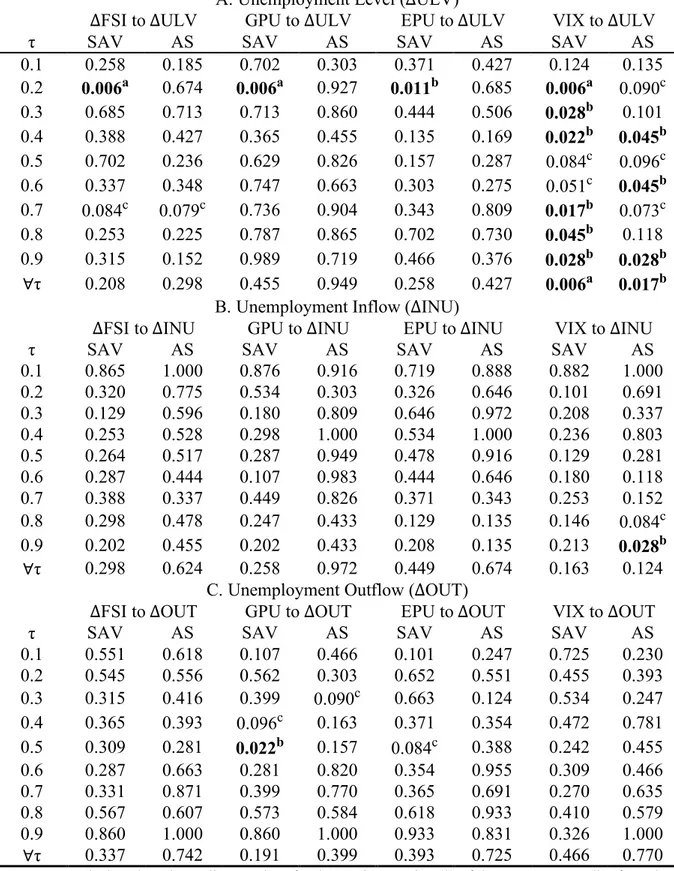
We now analyze the ST test results when we specify nonlinear CAViaR models under 𝐻F in (7).
To highlight the benefits of applying nonlinear models, we compare quantile forecasts for ΔULV, ΔINU, and ΔOUT using linear and nonlinear quantile regression models. We compare the root mean squared error (RMSE) of 120 recursive monthly out-of-sample forecasts of certain quantiles of the distribution. We perform the first forecast on September 1, 2008, and
we increase our in-sample period at each monthly forecast. We consider the following quantiles τ = {0.1, 0.3, 0.5, 0.7, 0.9}, in which we found significant quantile-causality from uncertainty indices to unemployment.
Table 5 presents the RMSE of the recursive quantile forecasts. The linear quantile models outperform the nonlinear CAViaR models for the quantiles τ = {0.3, 0.5} and the upper-tail quantile τ = 0.7. Conversely, the CAViaR models provide a lower RMSE for the tail quantiles τ = 0.1 and τ = 0.9 than linear quantile autoregressive models. Thus, we find evidence that CAViaR models have a better specification for the extreme tail quantiles of unemployment series.
Table 6.A displays the quantile-causality test results for unemployment changes using nonlinear specifications under 𝐻F in Equation (7). There is still causality from ΔFSI to ΔULV at the
quantile τ = 0.7 at the 10% level, but both GPU and EPU do not lead ΔULV at all quantiles. On the other hand, VIX leads ΔULV at all quantiles greater than τ = 0.1, when we apply nonlinear quantile specifications. Therefore, nonlinear quantile models uncover a strong pattern of VIX-ΔULV causality.
Tables 6.B and 6.C show the quantile-causality test results for unemployment inflow and outflow using nonlinear quantile specifications under the null hypothesis. In line with the results displayed in Table 3, we find absence of nonlinear quantile-causality from uncertainty indices to unemployment inflow and outflow.
To highlight the usefulness of our findings, we check whether the observed uncertainty-unemployment causality improves the out-of-sample predictability to uncertainty-unemployment. In-sample predictability of uncertainty does not necessary entail out-of-In-sample forecast improvements. We consider the quantiles with significant uncertainty-unemployment causality τ = {0.1, 0.3, 0.5, 0.7, 0.9}. We perform 120 recursive monthly out-of-sample forecasts on these quantiles, using a QAR(1) model and an enlarged model that includes a past uncertainty index. We perform the first forecast on September 1, 2008, and we increase our in-sample period at each monthly forecast. To compare the forecast models, we employ the modified Diebold and Mariano (1995)’s test of Harvey et al. (1997) and the Clark and West
(2007)’s test of equal forecast accuracy. For both tests, the quantile-forecasts errors of both forecast models are equal under the null hypothesis.
Table 7 illustrates the out-of-sample predictability test results. The observed causality from ΔFSI to ΔULV at upper-tail quantiles does not help improve the predictability to ΔULV. Conversely, the observed GPU-ΔULV nonlinear causal relationship at the lower-tail quantile τ=0.1 improves the out-of-sample predictability to ΔULV, at the 5% level. Further, the Granger-causality from VIX to ΔULV enhances the out-of-sample predictability to ΔULV at the quantiles τ = {0.3, 0.5, 0.7, 0.9}. These results corroborate the nonlinear quantile-causality findings presented in Table 6.A, where the causality from VIX to ΔULV is strong at all quantiles except for the lower-tail quantile of τ=0.1.
Table 7 also shows that lagged values of GPU, EPU, and VIX improve the out-of-sample predictability of ΔINU at the lower-tail quantile τ=0.1, conforming to the quantile-causality outcomes displayed in Table 4.B. Nevertheless, lagged values of ΔFSI do not help predict ΔINU, at the 5% level. Finally, the observed causality from GPU and EPU to ΔOUT is significant to the out-of-sample predictability of ΔOUT at the lower-tail quantiles of τ=0.1 and τ=0.3.
Consistent with Gupta et al. (2018), the impacts of uncertainty depend on the states (quantiles) of the U.S. economy. Further, the effects of uncertainty on U.S. unemployment depend on the uncertainty measure and on the specification of the quantile regression model. We also provide evidence of improvements in out-of-sample predictability of uncertainty to the unemployment level; these findings corroborate the results of Segnon et al. (2018), who showed that uncertainty improves the precision of U.S. GNP growth forecasts. Our findings are also consistent with Caggiano et al. (2014), Jones and Enders (2016), Caggiano et al. (2017a, 2017b), and Chatterjee (2019), among others, who found that the reaction of U.S. unemployment to uncertainty is asymmetric along the business cycle.
5. Conclusion and Policy Implications
Uncertainty affects almost all decisions in an economy. In this paper, we explore how uncertainty influences decisions about hiring and firing in the U.S. labor market. Our findings
indicate that uncertainty leads to positive shocks in the unemployment level, which reaffirms certain results of earlier research (Bloom, 2009; Abaidoo, 2012; Bachmann and Bayer, 2013; Jurado et al., 2015; Baker et al., 2016; Bloom et al., 2018; Mumtaz, 2018). We then break down the unemployment level into inflow that is a result of firing (or quitting on the worker’s side) and outflow that is a result of hiring (or job finding on the worker’s side). We see that uncertainty leads to positive shocks on unemployment inflow, in line with the search and matching model of Schaal (2017), while uncertainty negatively affects U.S. unemployment outflow. As our findings are consistent across different measures of uncertainty, these measures seem to succeed in measuring economic uncertainty about the future in a more general sense. We corroborate the previously documented nonlinear impacts of uncertainty on the unemployment level (Caggiano et al., 2014; Nodari, 2014; Caggiano et al., 2017a, 2017b). In addition, we find that uncertainty and unemployment flows are linearly connected.
Our results corroborate the general predictions from a search and matching framework of how uncertainty affects unemployment and its flows. Specifically, the findings that fluctuations in different types of uncertainty leads to positive shocks in unemployment level, positive shocks to inflow, and negative (but weaker, or more delayed) shocks to outflow are all in line with theory. Further, the finding that the uncertainty-unemployment level relation is nonlinear while the uncertainty-unemployment flows relation is linear is also in line with theory.
Our main policy implication is that government and policymakers should strive for economic stability insofar as possible, if they wish to manage the unemployment level of the economy. The differences in effects we observe across four uncertainty measures indicate that such stability is especially important in the financial sector, which our results show that has the strongest connection to unemployment and its flows, but it is also important in domestic and global economic policy. Reducing the fluctuations in uncertainty will lead to a more stable rate of job separation, because uncertainty leads to positive shocks to unemployment inflow. In addition, uncertainty negatively affects outflow. The level of unemployment at any given time is a positive function of inflow and a negative function of outflow, which means that the heterogeneous linkage between uncertainty and flows induces increases in the unemployment level. Thus, reducing the fluctuations in uncertainty will help control both of the flows in a way that reduces the level of unemployment. This analysis is complicated by the nonlinear relation between uncertainty and unemployment level and, as we demonstrate, becomes much clearer once flows are considered.
Certain authors (e.g. Bloom, 2009; Basu and Bundick, 2017; Caggiano et al., 2017b) recommend designing monetary and fiscal policies that manage fluctuations in uncertainty; our results indicate that such stabilization policies would have positive effects for the labor market as well. However, since monetary and fiscal policy interventions may be ineffective in episodes of heightened uncertainty (Bloom, 2009; Bloom et al., 2018), insofar as these results apply to the labor market, we would caution against reactive policies that counterbalance uncertainty impacts on unemployment. Therefore, implementing more direct employee protection subsidies that are enabled during uncertain times is a possible intervention as long as it is not done reactively. Another way for policymakers to reduce fluctuations in uncertainty is to increase the overall transparency in the regulatory process and to work towards more long-term plans than those that are typically enacted, so that businesses and other economic actors face less uncertainty about their future.
In sum, this paper highlights the importance of using unemployment flow data when analyzing issues related to unemployment, because in doing so we have been able to provide a comprehensive picture of how economic uncertainty relates to unemployment. Furthermore, we have shown that while the relation between uncertainty and the unemployment level is nonlinear, it can be explained through a linear relation between uncertainty and unemployment flows, which in turn are nonlinearly connected to the unemployment level. Our findings are important for policymakers who need to incorporate the uncertainty measures to predict the inflows and outflows to unemployment.
References
Abaidoo, R., 2012. Policy uncertainty, macroeconomic dynamics, and US unemployment conditions. Journal of Applied Business Research 28, 777–789.
Andrews, D.W.K., 1993. Tests for parameter instability and structural change with unknown change point. Econometrica 61, 821–856.
Andrews, D.W.K., Ploberger, W., 1994. Optimal tests when a nuisance parameter is present only under the alternative. Econometrica 62, 1383–1414.
Antonakakis, N., Gupta, R., Andre, C., 2015. Dynamic co-movements between economic political uncertainty and housing market returns. Journal of Real Estate Portfolio Management 21, 53–60.
Bachmann, R., Bayer, C., 2013. ‘Wait-and-See’ business cycles? Journal of Monetary Economics 60, 704–719.
Bachmann, R., Elstner, S., Sims, E.R., 2013. Uncertainty and economic activity: Evidence from business survey data. American Economic Journal: Macroeconomics 5, 217–249.
Baker, S.R., Bloom, N., Davis, S.J., 2016. Measuring economic policy uncertainty. The Quarterly Journal of Economics 131, 1593–1636.
Bao, Y., Lee, T.-H., Saltoglu, B., 2006. Evaluating predictive performance of value-at-risk models in emerging markets: A reality check. Journal of Forecasting 25, 101–128.
Basu, S., Bundick, B., 2017. Uncertainty shocks in a model of effective demand. Econometrica 85, 937–958.
Bernanke, B.S., 1983. Irreversibility, uncertainty, and cyclical investment. The Quarterly Journal of Economics 98, 85–106.
Bloom, N., 2014. Fluctuations in uncertainty. Journal of Economic Perspectives 28, 153–176. Bloom, N., 2009. The impact of uncertainty shocks. Econometrica 77, 623–685.
Bloom, N., Bond, S., Van Reenen, J., 2007. Uncertainty and investment dynamics. Review of Economic Studies 74, 391–415.
Bloom, N., Floetotto, M., Jaimovich, N., Saporta Eksten, I., Terry, S., 2018. Really uncertain business cycles. Econometrica 86, 1031–1065.
Breusch, T.S., 1978. Testing for autocorrelation in dynamic linear models. Australian Economic Papers 17, 334–355.
Broock, W.A., Scheinkman, J.A., Dechert, W.D., LeBaron, B., 1996. A test for independence based on the correlation dimension. Econometric Reviews 15, 197–235.
Caggiano, G., Castelnuovo, E., Figueres, J.M., 2017a. Economic policy uncertainty and unemployment in the United States: A nonlinear approach. Economics Letters 151, 31– 34.
Caggiano, G., Castelnuovo, E., Groshenny, N., 2014. Uncertainty shocks and unemployment dynamics in US recessions. Journal of Monetary Economics 67, 78–92.
Caggiano, G., Castelnuovo, E., Pellegrino, G., 2017b. Estimating the real effects of uncertainty shocks at the Zero Lower Bound. European Economic Review 100, 257–272.
Calcagnini, G., Saltari, E., 2000. Real and financial uncertainty and investment decisions. Journal of Macroeconomics 22, 491–514.
Chatterjee, P., 2019. Asymmetric impact of uncertainty in recessions: Are emerging countries more vulnerable? Studies in Nonlinear Dynamics & Econometrics 23.
Chen, Q., Gerlach, R., Lu, Z., 2012. Bayesian Value-at-Risk and expected shortfall forecasting via the asymmetric Laplace distribution. Computational Statistics and Data Analysis 56, 3498–3516.
Chen, Y.F., Funke, M., 2004. Working time and employment under uncertainty. Studies in Nonlinear Dynamics and Econometrics 8.
Choi, S., 2017. Variability in the effects of uncertainty shocks: New stylized facts from OECD countries. Journal of Macroeconomics 53, 127–144.
Chow, S.C., Cunado, J., Gupta, R., Wong, W.K., 2017. Causal relationships between economic policy uncertainty and housing market returns in China and India: Evidence from linear and nonlinear panel and time series models. Studies in Nonlinear Dynamics and Econometrics 22, 1–15.
Clark, T.E., West, K.D., 2007. Approximately normal tests for equal predictive accuracy in nested models. Journal of Econometrics 138, 291–311.
Cosar, A.K., Guner, N., Tybout, J., 2016. Firm dynamics, job turnover, and wage distributions in an open economy. American Economic Review 106, 625–663.
Davis, S.J., Faberman, R.J., Haltiwanger, J.C., 2013. The establishment-level behavior of vacancies and hiring. Quarterly Journal of Economics 128, 581–622.
Dickey, D.A., Fuller, W.A., 1979. Distribution of the estimators for autoregressive time series with a unit root. Journal of the American Statistical Association 74, 427–431.
Diebold, F.X., Mariano, R.S., 1995. Comparing predictive accuracy. Journal of Business & Economic Statistics 13, 253–263.
Diks, C., Panchenko, V., 2006. A new statistic and practical guidelines for nonparametric Granger causality testing. Journal of Economic Dynamics & Control 30, 1647–1669. Diks, C., Wolski, M., 2016. Nonlinear Granger Causality: Guidelines for Multivariate Analysis.
Journal of Applied Econometrics 31, 1333–1351.
Dixit, A.K., Pindyk, R.S., 1994. Investment Under Uncertainty. Princeton University Press, Princeton NJ.
Elliott, G., Rothenberg, T.J., Stock, J.H., 1996. Efficient tests for an autoregressive unit root. Econometrica 64, 813–836.
Elsby, M.W.L., Hobijn, B., Şahin, A., 2013. Unemployment dynamics in the OECD. Review of Economics and Statistics 95, 530–548.
Engle, R.F., Manganelli, S., 2004. CAViaR: Conditional autoregressive value at risk by regression quantiles. Journal of Business & Economic Statistics 22, 367–381.
Fernández-Villaverde, J., Guerrón-Quintana, P., Kuester, K., Rubio-Ramírez, J., 2015. Fiscal volatility shocks and economic activity. American Economic Review 105, 3352–3384. Gayle, G.-L., Golan, L., Miller, R.A., 2015. Promotion, turnover, and compensation in the
executive labor market. Econometrica 83, 2293–2369.
Ghosal, V., Ye, Y., 2015. Uncertainty and the employment dynamics of small and large businesses. Small Business Economics 44, 529–558.
Godfrey, L.G., 1978. Testing for higher order serial correlation in regression equations when the regressors include lagged dependent variables. Econometrica 46, 1303–1310.
Granger, C.W.J., 1980. Testing for causality: A personal viewpoint. Journal of Economic Dynamics and Control 2, 329–352.
Granger, C.W.J., 1969. Investigating causal relations by econometric models and cross-spectral methods. Econometrica 37, 424–438.
Gupta, R., Ma, J., Risse, M., Wohar, M.E., 2018. Common business cycles and volatilities in US states and MSAs: The role of economic uncertainty. Journal of Macroeconomics 57, 317–337.
Hall, B.J., Liebman, J.B., 1998. Are CEOs really paid like bureaucrats? Quarterly Journal of Economics 113, 653–691.
Hansen, B.E., 1997. Approximate asymptotic p values for structural-change tests. Journal of Business & Economic Statistics 15, 60–67.
Harvey, D., Leybourne, S., Newbold, P., 1997. Testing the equality of prediction mean squared errors. International Journal of Forecasting 13, 281–291.
Hiemstra, C., Jones, J.D., 1994. Testing for linear and nonlinear Granger causality in the stock price-volume relation. Journal of Finance 49, 1639–1664.
Jens, C.E., 2017. Political uncertainty and investment: Causal evidence from US gubernatorial elections. Journal of Financial Economics 124, 563–579.
Jeon, J., Taylor, J.W., 2013. Using CAViaR models with implied volatility for value-at-risk estimation. Journal of Forecasting 32, 62–74.
Jones, P.M., Enders, W., 2016. The asymmetric effects of uncertainty on macroeconomic activity. Macroeconomic Dynamics 20, 1219–1246.
Jurado, K., Ludvigson, S.C., Ng, S., 2015. Measuring uncertainty. American Economic Review 105, 1177–1216.
Koenker, R., Machado, J.A.F., 1999. Goodness of fit and related inference processes for quantile regression. Journal of the American Statistical Association 94, 1296–1310. Koop, G., Potter, S.M., 1999. Dynamic asymmetries in U.S. unemployment. Journal of
Business & Economic Statistics 17, 298–312.
Lagakos, D., Moll, B., Porzio, T., Qian, N., Schoellman, T., 2018. Life cycle wage growth across countries. Journal of Political Economy 126, 797–849.
Economics 82, 20–35.
Lee, T.-H., Yang, W., 2012. Money-income Granger-causality in quantiles, in: Terrell, D., Millimet, D. (Eds.), 30th Anniversary Edition (Advances in Econometrics, Volume 30). Emerald Group Publishing Limited, pp. 383–407.
MacKinnon, J.G., White, H., 1985. Some heteroskedasticity-consistent covariance matrix estimators with improved finite sample properties. Journal of Econometrics 29, 305–325. Morley, J., Piger, J., 2012. The asymmetric business cycle. Review of Economics and Statistics
94, 208–221.
Morley, J., Piger, J., Tien, P.-L., 2013. Reproducing business cycle features: are nonlinear dynamics a proxy for multivariate information? Studies in Nonlinear Dynamics and Econometrics 17, 483–498.
Mortensen, D.T., Pissarides, C.A., 1994. Job creation and job destruction in the theory of unemployment. The Review of Economic Studies 61, 397–415.
Mumtaz, H., 2018. Does uncertainty affect real activity? Evidence from state-level data. Economics Letters 167, 127–130.
Nodari, G., 2014. Financial regulation policy uncertainty and credit spreads in the US. Journal of Macroeconomics 41, 122–132.
Panousi, V., Papanikolaou, D., 2012. Investment, idiosyncratic risk, and ownership. Journal of Finance 67, 1113–1148.
Pastor, L., Veronesi, P., 2013. Political uncertainty and risk premia. Journal of Financial Economics 110, 520–545.
Pastor, L., Veronesi, P., 2012. Uncertainty about government policy and stock prices. Journal of Finance 67, 1219–1264.
Pissarides, C.A., 2000. Equilibrium Unemployment Theory, Second. ed. Cambridge, MA:MIT Press.
Sakov, A., Bickel, P., 2000. An Edgeworth expansion for the m out of n bootstrapped median. Statistics & Probability Letters 49, 217–223.
Schaal, E., 2017. Uncertainty and unemployment. Econometrica 85, 1675–1721.
Scotti, C., 2016. Surprise and uncertainty indexes: Real-time aggregation of real-activity macro-surprises. Journal of Monetary Economics 82, 1–19.
Segnon, M., Gupta, R., Bekiros, S., Wohar, M.E., 2018. Forecasting US GNP growth: The role of uncertainty. Journal of Forecasting 37, 541–559.
Shimer, R., 2012. Reassessing the ins and outs of unemployment. Review of Economic Dynamics 15, 127–148.
Troster, V., 2018. Testing for Granger-causality in quantiles. Econometric Reviews 37, 850– 866.
Troster, V., Shahbaz, M., Uddin, G.S., 2018. Renewable energy, oil prices, and economic activity: A Granger-causality in quantiles analysis. Energy Economics 70, 440–452. Yashiv, E., 2007. Labor search and matching in macroeconomics. European Economic Review
51, 1859–1895.
Yu, P.L.H., Li, W.K., Jin, S., 2010. On some models for value-at-risk. Econometric Reviews 29, 622–641.
Zhang, Y., Wan, G.H., 2004. Liquidity constraint, uncertainty and household consumption in China. Applied Economics 36, 2221–2229.
Tables and Figures Table 1. Descriptive Statistics
Unemployment Uncertainty
ULV INU OUT FSI GPU EPU VIX
Mean 9.04 7.53 7.63 -0.09 4.64 4.70 2.95 Std. Dev. 0.29 0.13 0.10 1.03 0.37 0.37 0.35 Skewness 0.66 0.85 0.47 1.11 0.31 0.15 0.47 Kurtosis -0.71 0.53 -0.07 2.37 -0.52 -0.40 0.07 Jarque-Bera 24.00a 34.75a 9.45a 116.41a 6.81b 2.54 9.86a ADF I(0) -1.68 -1.62 -1.05 -2.23 -4.77a -5.66a -4.24a ADF I(1) -3.20a -18.05a -12.37 a -11.01a -12.40a -13.38a -13.05a ERS I(0) -1.98 -1.82 -1.40 -3.07a -4.75a -5.70a -4.09a ERS I(1) -2.87a -3.24a -2.67a -10.83a -12.26a -12.09a -13.11a Obs. 260 260 260 260 260 260 260
Notes: All variables are transformed to their natural logarithm except for FSI. ADF is the Augmented Dickey-Fuller unit-root test proposed by Dickey and Fuller (1979). ERS is the unit-root test of Elliott et al. (1996). All variables are in level in this table but differenced according to the ADF and ERS test results in subsequent analyses. The notation a and b indicate rejection of the null hypothesis that the series is I(1) at the 1% and 5% significance levels, respectively. The data on unemployment were retrieved from the BLS, Bureau of Labor Statistics, from https://www.bls.gov/webapps/legacy/cpsflowstab.htm. FSI and VIX were retrieved from FRED, Federal Reserve Bank of St. Louis, from https://fred.stlouisfed.org. Data for GPU and EPU are the result of work by Baker et al. (2016) and were retrieved from https://www.policyuncertainty.com.
Table 2. Granger-Causality Tests in Mean and Nonlinearity Tests Panel A. Granger-Causality Tests in Mean
Null hypothesis P-value (F-test) L Breusch-Godfrey test
ΔFSI to ΔULV 0.209 6 0.276 GPU to ΔULV 0.350 6 0.479 EPU to ΔULV 0.323 6 0.128 VIX to ΔULV 0.026b 5 0.077 ΔFSI to ΔINU 0.272 2 0.065 GPU to ΔINU 0.266 2 0.052 EPU to ΔINU 0.086c 5 0.093 VIX to ΔINU 0.003a 5 0.581 ΔFSI to ΔOUT 0.074c 2 0.110 GPU to ΔOUT 0.109 4 0.291 EPU to ΔOUT 0.102 4 0.190 VIX to ΔOUT 0.254 3 0.053
Notes: This table shows the p-values of a Granger-causality test shown in Equations (5)-(6), where the null hypothesis is Granger-non-causality from each uncertainty index to the respective unemployment measure. The notation a, b, and c indicate rejection of the null hypothesis at the 1%, 5%, and 10% significance levels, respectively. L indicates the lag length of the VAR model that minimized the BIC such that the VAR residuals were serially uncorrelated. Breusch-Godfrey test denotes the p-values of the serial correlation test of the residuals proposed by Breusch (1978) and Godfrey (1978). The residuals are uncorrelated under the null hypothesis. The GPU, EPU, and VIX are stationary series in level, and thus they were not differenced.
Panel B. Nonlinearity Tests
VAR BDS (m=2) BDS (m=3) BDS (m=4) SupF AveF ExpF
ΔULV, ΔFSI 0.146 0.503 0.565 0.006a 0.012b 0.008a ΔULV, GPU 0.547 0.996 0.907 0.005a 0.043b 0.005a ΔULV, EPU 0.300 0.659 0.504 0.023b 0.043b 0.021 ΔULV, VIX 0.400 0.841 0.819 0.000a 0.004a 0.000a ΔINU, ΔFSI 0.962 0.600 0.320 0.609 0.539 0.626 ΔINU, GPU 0.785 0.519 0.215 0.029b 0.225 0.081c ΔINU, EPU 0.541 0.134 0.027b 0.000a 0.022b 0.000a ΔINU, VIX 0.877 0.525 0.134 0.000a 0.069c 0.001a ΔOUT, ΔFSI 0.260 0.585 0.946 0.913 0.548 0.718 ΔOUT, GPU 0.183 0.871 0.518 0.092c 0.074c 0.068c ΔOUT, EPU 0.162 0.897 0.500 0.129 0.104 0.101 ΔOUT, VIX 0.152 0.945 0.632 0.701 0.663 0.646
Notes: This table presents the p-values of the BDS test for nonlinearity in the VAR residuals of Broock et al. (1996), where m denotes the dimension. The residuals are i.i.d. under the null hypothesis. The SupF, AveF, and ExpF are the tests of parameter stability of the VAR models proposed by Andrews (1993), Andrews and Ploberger (1994), and Hansen (1997), respectively. The notation a, b, and c denote rejection of the null hypothesis at the 1%, 5%, and 10% significance levels, respectively.
Table 3. Nonlinear and Multivariate Granger-Causality Tests in Mean Panel A. Nonlinear Granger-Causality Tests in Mean
Null hypothesis L P-value (HJ) P-value (DP)
ΔFSI to ΔULV 6 0.643 0.625 GPU to ΔULV 6 0.674 0.659 EPU to ΔULV 6 0.885 0.183 VIX to ΔULV 5 0.909 0.182 ΔFSI to ΔINU 2 0.737 0.342 GPU to ΔINU 2 0.840 0.837 EPU to ΔINU 5 0.626 0.704 VIX to ΔINU 5 0.886 0.802
Notes: This table shows the p-values of the nonlinear causality tests HP and DP of Hiemstra and Jones (1994) and Diks and Panchenko (2006), respectively. We used the lag order that minimized the BIC on the bivariate VAR models. We applied the test on the standardized residuals of the VARs with a bandwidth of 𝜖 = 1.5.
Panel B. Multivariate Granger-Causality Tests in Mean
Null hypothesis P-value (F-test) L
Breusch-Godfrey test P-value (DW)
ΔFSI to ΔULV 0.015b 8 0.171 0.121 GPU to ΔULV 0.471 8 0.171 0.858 EPU to ΔULV 0.519 8 0.171 0.961 VIX to ΔULV 0.078c 8 0.171 0.782 ΔFSI to ΔINU 0.013b 4 0.086 0.327 GPU to ΔINU 0.035b 4 0.086 0.918 EPU to ΔINU 0.362 4 0.086 0.303 VIX to ΔINU 0.001a 4 0.086 0.482 ΔFSI to ΔOUT 0.374 2 0.081 0.517 GPU to ΔOUT 0.117 2 0.081 0.803 EPU to ΔOUT 0.575 2 0.081 0.653 VIX to ΔOUT 0.000a 2 0.081 0.178
Notes: This table presents the p-values of multivariate Granger-causality tests in mean. The F-test is a linear Granger-causality in mean test that is calculated in a multivariate VAR model with an unemployment series and four uncertainty indices. We used the lag order that minimized the BIC on the multivariate VAR models. Breusch-Godfrey test denotes the p-values of the serial correlation test of the residuals proposed by Breusch (1978) and Godfrey (1978). The VAR residuals are serially uncorrelated under the null hypothesis. The notation
a, b, and c denote rejection of the null hypothesis at the 1%, 5%, and 10% significance levels, respectively. DW
test is the multivariate nonlinear causality test of Diks and Wolski (2016) on the standardized residuals of the multivariate VARs. We used a bandwidth parameter of 𝜖 = 1.021 to calculate the p-values of the DW test.
A. Unemployment Level (ΔULV)
ΔFSI to ΔULV GPU to ΔULV EPU to ΔULV VIX to ΔULV
τ L=1 L=2 L=3 L=1 L=2 L=3 L=1 L=2 L=3 L=1 L=2 L=3 0.1 0.311 0.212 0.269 0.113 0.090c 0.179 0.311 0.137 0.198 0.033b 0.033b 0.038b 0.2 0.783 0.840 0.896 0.901 0.877 0.986 0.731 0.892 0.868 0.226 0.429 0.481 0.3 0.863 0.778 0.807 0.887 0.962 0.533 0.396 0.741 0.425 0.212 0.264 0.297 0.4 0.274 0.486 0.623 0.415 0.608 0.373 0.302 0.358 0.292 0.156 0.245 0.203 0.5 0.330 0.684 0.212 0.608 0.769 0.316 0.410 0.524 0.217 0.123 0.410 0.137 0.6 0.783 0.198 0.382 0.939 0.755 0.599 0.910 0.392 0.448 0.377 0.028b 0.170 0.7 0.014b 0.071c 0.099c 0.028b 0.406 0.387 0.033b 0.321 0.392 0.005a 0.042b 0.066c 0.8 0.014b 0.264 0.500 0.057c 0.675 0.929 0.019b 0.722 0.920 0.005a 0.123 0.208 0.9 0.085c 0.137 0.014b 0.552 0.590 0.071c 0.297 0.387 0.047b 0.033b 0.005a 0.014b ∀τ 0.137 0.557 0.278 0.557 0.929 0.608 0.297 0.698 0.382 0.042b 0.057c 0.118
B. Unemployment Inflow (ΔINU)
ΔFSI to ΔINU GPU to ΔINU EPU to ΔINU VIX to ΔINU
τ L=1 L=2 L=3 L=1 L=2 L=3 L=1 L=2 L=3 L=1 L=2 L=3 0.1 0.052c 0.278 0.274 0.052c 0.222 0.241 0.052c 0.208 0.231 0.052c 0.236 0.297 0.2 0.250 0.184 0.137 0.222 0.061c 0.052c 0.222 0.075c 0.085c 0.241 0.146 0.104 0.3 0.274 0.519 0.840 0.217 0.406 0.774 0.212 0.344 0.788 0.222 0.387 0.821 0.4 0.788 0.368 0.642 0.769 0.599 0.722 0.910 0.613 0.750 0.656 0.538 0.788 0.5 0.703 0.231 0.368 0.972 0.495 0.802 0.962 0.439 0.783 0.689 0.156 0.288 0.6 0.849 0.722 0.368 1.000 1.000 0.840 0.972 0.788 0.632 0.420 0.349 0.198 0.7 0.212 0.005a 0.005a 0.311 0.005a 0.005a 0.236 0.005a 0.005a 0.137 0.005a 0.005a 0.8 0.009a 0.198 0.113 0.019b 0.439 0.217 0.009a 0.170 0.104 0.009a 0.160 0.057c 0.9 0.005a 0.184 0.472 0.080c 0.354 0.462 0.009a 0.179 0.179 0.005a 0.080c 0.071c ∀τ 0.278 0.038b 0.009a 0.241 0.042b 0.052c 0.217 0.005a 0.019b 0.189 0.009a 0.005a
C. Unemployment Outflow (ΔOUT)
ΔFSI to ΔOUT GPU to ΔOUT EPU to ΔOUT VIX to ΔOUT
τ L=1 L=2 L=3 L=1 L=2 L=3 L=1 L=2 L=3 L=1 L=2 L=3 0.1 0.009a 0.481 0.132 0.042b 0.481 0.099c 0.009a 0.264 0.099c 0.009a 0.509 0.160 0.2 0.830 0.835 0.906 0.736 0.726 0.811 0.943 0.877 0.991 0.792 0.415 0.392 0.3 0.132 0.104 0.127 0.132 0.080c 0.085c 0.132 0.094c 0.113 0.132 0.080c 0.080c 0.4 0.014b 0.245 0.245 0.014b 0.137 0.170 0.014b 0.302 0.377 0.014b 0.193 0.330 0.5 0.075c 0.052c 0.038b 0.075c 0.047b 0.042b 0.080c 0.137 0.085c 0.075c 0.142 0.066c 0.6 0.137 0.108 0.184 0.184 0.170 0.241 0.259 0.193 0.344 0.278 0.193 0.311 0.7 0.906 0.425 0.080c 0.858 0.420 0.198 0.792 0.552 0.222 0.561 0.618 0.212 0.8 0.283 0.840 0.788 0.250 0.646 0.769 0.349 0.887 0.887 0.472 0.741 0.651 0.9 1.000 0.514 1.000 0.750 0.608 1.000 0.566 0.608 0.991 0.816 0.458 0.462 ∀τ 0.033b 0.099c 0.104 0.038b 0.075c 0.123 0.061c 0.156 0.146 0.085c 0.184 0.123
Notes: These tables show the subsampling p-values for the test in Equation (8) of Granger-non-causality from the four uncertainty measures to changes in the unemployment level (ΔULV) in Table 4.A, in the unemployment inflow (ΔINU) in Table 4.B, and in the unemployment outflow (ΔOUT) in Table 4.C. The notation 𝐿 ∈ {1, 2, 3} indicates the lag length of the quantile autoregressive model under 𝐻F. The notation a, b, and c indicate rejection of 𝐻F at the 1%, 5%, and 10% levels, respectively.
The subsample size used to calculate the test statistic is b= 46. The row “∀τ” shows the subsampling p-values of the test in Equation (8) considering all quantiles of ΔULV, ΔINU, and ΔOUT for Tables 4.A, 4.B, and 4.C, respectively.
RMSE ΔULV ΔINU ΔOUT
τ = 0.1 QAR(1) 0.0381 0.0951 0.0916 QAR(2) 0.0377 0.0897 0.0907 QAR(3) 0.0379 0.0882 0.0901 SAV 0.0346 0.1033 0.1033 AS 0.0343 0.0839 0.0623 τ = 0.3 QAR(1) 0.0301 0.0720 0.0572 QAR(2) 0.0288 0.0672 0.0572 QAR(3) 0.0282 0.0681 0.0564 SAV 0.0340 0.0753 0.0683 AS 0.0336 0.0745 0.0631 τ = 0.5 QAR(1) 0.0279 0.0681 0.0544 QAR(2) 0.0271 0.0644 0.0548 QAR(3) 0.0265 0.0641 0.0543 SAV 0.0327 0.0780 0.0872 AS 0.0323 0.0736 0.0668 τ = 0.7 QAR(1) 0.0319 0.0753 0.0617 QAR(2) 0.0315 0.0715 0.0617 QAR(3) 0.0307 0.0713 0.0612 SAV 0.0325 0.0988 0.0854 AS 0.0325 0.0728 0.0629 τ = 0.9 QAR(1) 0.0472 0.0974 0.0885 QAR(2) 0.0469 0.0948 0.0853 QAR(3) 0.0456 0.0956 0.0857 SAV 0.0332 0.1104 0.1196 AS 0.0346 0.0865 0.0689
Notes: This table shows the root mean squared error (RMSE) of 120 recursive monthly out-of-sample quantile forecasts for ΔULV, ΔINU, and ΔOUT. We consider the quantiles τ={0.1, 0.3, 0.5, 0.7, 0.9}. The first forecast date is September 1, 2008. The models that attained the lowest RMSE are in bold.
A. Unemployment Level (ΔULV)
ΔFSI to ΔULV GPU to ΔULV EPU to ΔULV VIX to ΔULV
τ SAV AS SAV AS SAV AS SAV AS
0.1 0.258 0.185 0.702 0.303 0.371 0.427 0.124 0.135 0.2 0.006a 0.674 0.006a 0.927 0.011b 0.685 0.006a 0.090c 0.3 0.685 0.713 0.713 0.860 0.444 0.506 0.028b 0.101 0.4 0.388 0.427 0.365 0.455 0.135 0.169 0.022b 0.045b 0.5 0.702 0.236 0.629 0.826 0.157 0.287 0.084c 0.096c 0.6 0.337 0.348 0.747 0.663 0.303 0.275 0.051c 0.045b 0.7 0.084c 0.079c 0.736 0.904 0.343 0.809 0.017b 0.073c 0.8 0.253 0.225 0.787 0.865 0.702 0.730 0.045b 0.118 0.9 0.315 0.152 0.989 0.719 0.466 0.376 0.028b 0.028b ∀τ 0.208 0.298 0.455 0.949 0.258 0.427 0.006a 0.017b
B. Unemployment Inflow (ΔINU)
ΔFSI to ΔINU GPU to ΔINU EPU to ΔINU VIX to ΔINU
τ SAV AS SAV AS SAV AS SAV AS
0.1 0.865 1.000 0.876 0.916 0.719 0.888 0.882 1.000 0.2 0.320 0.775 0.534 0.303 0.326 0.646 0.101 0.691 0.3 0.129 0.596 0.180 0.809 0.646 0.972 0.208 0.337 0.4 0.253 0.528 0.298 1.000 0.534 1.000 0.236 0.803 0.5 0.264 0.517 0.287 0.949 0.478 0.916 0.129 0.281 0.6 0.287 0.444 0.107 0.983 0.444 0.646 0.180 0.118 0.7 0.388 0.337 0.449 0.826 0.371 0.343 0.253 0.152 0.8 0.298 0.478 0.247 0.433 0.129 0.135 0.146 0.084c 0.9 0.202 0.455 0.202 0.433 0.208 0.135 0.213 0.028b ∀τ 0.298 0.624 0.258 0.972 0.449 0.674 0.163 0.124
C. Unemployment Outflow (ΔOUT)
ΔFSI to ΔOUT GPU to ΔOUT EPU to ΔOUT VIX to ΔOUT
τ SAV AS SAV AS SAV AS SAV AS
0.1 0.551 0.618 0.107 0.466 0.101 0.247 0.725 0.230 0.2 0.545 0.556 0.562 0.303 0.652 0.551 0.455 0.393 0.3 0.315 0.416 0.399 0.090c 0.663 0.124 0.534 0.247 0.4 0.365 0.393 0.096c 0.163 0.371 0.354 0.472 0.781 0.5 0.309 0.281 0.022b 0.157 0.084c 0.388 0.242 0.455 0.6 0.287 0.663 0.281 0.820 0.354 0.955 0.309 0.466 0.7 0.331 0.871 0.399 0.770 0.365 0.691 0.270 0.635 0.8 0.567 0.607 0.573 0.584 0.618 0.933 0.410 0.579 0.9 0.860 1.000 0.860 1.000 0.933 0.831 0.326 1.000 ∀τ 0.337 0.742 0.191 0.399 0.393 0.725 0.466 0.770
Notes: We calculate the subsampling p-values for the test in Equation (8) of Granger-non-causality from the four uncertainty measures to changes in the unemployment level (ΔULV) in Table 6.A, in the unemployment inflow (ΔINU) in Table 6.B, and in the unemployment outflow (ΔOUT) in Table 6.C. SAV is the symmetric absolute value model of Equation (9). AS is the asymmetric slope model of Equation (10). The notation a, b, and c indicate rejection of 𝐻F at the 1%, 5%, and 10% levels, respectively. The subsample size used to calculate
the test statistic is b = 46. The row “∀τ” shows the subsampling p-values for the test in Equation (8) considering all quantiles of ΔULV, ΔINU, and ΔOUT for Tables 6.A, 6.B, and 6.C, respectively.
τ = 0.1 τ = 0.3 τ = 0.5 τ = 0.7 τ = 0.9
DM CW DM CW DM CW DM CW DM CW
Additional Predictability to ΔULVt
ΔFSIt-1 0.806 0.606 0.848 0.595 0.836 0.633 0.857 0.662 0.878 0.299
GPUt-1 0.000a 0.000a 0.006a 0.000a 0.716 0.247 0.997 0.974 1.000 1.000
EPUt-1 0.000a 0.000a 0.008a 0.001a 0.794 0.374 0.999 0.992 1.000 1.000
VIXt-1 0.422 0.198 0.040b 0.011b 0.016b 0.000a 0.003a 0.000a 0.000a 0.000a Additional Predictability to ΔINUt
ΔFSIt-1 0.692 0.273 0.830 0.565 0.789 0.698 0.479 0.261 0.626 0.228 GPUt-1 0.000a 0.000a 0.996 0.990 0.804 0.662 0.999 0.996 1.000 1.000 EPUt-1 0.005a 0.003a 0.813 0.716 0.550 0.420 0.999 0.996 1.000 1.000
VIXt-1 0.012b 0.007a 0.206 0.147 0.738 0.523 0.438 0.210 0.303 0.125
Additional Predictability to ΔOUTt
ΔFSIt-1 0.917 0.836 0.300 0.213 0.161 0.080 0.746 0.616 0.433 0.354
GPUt-1 0.000a 0.000a 0.034b 0.007a 0.813 0.765 1.000 1.000 1.000 1.000
EPUt-1 0.000a 0.000a 0.100 0.038b 0.945 0.930 1.000 1.000 1.000 1.000
VIXt-1 0.783 0.579 0.914 0.834 0.854 0.822 0.307 0.085c 0.000a 0.000a
Notes: This table displays the p-values of the modified version of the test of Diebold and Mariano (1995) developed by Harvey et al. (1997) (DM) and the test of Clark and West (2007). For both tests, the null hypothesis states that the quantile-forecasts errors of the QAR(1) model and the augmented model including a lagged uncertainty index are equal. The notation a, b, and c indicate rejection of the null hypothesis at the 1%, 5%, and 10% significance levels, respectively. We consider 120 recursive monthly out-of-sample quantile forecasts for ΔULV, ΔINU, and ΔOUT. We consider the quantiles τ={0.1, 0.3, 0.5, 0.7, 0.9}. The first forecast date is September 1, 2008, and we recursively update the sample at each monthly forecast.
Figure 2. Estimated Quantile-Regression Coefficients, β(τ), of the Lagged Uncertainty
Figure 2. (continued)