Attention-Based Bi-Directional Long-Short Term
Memory Network for Earthquake Prediction
MD. HASAN AL BANNA 1, (Graduate Student Member, IEEE), TAPOTOSH GHOSH 1, (Graduate Student Member, IEEE),
MD. JABER AL NAHIAN 1, (Graduate Student Member, IEEE), KAZI ABU TAHER 1,
M. SHAMIM KAISER 2, (Senior Member, IEEE), MUFTI MAHMUD 3, (Senior Member, IEEE),
MOHAMMAD SHAHADAT HOSSAIN 4, (Senior Member, IEEE),
AND KARL ANDERSSON 5, (Senior Member, IEEE)
1Department of Information and Communication Technology, Bangladesh University of Professionals, Dhaka 1216, Bangladesh 2Institute of Information Technology, Jahangirnagar University, Dhaka 1342, Bangladesh
3Department of Computer Science, Nottingham Trent University, Nottingham NG11 8NS, U.K.
4Department of Computer Science and Engineering, University of Chittagong, Chittagong 4331, Bangladesh 5Pervasive and Mobile Computing Laboratory, Luleå University of Technology, 931 87 Skellefteå, Sweden
Corresponding authors: Mufti Mahmud (muftimahmud@gmail.com) and Karl Andersson (karl.andersson@ltu.se)
This work was supported by the Information and Communication Technology Division of the Government of the People’s Republic of Bangladesh under Grant 19FS12048.
ABSTRACT An earthquake is a tremor felt on the surface of the earth created by the movement of the major pieces of its outer shell. Till now, many attempts have been made to forecast earthquakes, which saw some success, but these attempted models are specific to a region. In this paper, an earthquake occurrence and location prediction model is proposed. After reviewing the literature, long short-term memory (LSTM) is found to be a good option for building the model because of its memory-keeping ability. Using the Keras tuner, the best model was selected from candidate models, which are composed of combinations of various LSTM architectures and dense layers. This selected model used seismic indicators from the earthquake catalog of Bangladesh as features to predict earthquakes of the following month. Attention mechanism was added to the LSTM architecture to improve the model’s earthquake occurrence prediction accuracy, which was 74.67%. Additionally, a regression model was built using LSTM and dense layers to predict the earthquake epicenter as a distance from a predefined location, which provided a root mean square error of 1.25.
INDEX TERMS Attention, earthquake, LSTM, location, occurrence.
I. INTRODUCTION
Earthquake is a natural catastrophe, which is occurred due to the impingement of tectonic plates. This leads to the release of a great amount of the earth’s internal energy. These earthquake events normally occur in places, which are on the geographical fault lines and a great number of rocks move against each other [1]. Liquid magma is stored in the core of the earth and it leads to a very high temperature resulting in massive energy. These energies require to be released and fault lines help them escape the core of the earth, which causes a great tremor. This vibration is recognized as an earthquake event.
Earthquakes cause great damage to infrastructures, life and may even lead to another natural catastrophe called The associate editor coordinating the review of this manuscript and approving it for publication was Senthil Kumar .
a tsunami. Around 750,000 people have lost their lives and another 125 million people were greatly affected due to earthquake events that occurred between the years 1998 and 2017. Bangladesh is a small South Asian country (latitude: 20.35◦ N to 26.75◦ N, longitude: 88.03◦ E to 92.75◦ E) having Himalayas and Bay of Bengal on two sides of the country. The earthquakes near Bangladesh are considered in this paper as a case study. The country is situated near the boundary of 3 tectonic plates (Indian, Burmese, and Eurasian) and contains a total of 5 fault lines. This is an active seismic region and ranked 5th for the risk of damage [2] because of its dense population. An earthquake having 7.5 magni-tude on the Richter scale may cause the death of around 88,000 people [3]. It may even cause damage to 72,000 build-ings and a loss of 1,075 million dollars in Dhaka, the capital city of the country. An accurate earthquake magnitude and location prediction system can surely abate these losses. This work is licensed under a Creative Commons Attribution 4.0 License. For more information, see https://creativecommons.org/licenses/by/4.0/
Artificial intelligence (AI), machine learning (ML) and deep learning (DL)-based methods are getting popular in future predictions. An ensemble method was adopted by Zhu et al. [4] in wind speed prediction problem. Mahmud et al. [5] used random forest and LSTM to fore-cast arrivals of tourists. Peng et al. [6] reviewed the appli-cation of DL in biological data mining. Li and Wu [7] predicted market style using clustering approach. Customer churn was predicted by Wang et al. [8] using an ensemble approach. For anomaly detection purposes, AI and DL-based methods show promising results. Anomalies in daily living were detected [9], [10] using a novel ensemble approach by Yahaya et al. [11]. Fabietti et al. [12] adopted neural network in order to detect artifacts in local field poten-tials. Ali et al. [13] reviewed the application of CNN in brain region segmentation. Nahian et al. [14] used LSTM in order to detect fall events and also showed a relation between emotion and falls. A data fusion approach was proposed by Nahiduzzaman et al. [15] to detect fall events. A simple ML-based fall detection approach was proposed by Nahian et al. [16], which used cross-disciplinary features. For disease detection and prediction, DL methods are gain-ing popularity. Noor et al. [17] reviewed the application of DL in detecting neurodegenerative disease. DL methods to detect neurological disorder was reviewed by Noor et al. [18]. Miah et al. [19] compared the performances of ML tech-niques to identify dementia. Additionally, AI and ML have been widely applied to diverse fields for their predictive abilities, which include: biological data mining [20], cyber security [21], earthquake prediction [22], financial predic-tion [23], text analytics [24], [25] and urban planning [26]. This also includes methods to support COVID-19 [27] through analyzing lung images acquired by means of com-puted tomography [28], chest x-ray [29], safeguarding work-ers in workplaces [30], identifying symptoms using fuzzy systems [31], and supporting hospitals using robots [32].
Neural network has widely been used in earthquake prediction. Mignan and Broccardo [33] reviewed the efficacy of neural network in earthquake prediction. Zhang and Wang [34] optimized ANN by embedding genetic algorithm to predict earthquakes. Lin et al. [35] proposed an earthquake magnitude prediction model, which used backpropagation neural network (BPNN). Niksarlioglu and Kulahci [36] showed relations between earthquake and environmental parameters and also proposed an earthquake prediction model using ANN. Particle swarm optimiza-tion (PSO)-BPNN was implemented in earthquake appli-cations by Li and Liu [37]. Berhich et al. [38] adopted an LSTM technique to predict earthquakes. Eight seismic indicators were introduced for earthquake prediction by Panakkat and Adeli [39] in 2007. Most of the existing research works are based on these eight seismic indica-tors [22]. They also showed a performance comparison between radial basis function neural network (RBFNN), BPNN and recurrent neural network (RNN), where RNN showed the best detection probability [40]. Chen et al. [41]
adopted a memorized knowledge approach for image caption-ing uscaption-ing RNN. Amar et al. [42] in 2014 proposed a 3-layered RBFNN and BPNN to predict earthquakes. In case of large earthquake events, RBFNN provided better performance than BPNN. Celik et al. [43] in 2016 used ML classifiers to predict the magnitude of earthquake in Turkey region. They used several parameters of the dataset including the partial correlation and auto correlation of delay and proposed using decision tree (DT), liner regression (LR), rap tree, and multi-layer perceptron (MLP) for prediction purposes.
LSTM [44] was used in earthquake prediction of China region by Wang et al. [45] in 2016. They used dropout layer to reduce overfitting. Softmax function was used for the activation of neurons and RMSprop optimizer was included in the proposed architecture. Cai et al. [46] used RNN with LSTM cells to detect anomaly in the precursory data. Das et al. [47] used historical data of earthquake damages with Naive Bayes classifier and LSTM. Kail et al. [48] pro-posed a combination of LSTM and convolutional neural net-work (CNN) for earthquake prediction. The LSTM cells were modified using CNN. Bhandarkar et al. [49] in 2018 showed a comparison of 2 hidden layered LSTM architecture and 2 hidden layered feed forward neural network (FFNN) in earthquake prediction [50]. The proposed LSTM architecture provided better performance than the FFNN model. Rafiei and Adeli [51] in 2017 proposed a 5 layered neural dynamic classification (NDC) network and neural dynamic optimiza-tion to predict earthquake magnitude and locaoptimiza-tion using 8 seismic indicators. The NDC algorithm uses similar layer architecture as the adaptive neuro fuzzy inference system (ANFIS). A PSO technique was adopted by Zhang et al. [52] in 2014 for earthquake prediction. They used 14 anomalies and reduced dimensional impact through data normalization. The proposed model provided better accuracy and stability than clustering methods.
Narayanakumar and Raja [53] in 2016 suggested using Levenberg Marquardt (LM) neural network and 8 seismic indicators to predict earthquake in Himalayan region. They proposed a 1-hidden layered neural network with purelin and sigmoid activation function. Transfer learning was proposed by Maya and Yu [54] in 2019 to improve the learning pro-cess during earthquake prediction. They improved the per-formance of MLP using a combination of MLP and support vector machine (SVM). They also utilized transfer learning to improve the learning capability of MLP. Asim et al. [55] pre-dicted magnitude of Chile, South California, and Hindukush area using a combination of neural network and support vec-tor regression (SVR), where they used 60 features. They used the maximum relevance and minimum redundancy (mRMR) technique to reduce features and provided input to SVR. The output of the regressor was used as the input of an LM neural network model, which utilized PSO for weight opti-mization. For making earthquake predictions in short finite times, Hidden Markov model-based decision systems can be used. Ren et al. [56] proposed ANFIS for finite-time asyn-chronous control problem investigation. He also investigated
the stabilization and boundedness problem of the Markovian neural network [57]. For the short-term prediction of time-series, DL and ML are commonly used. Huang and Kuo [58] used deep CNN for forecasting photovoltaic power, where a short-term prediction was considered. He also [59] proposed to use a combination of Variational Mode Decomposition, CNN, and Gated Recurrent Unit (GRU) algorithms for the prediction of the price of electricity. For the forecasting of COVID-19 cases, a combination of CNN and GRU was used by him. [60]. Shen et al. [61] proposed to use CNN and compared it with GRU-based models for the forecasting of electricity loads.
Since earthquakes show hidden repetitive behavior, a model, which can realize long-term dependencies can be helpful in revealing patterns. LSTM models have some capabilities, but they fail for long sequences. Attention mech-anism can help to overcome these limitations. Ye et al. [62] used Attention Generative Adversarial Network for object transfiguration. Li et al. [63] proposed an attention-based approach to achieve improvement in user attribute classi-fication. In this work, an attention-based LSTM approach for predicting earthquake occurrences was introduced. An LSTM-based location prediction model is also proposed. A large number of inter-disciplinary time-series features for the above-mentioned research problem were explored here. The main contributions of this paper are as follows:
• Establishing an effective attention-LSTM-based archi-tecture for earthquake occurrence and location predic-tion prior to each month. To the best of the author’s knowledge, attention was never been used for earth-quake prediction studies. Exploring this area, good per-formance was achieved in this study.
• Explored G-R seismic indicators as well as more than 7,700 inter-disciplinary time-series features for finding the best feature set. The knowledge of the best feature set can help to eliminate the exploration of the under-performing feature set for future researches.
• Compared the proposed research work with recent earth-quake prediction studies. The comparison with different studies provided an indication of the superiority of the proposed model.
• Combined the earthquake occurrence prediction model with the epicenter location prediction model to provide an overall prediction of future earthquakes.
In the next section, the attention mechanism will be described. Methodology will be discussed in sectionIIIand section IVwill contain the result analysis. The concluding remarks will be presented in sectionV.
II. ATTENTION MECHANISM
The concept of attention was introduced by
Bahdanau et al. [64] in 2015 for machine translation. Though this concept was primarily built for natural language pro-cessing problems, it can be used for other ML fields as well [14]. While dealing with a long sequence of inputs, the performance of LSTM models deteriorates along with
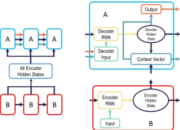
FIGURE 1. The architecture of attention mechanism. There are two parts in attention architecture, which are the encoder part and the decoder part. The blocks of encoder parts are represented by red, and the decoder blocks are represented by cyan. The encoder RNN takes input from the previous encoder hidden states, where the decoder RNN takes input from the decoder input, and the previous decoder hidden states. The decoder input uses the output of the previous context vector and the overall output. The context vector uses encoder hidden states for generating the context for overall output.
the increasing sequence length as giving focus to the whole sequence is difficult. With LSTM, giving focus to a specific portion is also not possible. Attention can help in achieving these goals. If X1, X2, . . . ., XT are considered as the input
sequence and yi as an output sequence at time i, then the
conditional probability of an output event can be calculated as Eq. (1).
P(yi|y1, . . . , yi−1) = g(yi−1, si, ci) (1)
Here, si is the hidden state, which can be calculated
using Eq. (2).
si= f(si−1, yi−1, ci) (2)
Here, ci is the context vector that determines how much
attention is given to each portion of the sequence to calculate the output. It depends on the annotations (h1, h2, . . . .hTx),
where hi have information about the whole sequence with
emphasis on some part surrounding ith position. ci can be
calculated using Eq. (3).
ci= Tx X
j=1
αijhj (3)
Here,αijis the weights that is multiplied with each portion
of the sequence, which is calculated using softmax operation. This is mathematically represented as Eq. (4).
αij=
exp(eij)
PTx
k=1exp(eik)
(4) Here, eijis the alignment of the model, which depends on
si−1, and hj. It is calculated using an FFNN, which trains
automatically while the whole model trains. With these oper-ations, each output is calculated with the weighted sum of the
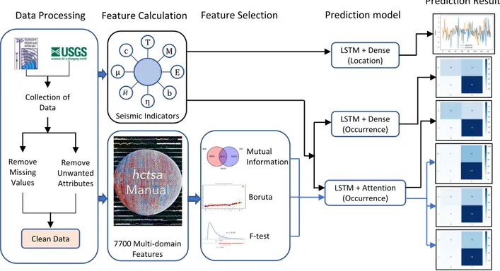
FIGURE 2. The overall methodology of the paper is depicted in the figure. In the data processing portion, the collected data from the USGS and Bangladesh Meteorology Department was cleaned from which the seismic indicators were calculated. HCTSA library was used for calculating the multi-domain features from where the feature selection algorithms were used to select the best features. Different prediction models were created with the combination of LSTM and dense layers for the prediction of occurrence and location of an earthquake. Introduction of attention mechanism improved the performance of the occurrence prediction model. Finally, the models were tested and compared based on their performance.
input sequence, where the weights are elements of the context vector. Fig.1depicts the overall attention mechanism.
III. METHODOLOGY
For this study, data was collected from two sources and preprocessed duly. Then 8 seismic indicators were calculated from the dataset. The proposed attention-based LSTM model was used to predict the occurrence of the earthquake. The analysis pipeline is shown in Fig. 2 and the detailed method-ology is discussed below.
A. DATASET COLLECTION
As a case study, earthquakes around Bangladesh were con-sidered. Earthquake catalog from Bangladesh meteorological department of the year 1950 to 2019 was collected along with earthquake catalog from the United States geological survey (USGS) of the same time duration [65]. There are six features in the meteorological department dataset, which are-date, time, longitude, latitude, magnitude, and depth. In the USGS dataset, there are seventeen more attributes like-type of the disaster, update date, earthquake id, depth error, and so on. Only the magnitude type feature was used from that dataset. Other features were dropped. For finding the magnitude of an earthquake, different scales are used. Therefore, the mag-nitude type parameter was used to convert the dataset into a particular scale. The Richter scale was used as the default magnitude scale. The data of 18.11◦N to 27.11◦N latitude and 87.19◦E to 95.36◦E longitude was collected. This covers
the area around Bangladesh. From here 1,764 records of earthquakes were found. These records were used to calculate the features for prediction.
B. DATASET PREPROCESSING
Preprocessing of data is a very important step for achieving good prediction. For finding out any inconsistency in the earthquake catalog, the data of the meteorological depart-ment and USGS was cross-checked. The missing values were removed and all the magnitudes were converted to the Richter scale. The date, time, longitude, latitude, magnitude, mag-nitude type, and depth parameter were kept for feature cal-culation. The foreshocks and the aftershocks were removed from the dataset and 8 features were calculated based on the mainshocks, which are called the seismic indicators.
C. SEISMIC FEATURE CALCULATION
Here, features specific to the earthquake researches were calculated. Adeli and Panakkat [39] used 8 seismicity indi-cators, which are b-value (b), mean square deviation (MSD), magnitude deficit (MD), elapsed days (ED), mean magnitude (MM ), rate of the square root of energy released (RSRER), mean time between characteristic events (MTBCE), and coef-ficient of variation from mean time (CVFMT ) for earthquake prediction, which were later adopted by many researchers. We, therefore, calculated these features for this research as well. The 8 seismicity indicators were calculated on monthly
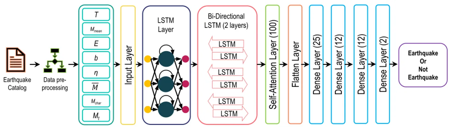
FIGURE 3. The proposed earthquake occurrence prediction model. It is a combination of LSTM layer, bi-directional layers, attention layer, and dense layers.
basis considering the previous 50 events in the calculation. The 8 seismicity indicators are discussed as follows:
1) ELAPSED DAYS (ED)
This represents the time passed over the last n number of earthquake events when the magnitude was greater than a specific value. It is represented by the following equation.
ED = tn− t1 (5)
Here, the time of occurrence of the nthvalue is represented as tnand 1stvalue is represented as t1. In this case, the value
of n was selected as 50. When the ED is small, it means that there was more earthquake leading to that month.
2) MEAN MAGNITUDE (MM)
Mean magnitude is the mean of the n events in Richter scale. This can be formulated as the following equation.
MM = P Mi
n (6)
Here, Miis the magnitude of each event.
3) RATE OF SQUARE ROOT OF SEISMIC ENERGY (RSRER)
Energy (E) of an earthquake can be calculated with the following formula corresponding to the Richter scale mag-nitude, where M is the magnitude of the earthquake.
E =10(11.8+1.5M)ergs (7)
RSRERcan be calculated as the following equation.
RSRER = P E
1/2
ED (8)
4) B-VALUE (b)
This is the slope of log of the frequency of earthquake with respect to magnitude curve. From the Gutenberg-Richter (G-R) inverse power law,
log10N = a − bM (9) Here, a, b are constants, and N is the number of events with magnitude greater or equal to M . The value of a can be
calculated as the following equation.
a = P log10Ni+ bMi
n (10)
Here, Miis the ithmagnitude and Niis the number of events
with magnitude Mior greater. b-value can be calculated as the
following equation.
b = (nP Milog10Ni) −P MiP log10Ni)
((P Mi)2− nP Mi2)
(11)
5) MEAN SQUARE DEVIATION (MSD)
This is the sum of the mean square deviation from the G-R line. The higher value of this parameter represents inconsis-tency from the G-R inverse power law. This can be calculated as the following equation.
MSD =P (log10Ni−(a − bMi)
2
(n − 1) (12)
6) MAGNITUDE DEFICIT (MD)
This is the residual of the maximum magnitude observed in n events and the largest magnitude based on G-R law. This can be represented as the following equation.
MD = Mmaximum observed− Mmaximum expected (13)
Mmaximum expected can be calculated as the following
equation.
Mmaximum expected = a/b (14) 7) MEAN TIME BETWEEN CHARACTERISTIC
EVENTS (MTBCE )
From the elastic rebound hypothesis [66], earthquakes with high magnitude repeats after some time. This phenomenon is calculated using this feature. The earthquakes between mag-nitude 7 and 7.5 are selected as characteristic earthquakes. The value of MTBCE can be calculated as the following equation.
MTBCE = P (ti characteristics) ncharacteristics
(15) Here, ti characteristicsis the time between two characteristic
8) COEFFICIENT OF VARIATION FROM MEAN TIME (CVFMT )
This value represents the closeness of the characteristic dis-tribution and the magnitude disdis-tribution. It can be mathemat-ically represented as the following equation.
CVFMT=standard deviation of the observed times MTBCE (16)
For this research, 495 time-series sequences were calcu-lated, which were split into 70% (345) and 30% (150) ratios for the training and testing set. The testing portion of the data was kept aside and was not revealed to the training process. Further, 7,700 multi-domain features were calcu-lated using highly comparative time series analysis (HCTSA) library, using a sequence of 50 earthquake magnitude as a time-series [67].
D. SYSTEM CONFIGURATION
The Kaggle kernel was used as a platform to run the codes for the experiments in this study. It provides 4 CPU cores, 16 Gigabytes of RAM, and NVIDIA Tesla P100 GPU. The earthquake occurrence prediction model and the location pre-diction model were implemented in python language. The Keras, tuner, Scikit-learn, NumPy, pandas, statsmodels, and BorutaPy libraries were used for the model building, feature calculation, and model comparisons.
E. EARTHQUAKE OCCURRENCE PREDICTION MODEL
Fig. 3 shows the proposed earthquake occurrence prediction model architecture. In search of the final model, initially, the aim was to find the best combinations of LSTM and dense layers for the earthquake occurrence prediction model. For achieving this goal, the Keras tuner library was used. This library helps to find the best models with different combina-tions. For tuning, the objective was to maximize the validation accuracy. For each of the variations, 10 trials were used to get a stable result. Each model was trained for 1000 epochs and the best model was adopted for the earthquake magnitude prediction model.
After this tuning process, the best model was found to have 200 neurons for the initial LSTM layer, 2 bi-directional LSTM layers with 100 and 50 neurons respectively, a flatten layer, a dense layer with 25 neurons, two dense layers with 12 neurons each, and finally a dense layer with 2 neurons, which works as the output layer. All the layers were trainable and the tanh activation function was used by all the layers except the final layer. Since it is a deep model, overfitting can be an issue. Therefore, L1 and L2 regularization was used for all the LSTM and bi-directional layers. This model is used as a base model for the earthquake occurrence prediction process. The calculated feature set was used to train the model for 10,000 epochs and tested it with the testing set. The learning rate was set to 0.01.
LSTM was developed to eliminate gradient vanishing and gradient exploding problems so that it could be applied across different domains and considered in situations, where the distance between the present and previous knowledge is high.
Three gates make up LSTM cells-an input gate, a forget gate, and an output gate, along with cell state. The input gate determines the necessary information needed to be inserted, and the output gate chooses the subsequent hidden state infor-mation, while forget gate erases the unrelated information. In this work, the previously mentioned 8 seismic features was considered as current input to the LSTM. Thus, the input can be defined as, xt = b − value MSD MD ED MM RSRER MTBCE CVFMT (17)
At first, current inputs were passed through the forget gate along with the previous hidden state information, ht−1. Then
the outcome of the forget gate became
ft =σ(Wf ×[ht−1, xt] + bf) (18)
where, Wf represents the forget gate weights and bf
repre-sents the bias of the forget gate. The input gate determines, which information needs to be updated in the cell state, where the cell state is the memory of the LSTM cell. Sigmoid function and tanh function are used to process the current input and hidden state information and decide modification of the cell state. The output of the sigmoid and tanh function can be obtained as
follows-The output of the sigmoid function,
it =σ(Wi×[ht−1, xt] + bi) (19)
The output of the tanh function, ˜
Ct = tanh(WC×[ht−1, xt] + bC) (20)
Here, Wiand WCare the weights of the input gate and cell
state, and bi and bC are the biases of the input gate and the
cell state, respectively.
A point-wise multiplication is performed to multiply the output from the forget gate and added it with the output from the input gate in order to update the cell’s state. If previous state information is Ct−1and the current state information is
Ct, then,
Ct = ft × Ct−1+ it × ˜Ct (21)
The output gate determines the next hidden state informa-tion according to the following equainforma-tions:
ot =σ(Wo×[ht−1, xt] + bo) (22)
ht = ot× tanh(Ct) (23)
Here, ot is the sigmoid output, ht is the output, Wois the
weights, and bois the bias of the output gate. The output ht
was then fed into the attention layer for further processing. The choice of attention mechanism for this work was the
FIGURE 4. The proposed location prediction model. This model is made with a combination of an LSTM layer, bi-directional layers, and dense layers. The attention mechanism is not used for this model.
Luong attention or the multiplicative attention. This mecha-nism was chosen because it runs faster than additive attention. The attention layer was put before the flatten layer and the attention width was set to 20 previous inputs. L1 and L2 reg-ularization was used for this layer as well. After training this model for 10,000 epochs, a significant improvement was observed in the performance of the model.
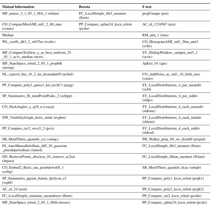
Next, the model was compared with the recent earthquake prediction researches. This model showed impressive results against these models. For investigating the impact of the multi-domain time-series features, 7,700 features were cal-culated, which were normalized so that the proposed model can perform better and have better convergence. Then, dif-ferent feature selection algorithms were used such as mutual information [68], ANOVA F-test [69], and Boruta [70]. Here, 20 best features were selected using mutual information and ANOVA F-test feature selection. Only 2 features were found as important in Boruta feature selection as this algorithm selects only the relevant features. A list of selected features by mutual information, Boruta, and F-test is provided in Table1. Then the proposed attention-LSTM architecture was used for earthquake occurrence prediction using these selected features.
F. EARTHQUAKE LOCATION PREDICTION MODEL
For the prediction of location, a different model was used, which is shown in Fig. 4. The exact longitude and latitude of the earthquake epicenter are not predicted, but the distance from Dhaka city to the origin of the epicenter is predicted. Since the impact of an earthquake does not limit to a small place, rather it expands to a large area, therefore, this pre-diction is enough to find the affected area. Using Campbell’s equation [71], the distance between two points on the earth can be calculated. This can be mathematically calculated using Eq. (24).
D =68.9722 · 0 (24)
Here,0 = [cos−1{(sin a)(sin b) + (cos a)(cos b)(cos P)}] with a and b are the latitude of the first and second point,
respectively, and P is the longitude difference between the two concerned points. With this formula, the distance is calculated in miles which are then converted to kilometers. For Dhaka city, the longitude is 23.81◦N and the longitude is 90.4125◦E. From this point, all the distances are calculated. For the location prediction model, the best model with Keras tuner had an LSTM layer with 200 neurons, two bi-directional LSTM layers with 100 and 50 neurons, a flat-ten layer, and two dense layers with 25 and 12 neurons. Since it was a regression model, the output layer was a dense layer with only 1 neuron and no activation function. The optimization criteria for the tuner was the minimization of validation loss. All the layers, except the output layer, had a tanh activation function. This model was trained for 10,000 epochs as well. Then the mean squared error (MSE) and RMSE was calculated to evaluate the performance of this model.
IV. RESULT ANALYSIS
A. RESULTS OF EARTHQUAKE OCCURRENCE PREDICTION
At first, the performance of the LSTM model was evaluated. After training the model for 10,000 epochs, it was tested for unseen data. Fig. 5 shows the confusion matrix and ROC curve of the LSTM model.
The learning rate was set to 0.01 after trying a wide number of learning rates. Since there are no rules for setting a perfect learning rate, exploring different learning rates is a good option to find the best one. Table2provides an overview of the change in accuracy as learning rate changes. Learning rate 0.01 provided the best result, where learning rate 0.001 and 0.1 gave the worst accuracy. A learning rate of 0.03 provided an accuracy of 0.6934, which was the closest to the achieved accuracy by a learning rate of 0.01 in all the trials. However, the model was trained for 10,000 epochs in all the cases.
In the confusion matrix of Fig. 5 (a), the occurrence of an earthquake is represented as 1 and non-occurrence as 0. From the confusion matrix, the LSTM model can give 106 predic-tions correctly of the 150 events. There were 33 cases, where the model predicted events like earthquakes, but no
earth-TABLE 1. The selected features by the feature selection algorithms from the 7,700 features.
TABLE 2. Change in accuracy depending on the choice of learning rate.
quakes were observed. Of the tested samples 11 earthquakes were not predicted by the model. The ROC curve in Fig. 5 (b) shows that the model can classify both the earthquake and non-earthquake events though the percentage is not really high. The area under the ROC curve is 0.66, which indicates
TABLE 3.Performance of LSTM model.
that this model on average performs correctly for 66% of the cases. Table3shows the detailed results for this model.
The sensitivity (Sn), specificity (Sp), positive predictive
FIGURE 5. (a) Confusion matrix of the LSTM model. It correctly classified 80 out of 91 earthquake occurrences. It provided 33 false alarms in earthquake occurrence prediction. (b) ROC curve of the proposed model. It provided an AUC of 0.660.
FIGURE 6. Impact of attention mechanism in the case of training time after adding with LSTM. Attention-LSTM required only 2.64s more time to train than LSTM after 100 epochs which is very low compared to the improvement of accuracy.
as well. The Snof this model is 0.8791, which is high. This
indicates that the model works very well for positive samples. On the other hand, the Spis 0.4407, which is very low
indicat-ing the false alarms. If the Spof the model can be improved,
a more suitable model can be obtained. The accuracy,
P1, and P0are around 70% mark. But since the false-negative predictions are high, the area under the curve (AUC) param-eter is low for this model.
For time-series data, instead of focusing on the last event, the focus should be on the previous sequences as well. This can be successfully achieved by the use of an atten-tion mechanism, which creates a feature vector for each output. With this mechanism, the proposed model’s perfor-mance can be significantly improved, which is evident in the performed experiments. The attention mechanism required 22.368 seconds, whereas the LSTM needed 19.728 seconds to train for 100 epochs. Therefore, the overall training time for the attention-based model was only 2 minutes and 24 seconds greater than the LSTM model, which did not have an atten-tion mechanism. This should not be a major concern in the
TABLE 4.Performance of attention-based LSTM model.
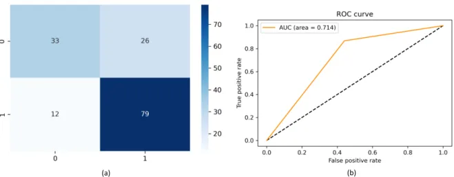
case of earthquake detection as the prediction is made for the following month. Fig. 6 illustrates the comparison of the required training time of the proposed attention-LSTM model and an LSTM model without the attention mechanism. The confusion matrix and the ROC curve of this model have been illustrated in Fig. 7. The attention-based model can rightly predict 112 samples out of the 150 samples. This model’s false positive predictions have been reduced to 26 than the LSTM model (33). The false-negative prediction has increased a bit. The ROC curve is better for this model, which results in a better AUC score. For this model, AUC is 0.714, which is much better than the previous model.
Table 4 shows the detailed result for this model. Here, the specificity of the model is higher than the LSTM model. This means that this model will show a fewer amount of false alarms than the LSTM model. The P1 and P0 value for this model has increased. The accuracy for this model is 74.667%. Therefore, it can be said that this model is much better performing than the previous model.
Next, the multi-domain features were used to train the proposed attention-based architecture to justify the use of seismic indicators as a feature for this region. The mutual information algorithm selected the top 20 features from the pool of 7,700 features. Then these features were used to train
FIGURE 7. (a) Confusion matrix of the proposed attention-based model. It correctly classified 79 out of 91 earthquake events where it provided 26 false alarms in earthquake occurrence prediction. (b) ROC curve of the proposed model. It provided an AUC of 0.714.
FIGURE 8. (a) Confusion matrix of Narayanakumar’s LM model. It correctly classified 54 out of 91 earthquake events. (b) Confusion matrix of an LSTM model by Bhandarkar et al. It has better sensitivity but false alarm is too high. (c) Confusion matrix of the proposed architecture by Aslam et al. It predicted 133 out of 150 events as eartquake which contains a large number of false alarms. (d) Confusion matrix by the proposed model of Wang et al. It correctly classified 57 out of 91 earthquake events.
and test using the proposed attention-LSTM architecture. The accuracy of this model is 0.7067, but the problem with this model is its biasness towards earthquake events. This model predicted 148 out of 150 samples as an earthquake. This means that in most cases, this model just produces a positive prediction.
Boruta feature selection technique selects the highly related as well as loosely related features. Among the 7,700 features, a good number of features were expected to be selected. However, only 2 features were selected by this algorithm. Using these features, the proposed architecture was trained and tested. This pipeline achieved 72% accuracy,
TABLE 5. Performance of the proposed attention-LSTM model and feature reduction techniques in earthquake occurrence prediction that used interdisciplinary time-series features.
where sensitivity and specificity were 0.9427 and 0.2173, respectively. So, this pipeline predicted almost every event as an earthquake but with high false alarms.
With F-test, the top 20 features were selected, with whom the proposed attention-based model was trained. This model achieved an accuracy of 70.67%. The sensitivity of the model was 0.9423, which is very high and means that the model performed very well for positive samples. On the other hand, the specificity of this model was 0.1739. It is very low and indicates lots of false alarms. The negative predictive value is 0.5714, which also indicates that the model performs poorly for non-earthquake events. Table5shows the detailed results of the three feature selection technique-based models. Several recent earthquake prediction models were tested and compared with the proposed model using the data of the study area. The proposed LM model by Narayanakumar et al. had only three layers. The hidden layer had 12 neurons, which used tanh (tan sigmoid) as an activation function. The confusion matrix for this model is presented in Fig. 8 (a). From the confusion matrix, the model can successfully predict 92 out of 150 samples, leading to an accuracy of 61.87%. This model predicted 37 samples as non-earthquake, though they were earthquake events. This means that this model shows biasness towards negative samples.
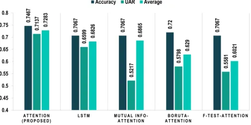
FIGURE 9. Performance comparison of the proposed model with models proposed by Wang et al., Aslam et al., Bhandarkar et al., and
Narayanakumar et al.The proposed architecture achieved better performance in terms of accuracy and UAR than all the above mentioned models in earthquake occurrence prediction.
Bhandarkar et al. [49] proposed an architecture with two LSTM layers having 40 neurons each and tanh activation function. A dropout was also used between these layers, Ada-grad optimizer with an initial learning rate of 7 was adopted in this model. After training it for 10,000 epochs with the data of the study area in consideration, this model achieved 58.67% accuracy, which is much lower than the proposed architecture. This model also provided a large number of false alarms. Fig. 8 (b) illustrates the confusion matrix of the proposed model by Bhandarkar et al.
Aslam et al. [72] proposed an ANN-based architec-ture, which consists of two fully connected layers having 50 neurons and sigmoid activation function. The model was trained using an RMSprop optimizer. This model achieved 61.34% accuracy. But it almost predicted all the samples as earthquake events. Fig. 8 (c) provides the confusion matrix of this model. Wang et al. [45] proposed an architecture with one LSTM layer and two dense layers with 256 and 64 neurons in each. The model was trained with the same configuration of the proposed model. It provided an accuracy of 54.67%, which is lower than the proposed architecture. Fig. 8 (d) pro-vides the confusion matrix of this model.
Fig. 9 shows a comparison of the proposed model with the existing models. The proposed outperformed all the models in the case of accuracy, UAR, and the average of Sn, Sp,
P0, and P1 in earthquake prediction of the selected region. The second-best model in terms of these criteria was the LM-based model by Narayanakumar et al.
In terms of accuracy, the proposed model is 13.34% bet-ter than the LM model. The model proposed by Aslam et
al.also achieved same accuracy as the model proposed by Narayanakumar et al. While on UAR, the proposed model is nearly 10% better. This is a very significant performance difference. The average of Sn, Sp, P0, and P1 is 0.616 for the LM model, which is 11.23% less than the proposed one. Therefore, this can be said that the attention-based LSTM model is much better performing than their model.
Fig. 10 shows the comparison of the proposed seismic indicators-based attention model with multi-domain feature-based models and the initial LSTM model in terms of accu-racy, UAR, and the average of Sn, Sp, P0, and P1, where
the proposed model performed best. In terms of accuracy, the attention model with Boruta feature selection achieved 72% accuracy. The proposed model obtained an accuracy of 74.67%, which is 2.67% better than the closest performing model. The UAR is an average of Snand Sp. For the proposed
model, UAR is 0.7137, which is 5.38% better than the LSTM without attention. The mutual information-based model has an average performance of 0.6865, which is 4.18% lower than the proposed model.
The performance of ML classifiers were also evaluated for earthquake prediction in the Bangladesh region. In Fig. 11, the proposed model was compared with ML-based earth-quake prediction models. It is observed that among the ML algorithms, the proposed model stands out as well. Of the ML algorithms, the RF algorithm shows the best performance
FIGURE 10. Comparison of the proposed earthquake prediction model with the LSTM model and the multi-domain feature models. The proposed model with 8 seismic indicators achieved better accuracy, sensitivity, and specificity than other architectures in earthquake occurrence prediction.
FIGURE 11. Comparison of the proposed models with the ML-based models. RF classifier achieved the best performance among the ML classifiers but could not perform better than the proposed model in earthquake occurrence prediction.
but falls way behind the proposed model in terms of all the metrics. The LR classifier performs the worst for earthquake occurrence prediction. The accuracy of the proposed model is 14% better than the second-best model, while the UAR of the proposed model is 10.14% better. The average is also 11.39% better. This means that the proposed model outperforms the ML classifiers.
From the comparison with the different feature selection techniques, it can be concluded that the selected feature set in the proposed model is the best performing set. Now from the comparison with the ML-classifiers and the recently pro-posed earthquake models, it is evident that for this region, the attention-based LSTM model is the best performing classifier.
B. RESULTS OF EARTHQUAKE LOCATION PREDICTION
The earthquake location prediction process is a distance pre-diction from the center of Dhaka city for this paper. The longi-tude and latilongi-tude of the highest earthquake of a month are used to calculate the distance. Usually, the impact of an earthquake is similar for several hundred kilometers. Since Dhaka is the capital of Bangladesh and most of the important
infrastruc-tures are situated in this city, the distance calculation from this city seemed realistic. MSE and RMSE were used for calcu-lating the performance of this model. The location prediction model is not attention-based as it does not improve the per-formance of the LSTM architecture. Therefore, the attention layer was dropped as it adds complexity to the model. The regression model was trained for 10,000 epochs and tested with a separate 150 samples. Fig. 12 shows the predicted and the actual locations of the earthquakes. Here, it is seen that the actual location is represented using a blue line and the predicted location is predicted using an orange line. It is evident that when the samples are near Dhaka city, the model can predict them well as they match the expected line. But when the distance is very far from the center of the city, the model seems to produce fewer convincing results. For this model, the MSE is 1.5579 and RMSE is 1.24818. The values of these parameters are convincing for earthquake location prediction.
FIGURE 12. Analysis of location prediction result. The predicted location is almost in line with the expected location. However, the proposed architecture failed to predict the location of a seismic event in the case of outliers.
Here, in the green box, the expected and the predicted distance are almost the same. Therefore, it can be said that in
these positions, the distance prediction is perfect. However, in the red boxed areas, peaks can be seen in the distances. These peaks are rare events and very difficult to predict. These peaks are usually considered outliers in the model. But the proposed model can predict some of the peaks. Another significance of this phenomenon is that when the distance is very far away from the center, the model cannot perform well. But the earthquakes which are far from the city are not very important as the earthquake energy declines with distance. Therefore, the proposed model can be used for the location prediction purpose as well.
V. CONCLUSION
The earth is blessed with lots of gifts, which makes life possi-ble to exist. However, natural calamities tear apart the human civilization in a glimpse of an eye. Lots of empires have vanished in destructive natural events. Earthquake is such an event, which can not only demolish infrastructures but also be the cause of millions of deaths. The study area of this paper has faced major earthquakes in the past and has a great chance of witnessing a major one in the near future. The problem with an earthquake is that these events do not show any signs before the occurrence. Precursors are not determined by earthquake researchers. Therefore, a prediction process for earthquakes has become a need of great interest.
Here, historical data of earthquakes in Bangladesh was collected, which can be represented as time-series. Review-ing researches for time-series analysis, it was found that among the existing algorithms, LSTM is a great tool for this purpose. But it faces difficulties in working with long sequences. Therefore, the attention mechanism was appended with the LSTM model that provided the best-found result (74.67% accuracy) in occurrence prediction using 8 seismic indicators. Several ML algorithms were tested in this regard. The proposed model provided significantly better perfor-mance than these architectures.
The inter-disciplinary features were explored for improve-ment from the seismic indicator’s feature set, but no promis-ing improvements were found. The earthquake location was also being predicted with a very good RMSE (1.5579) using LSTM and dense layers. The goal of this research was to build a complete earthquake prediction system and find the best possible set of features for this purpose. The proposed mod-els showed good results for the study region, but improve-ment in accuracy can make the model more suitable. This model predicts the earthquake of the following month, but the exact time of occurrence is not provided. In the future, through adopting these improvements, earthquake prediction researches can be accelerated.
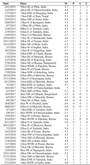
APPENDIX
Here, the prediction of the earthquake events are presented by the proposed model from the year 2015 to February 2019. The date, place, and magnitude along with the prediction are added. Table6shows the predictions.
TABLE 6.Performance of the proposed model in the case of latest earthquake events occurred in the study region.
The tremors with magnitude 4.7 or greater were consid-ered as earthquakes. There are 51 events between 2015 and February 2019, where 40 out of the 51 events were predicted correctly by the proposed model. That means that the model is more than 78% accurate in this time span. The place of the epicenter of the earthquakes are also presented in the table. This table suggests that the proposed earthquake prediction model can be used for the coming earthquakes.
ACKNOWLEDGMENT
The authors would like to thank Bangladesh University of Professionals for supporting this research.
COMPLIANCE WITH ETHICAL STANDARDS
Funding: This research was supported by the Information and Communication Technology division of the Government of the People’s Republic of Bangladesh in 2019 - 2020.
Conflicts of Interest: All authors declare that they have no conflict of interest.
Ethical Approval: No ethical approval required for this study.
Informed Consent: This study used secondary data, there-fore, the informed consent does not apply.
Authors and Contributors: This work was carried out in close collaboration between all co-authors.
REFERENCES
[1] N. Absar, S. N. Shoma, and A. A. Chowdhury, ‘‘Estimating the occurrence probability of earthquake in Bangladesh,’’ Int. J. Sci. Eng. Res, vol. 8, no. 2, pp. 1–8, 2017.
[2] A. A. Zaman, S. Sifty, N. J. Rakhine, A. Abdul, R. Amin, M. Khalid, M. H. Tanvir, K. Hasan, and S. Barua, ‘‘Earthquake risks in Bangladesh and evaluation of awareness among the university students,’’ J. Earth
Sci. Climatic Change, vol. 9, no. 7, p. 482, 2018, doi: 10.4172/2157-7617.1000482.
[3] M. Rahman, S. Paul, and K. Biswas, ‘‘Earthquake and Dhaka city— An approach to manage the impact,’’ J. Sci. Found., vol. 9, nos. 1–2, pp. 65–75, Apr. 2013, doi:10.3329/jsf.v9i1-2.14649.
[4] L. Zhu, C. Lian, Z. Zeng, and Y. Su, ‘‘A broad learning system with ensemble and classification methods for multi-step-ahead wind speed prediction,’’ Cognit. Comput., vol. 12, no. 3, pp. 654–666, May 2020, doi: 10.1007/s12559-019-09698-0.
[5] M. Mahmud, M. S. Kaiser, T. M. McGinnity, and A. Hussain, ‘‘Deep learning in mining biological data,’’ Cognit. Comput., vol. 13, no. 1, pp. 1–33, Jan. 2021, doi:10.1007/s12559-020-09773-x.
[6] L. Peng, L. Wang, X.-Y. Ai, and Y.-R. Zeng, ‘‘Forecasting tourist arrivals via random forest and long short-term memory,’’ Cognit. Comput., vol. 13, pp. 1–14, Jun. 2020, doi:10.1007/s12559-020-09747-z.
[7] X. Li and P. Wu, ‘‘Stock price prediction incorporating market style cluster-ing,’’ Cognit. Comput., vol. 13, pp. 1–18, Jan. 2021, doi: 10.1007/s12559-021-09820-1.
[8] Q.-F. Wang, M. Xu, and A. Hussain, ‘‘Large-scale ensemble model for customer churn prediction in search ads,’’ Cognit. Comput., vol. 11, no. 2, pp. 262–270, Apr. 2019, doi:10.1007/s12559-018-9608-3.
[9] S. W. Yahaya, A. Lotfi, and M. Mahmud, ‘‘Detecting anomaly and its sources in activities of daily living,’’ Social Netw. Comput. Sci., vol. 2, no. 1, pp. 1–18, Feb. 2021.
[10] S. W. Yahaya, A. Lotfi, and M. Mahmud, ‘‘Towards a data-driven adaptive anomaly detection system for human activity,’’ Pattern Recognit. Lett., vol. 145, pp. 1–8, May 2021, doi:10.1016/j.patrec.2021.02.006. [11] S. W. Yahaya, A. Lotfi, and M. Mahmud, ‘‘A consensus novelty
detec-tion ensemble approach for anomaly detecdetec-tion in activities of daily living,’’ Appl. Soft Comput., vol. 83, Oct. 2019, Art. no. 105613, doi: 10.1016/j.asoc.2019.105613.
[12] M. Fabietti, M. Mahmud, A. Lotfi, A. Averna, D. Guggenmo, R. Nudo, and M. Chiappalone, ‘‘Neural network-based artifact detection in local field potentials recorded from chronically implanted neural probes,’’ in Proc.
IJCNN, 2020, pp. 1–8, doi:10.1109/IJCNN48605.2020.9207320. [13] H. M. Ali, M. S. Kaiser, and M. Mahmud, ‘‘Application of convolutional
neural network in segmenting brain regions from MRI data,’’ in Brain
Informatics (Lecture Notes in Computer Science), P. Liang, V. Goel, and C. Shan, Eds. Cham, Switzerland: Springer 2019, pp. 136–146, doi: 10.1007/978-3-030-37078-7_14.
[14] M. J. Al Nahian, T. Ghosh, M. N. Uddin, M. M. Islam, M. Mahmud, and M. S. Kaiser, ‘‘Towards artificial intelligence driven emotion aware fall monitoring framework suitable for elderly people with neurological disorder,’’ in Proc. Int. Conf. Brain Informat. Cham, Switzerland: Springer, 2020, pp. 275–286, doi:10.1007/978-3-030-59277-6_25.
[15] M. Nahiduzzaman, M. Tasnim, N. T. Newaz, M. S. Kaiser, and M. Mahmud, ‘‘Machine learning based early fall detection for elderly people with neurological disorder using multimodal data fusion,’’ in
Brain Informatics. Cham, Switzerland: Springer, 2020, pp. 204–214, doi: 10.1007/978-3-030-59277-6_19.
[16] M. J. Al Nahian, T. Ghosh, M. H. A. Banna, M. A. Aseeri, M. N. Uddin, M. R. Ahmed, M. Mahmud, and M. S. Kaiser, ‘‘Towards an accelerometer-based elderly fall detection system using cross-disciplinary time series features,’’ IEEE Access, vol. 9, pp. 39413–39431, 2021, doi: 10.1109/ACCESS.2021.3056441.
[17] M. B. T. Noor, N. Z. Zenia, M. S. Kaiser, M. Mahmud, and S. Al Mamun, ‘‘Detecting neurodegenerative disease from MRI: A brief review on a deep learning perspective,’’ in Brain Informatics (Lecture Notes in Com-puter Science), P. Liang, V. Goel, and C. Shan, Eds. Cham, Switzerland: Springer, 2019, pp. 115–125, doi:10.1007/978-3-030-37078-7_12. [18] M. B. T. Noor, N. Z. Zenia, M. S. Kaiser, S. A. Mamun, and M. Mahmud,
‘‘Application of deep learning in detecting neurological disorders from magnetic resonance images: A survey on the detection of Alzheimer’s disease, Parkinson’s disease and schizophrenia,’’ Brain Informat., vol. 7, no. 1, pp. 1–21, Dec. 2020, doi:10.1186/s40708-020-00112-2.
[19] Y. Miah, C. N. E. Prima, S. J. Seema, M. Mahmud, and M. S. Kaiser, ‘‘Performance comparison of machine learning techniques in identifying dementia from open access clinical datasets,’’ in Proc. ICACIn. Singapore: Springer, 2021, pp. 79–89, doi: 10.1007/978-981-15-6048-4_8.
[20] M. Mahmud, M. S. Kaiser, T. M. McGinnity, and A. Hussain, ‘‘Deep learning in mining biological data,’’ Cognit. Comput., vol. 13, no. 1, pp. 1–33, Jan. 2021, doi:10.1007/s12559-020-09773-x.
[21] M. Mahmud, M. S. Kaiser, M. M. Rahman, M. A. Rahman, A. Shabut, S. Al-Mamun, and A. Hussain, ‘‘A brain-inspired trust management model to assure security in a cloud based IoT framework for neuroscience appli-cations,’’ Cognit. Comput., vol. 10, no. 5, pp. 864–873, Oct. 2018, doi: 10.1007/s12559-018-9543-3.
[22] M. H. A. Banna, K. A. Taher, M. S. Kaiser, M. Mahmud, M. S. Rahman, A. S. M. S. Hosen, and G. H. Cho, ‘‘Application of artificial intelligence in predicting earthquakes: State-of-the-art and future challenges,’’ IEEE Access, vol. 8, pp. 192880–192923, 2020, doi: 10.1109/ACCESS.2020.3029859.
[23] O. Orojo, J. Tepper, T. M. McGinnity, and M. Mahmud, ‘‘A multi-recurrent network for crude oil price prediction,’’ in Proc. IEEE
Symp. Ser. Comput. Intell. (SSCI), Dec. 2019, pp. 2953–2958, doi: 10.1109/SSCI44817.2019.9002841.
[24] J. Watkins, M. Fabielli, and M. Mahmud, ‘‘SENSE: A student perfor-mance quantifier using sentiment analysis,’’ in Proc. Int. Joint Conf.
Neu-ral Netw. (IJCNN), Jul. 2020, pp. 1–6, doi:10.1109/IJCNN48605.2020. 9207721.
[25] G. Rabby, S. Azad, M. Mahmud, K. Z. Zamli, and M. M. Rahman, ‘‘TeKET: A tree-based unsupervised keyphrase extraction technique,’’
Cognit. Comput., vol. 12, no. 4, pp. 811–833, Mar. 2020, doi: 10.1007/s12559-019-09706-3.
[26] M. S. Kaiser, K. T. Lwin, M. Mahmud, D. Hajializadeh, T. Chaipimonplin, A. Sarhan, and M. A. Hossain, ‘‘Advances in crowd analysis for urban applications through urban event detection,’’ IEEE Trans.
Intell. Transp. Syst., vol. 19, no. 10, pp. 3092–3112, Oct. 2018, doi: 10.1109/TITS.2017.2771746.
[27] M. Mahmud and M. S. Kaiser, ‘‘Machine learning in fighting pandemics: A COVID-19 case study,’’ in COVID-19: Prediction, Decision-Making,
and Its Impacts(Lecture Notes on Data Engineering and Communications Technologies), K. Santosh and A. Joshi, Eds. Singapore: Springer, 2021, pp. 77–81, doi:10.1007/978-981-15-9682-7_9.
[28] N. Dey, V. Rajinikanth, S. J. Fong, M. S. Kaiser, and M. Mahmud, ‘‘Social group optimization–assisted Kapur’s entropy and morphological segmen-tation for automated detection of COVID-19 infection from computed tomography images,’’ Cognit. Comput., vol. 12, no. 5, pp. 1011–1023, Sep. 2020, doi:10.1007/s12559-020-09751-3.
[29] V. N. M. Aradhya, M. Mahmud, D. S. Guru, B. Agarwal, and M. S. Kaiser, ‘‘One-shot cluster-based approach for the detection of COVID-19 from chest X-ray images,’’ Cognit. Comput., vol. 13, pp. 1–9, Mar. 2021, doi: 10.1007/s12559-020-09774-w.
[30] M. S. Kaiser, M. Mahmud, M. B. T. Noor, N. Z. Zenia, S. A. Mamun, K. M. A. Mahmud, S. Azad, V. N. M. Aradhya, P. Stephan, T. Stephan, R. Kannan, M. Hanif, T. Sharmeen, T. Chen, and A. Hussain, ‘‘IWorksafe: Towards healthy workplaces during COVID-19 with an intelligent phealth app for industrial settings,’’ IEEE Access, vol. 9, pp. 13814–13828, 2021, doi:10.1109/ACCESS.2021.3050193.
[31] H. R. Bhapkar, P. N. Mahalle, G. R. Shinde, and M. Mahmud, ‘‘Rough sets in COVID-19 to predict symptomatic cases,’’ in COVID-19: Prediction,
Decision-Making, and Its Impacts(Lecture Notes on Data Engineering and Communications Technologies), K. Santosh and A. Joshi, Eds. Singapore: Springer, 2021, pp. 57–68, doi:10.1007/978-981-15-9682-7_7. [32] M. S. Kaiser, S. Al Mamun, M. Mahmud, and M. H. Tania,
‘‘Health-care robots to combat COVID-19,’’ in COVID-19: Prediction,
Decision-Making, and Its Impacts (Lecture Notes on Data Engineering and Communications Technologies), K. Santosh and A. Joshi, Eds. Singapore: Springer, 2021, pp. 83–97, doi:10.1007/978-981-15-9682-7_10. [33] A. Mignan and M. Broccardo, ‘‘Neural network applications in earthquake
prediction (1994–2019): Meta-analytic insight on their limitations,’’ 2019,
arXiv:1910.01178. [Online]. Available: http://arxiv.org/abs/1910.01178, doi:10.1785/0220200021.
[34] Q. Zhang and C. Wang, ‘‘Using genetic algorithm to optimize artifi-cial neural network: A case study on earthquake prediction,’’ in Proc.
2nd Int. Conf. Genet. Evol. Comput., Sep. 2008, pp. 128–131, doi: 10.1109/WGEC.2008.96.
[35] J.-W. Lin, ‘‘Researching significant earthquakes in Taiwan using two back-propagation neural network models,’’ Natural Hazards, vol. 103, no. 3, pp. 3563–3590, 2020, doi:10.1007/s11069-020-04144-z.
[36] S. Niksarlioglu and F. Kulahci, ‘‘An artificial neural network model for earthquake prediction and relations between environmental parameters and earthquakes,’’ in Proc. World Acad. Sci., Eng. Technol., no. 74. Paris, France: World Academy of Science, Engineering and Technology, 2013, p. 616.
[37] C. Li and X. Liu, ‘‘An improved PSO-BP neural network and its application to earthquake prediction,’’ in Proc. Chin. Control Decis. Conf. (CCDC), May 2016, pp. 3434–3438, doi:10.1109/CCDC.2016.7531576. [38] A. Berhich, F.-Z. Belouadha, and M. I. Kabbaj, ‘‘LSTM-based models for
earthquake prediction,’’ in Proc. 3rd Int. Conf. Netw., Inf. Syst. Secur., 2020, pp. 1–7, doi:10.1145/3386723.3387865.
[39] A. Panakkat and H. Adeli, ‘‘Neural network models for earthquake magni-tude prediction using multiple seismicity indicators,’’ Int. J. Neural Syst., vol. 17, no. 1, pp. 13–33, Feb. 2007, doi:10.1142/S0129065707000890. [40] H. Cai, T. T. Nguyen, Y. Li, V. W. Zheng, B. Chen, G. Cong, and X. Li,
‘‘Modeling marked temporal point process using multi-relation structure RNN,’’ Cognit. Comput., vol. 12, no. 3, pp. 499–512, May 2020, doi: 10.1007/s12559-019-09690-8.
[41] H. Chen, G. Ding, Z. Lin, Y. Guo, C. Shan, and J. Han, ‘‘Image captioning with memorized knowledge,’’ Cognit. Comput., vol. 11, Jun. 2019, doi: 10.1007/s12559-019-09656-w.
[42] E. Amar, T. Khattab, and F. Zad, ‘‘Intelligent earthquake prediction system based on neural network,’’ Int. J. Environ., Chem., Ecol., Geol. Geophys.
Eng., vol. 8, no. 12, p. 874, 2014, doi:10.5281/zenodo.1337607. [43] E. Celik, M. Atalay, and A. Kondiloğlu, ‘‘The earthquake
magni-tude prediction used seismic time series and machine learning meth-ods,’’ in Proc. 4th Int. Energy Technol. Conf. (ENTECH), Dec. 2016, pp. 1–7.
[44] S. Hochreiter and J. Schmidhuber, ‘‘Long short-term memory,’’
Neu-ral Comput., vol. 9, pp. 1735–1780, Dec. 1997, doi: 10.1162/neco. 1997.9.8.1735.
[45] Q. Wang, Y. Guo, L. Yu, and P. Li, ‘‘Earthquake prediction based on spatio-temporal data mining: An LSTM network approach,’’ IEEE Trans.
Emerg. Topics Comput., vol. 8, no. 1, pp. 148–158, Jan. 2020, doi: 10.1109/TETC.2017.2699169.
[46] Y. Cai, M.-L. Shyu, Y.-X. Tu, Y.-T. Teng, and X.-X. Hu, ‘‘Anomaly detection of earthquake precursor data using long short-term mem-ory networks,’’ Appl. Geophys., vol. 16, pp. 1–10, Nov. 2019, doi: 10.1007/s11770-019-0774-1.
[47] T. Das, T. Halder, and S. Sridhar, ‘‘Earthquake impact assessment using naïve Bayesian and long short term memory models,’’ J. Crit. Rev., vol. 7, no. 8, pp. 1033–1037, 2020, doi:doi:10.31838/jcr.07.07.01.
[48] R. Kail, A. Zaytsev, and E. Burnaev, ‘‘Recurrent convolutional neural net-works help to predict location of earthquakes,’’ 2020, arXiv:2004.09140. [Online]. Available: http://arxiv.org/abs/2004.09140
[49] T. Bhandarkar, K. Vardaan, N. Satish, S. Sridhar, R. Sivakumar, and S. Ghosh, ‘‘Earthquake trend prediction using long short-term memory RNN,’’ Int. J. Electr. Comput. Eng., vol. 9, no. 2, p. 1304, Apr. 2019, doi: 10.11591/ijece.v9i2.pp1304-1312.
[50] D. Jirak, S. Tietz, H. Ali, and S. Wermter, ‘‘Echo state networks and long short-term memory for continuous gesture recognition: A comparative study,’’ Cognit. Comput., Oct. 2020, doi:10.1007/s12559-020-09754-0.
[51] M. H. Rafiei and H. Adeli, ‘‘NEEWS: A novel earthquake early warning model using neural dynamic classification and neural dynamic optimiza-tion,’’ Soil Dyn. Earthq. Eng., vol. 100, pp. 417–427, Sep. 2017, doi: 10.1016/j.soildyn.2017.05.013.
[52] X. Y. Zhang, X. Li, and X. Lin, ‘‘The data mining technology of parti-cle swarm optimization algorithm in earthquake prediction,’’ Adv. Mater.
Res., vol. 989, pp. 1570–1573, Jul. 2014, doi:10.4028/www.scientific. net/AMR.989-994.1570.
[53] S. Narayanakumar and K. Raja, ‘‘A BP artificial neural network model for earthquake magnitude prediction in himalayas, india,’’ Circuits Syst., vol. 7, no. 11, pp. 3456–3468, 2016.
[54] M. Maya and W. Yu, ‘‘Short-term prediction of the earthquake through neural networks and meta-learning,’’ in Proc. 16th Int. Conf. Electr.
Eng., Comput. Sci. Automat. Control (CCE), Sep. 2019, pp. 1–6, doi: 10.1109/ICEEE.2019.8884562.
[55] K. M. Asim, A. Idris, T. Iqbal, and F. Martínez-Álvarez, ‘‘Earthquake prediction model using support vector regressor and hybrid neural net-works,’’ PLoS ONE, vol. 13, no. 7, Jul. 2018, Art. no. e0199004, doi: 10.1371/journal.pone.0199004.
[56] C. Ren, S. He, X. Luan, F. Liu, and H. R. Karimi, ‘‘Finite-time L2-gain asynchronous control for continuous-time positive hidden Markov jump systems via T–S fuzzy model approach,’’ IEEE Trans. Cybern., vol. 51, no. 1, pp. 77–87, Jan. 2021, doi:10.1109/TCYB.2020.2996743. [57] C. Ren and S. He, ‘‘Finite-time stabilization for positive Markovian
jumping neural networks,’’ Appl. Math. Comput., vol. 365, Jan. 2020, Art. no. 124631, doi:10.1016/j.amc.2019.124631.
[58] C.-J. Huang and P.-H. Kuo, ‘‘Multiple-input deep convolutional neural network model for short-term photovoltaic power forecasting,’’ IEEE
Access, vol. 7, pp. 74822–74834, 2019, doi: 10.1109/ACCESS.2019. 2921238.
[59] C. Huang, Y. Shen, Y. Chen, and H. Chen, ‘‘A novel hybrid deep neu-ral network model for short-term electricity price forecasting,’’ Int. J.
Energy Res., vol. 45, no. 2, pp. 2511–2532, Feb. 2021, doi:10.1002/ er.5945.
[60] C.-J. Huang, Y. Shen, P.-H. Kuo, and Y.-H. Chen, ‘‘Novel spatiotemporal feature extraction parallel deep neural network for forecasting confirmed cases of coronavirus disease 2019,’’ Socio-Econ. Planning Sci., vol. 21, Nov. 2020, Art. no. 100976, doi:10.1016/j.seps.2020.100976.
[61] Y. Shen, Y. Ma, S. Deng, C.-J. Huang, and P.-H. Kuo, ‘‘An ensemble model based on deep learning and data preprocessing for short-term electrical load forecasting,’’ Sustainability, vol. 13, no. 4, p. 1694, Feb. 2021, doi: 10.3390/su13041694.
[62] Z. Ye, F. Lyu, L. Li, Y. Sun, Q. Fu, and F. Hu, ‘‘Unsupervised object trans-figuration with attention,’’ Cognit. Comput., vol. 11, no. 6, pp. 869–878, Dec. 2019, doi:10.1007/s12559-019-09633-3.
[63] Y. Li, L. Yang, B. Xu, J. Wang, and H. Lin, ‘‘Improving user attribute classification with text and social network attention,’’ Cognit. Comput., vol. 11, no. 4, pp. 459–468, Aug. 2019, doi:10.1007/s12559-019-9624-y. [64] D. Bahdanau, K. Cho, and Y. Bengio, ‘‘Neural machine translation by jointly learning to align and translate,’’ 2014, arXiv:1409.0473. [Online]. Available: http://arxiv.org/abs/1409.0473
[65] (2020). Search Earthquake Catalog. Accessed: May 11, 2020. [Online]. Available: https://earthquake.usgs.gov/earthquakes/search/
[66] H. F. Reid, ‘‘The elastic-rebound theory of earthquakes,’’ Bull. Dept. Geol., Univ. California Publication, Washington, DC, USA, Tech. Rep., 1911, pp. 413–444, vol. 6, no. 19.
[67] B. D. Fulcher and N. S. Jones, ‘‘Hctsa: A computational framework for automated time-series phenotyping using massive feature extraction,’’ Cell
Syst., vol. 5, no. 5, pp. 527–531, 2017, doi:10.1016/j.cels.2017.10.001. [68] T. Huijskens. (2017). Mutual Information-Based Feature Selection.
Accessed: Oct. 12, 2020. [Online]. Available: https://thuijskens.github. io/2017/10/07/feature-selection/
[69] S. K. Gajawada. (2019). Anova for Feature Selection in Machine Learning. Accessed: Oct. 12, 2020. [Online]. Available: https://towardsdatascience. com/anova-for-feature-selection-in-machine-learning-d9305e228476 [70] D. Dutta. (2016). How to Perform Feature Selection (i.e. Pick Important
Variables) Using Boruta Package in R?Accessed: Oct. 12, 2020. [Online]. Available: https://www.analyticsvidhya.com/blog/2016/03/select-important-variables-boruta-package/
[71] J. Campbell, Map Use and Analysis. Dubuque, IA, USA: Wm C Brown Dubuque, 1993.
[72] B. Aslam, A. Zafar, U. A. Qureshi, and U. Khalil, ‘‘Seismic investigation of the northern part of Pakistan using the statistical and neural network algorithms,’’ Environ. Earth Sci., vol. 80, no. 2, pp. 1–18, Jan. 2021, doi: 10.1007/s12665-020-09348-x.