New Tools for Trapping and Separation in Gas Chromatography and Dielectrophoresis: Improved Performance by Aid of Computer Simulation

Full text

(1)New Tools for Trapping and Separation in Gas Chromatography and Dielectrophoresis Improved Performance by Aid of Computer Simulation Fredrik Aldaeus. Stockholm University.

(2) Doctoral thesis in analytical chemistry Stockholm University Department of Analytical Chemistry Stockholm, Sweden, 2007. Copyright © 2007 Fredrik Aldaeus All rights reserved for the main text of this thesis, including all pictures and figures. No part of this publication may be reproduced or transmitted in any form or by any means, without prior permission in writing from the copyright holder. The copyrights of the appended papers belong to the publishing houses of the journals concerned. ISBN 978-91-7155-526-7 Printed in Sweden by Intellecta Docusys, Stockholm 2007 Distributor: Stockholm University Library.

(3) Abstract Computer simulations can be useful aids for both developing new analytical methods and enhancing the performance of existing techniques. This thesis is based on studies in which computer simulations were key elements in the development of several new tools for use in gas chromatography and dielectrophoresis. In gas chromatography, gaseous analytes are separated by exploiting differences in their partitioning between different phases, and after their partitioning parameters have been determined the separations can be computationally predicted, and optimized, for a wide range of operating conditions. Similarly, in dielectrophoresis, particles with differing polarizability or size can be separated, and since particle trajectories within a separation device can be predicted using computations, the suitability of new designs, applications of forces and combinations of operational parameters can be assessed without necessarily making or empirically testing all of the variants. Using two existing numerical methods combined with semi-empirical determinations of retention behavior, temperature-programmed gas chromatograms were predicted with less than one percent deviations from experimental data, and a new method for improving the capacity of a gas-trapping device was predicted and experimentally verified. In addition, two new concepts with potential capacity to enhance dielectrophoretic separations were developed and tested in simulations. The first provides a promising way to improve the trapping of bacteria in media with elevated conductivity by using superpositioned electric fields, and the second a way to increase selectivity in the separation of bio-particles by using multiple dielectrophoretic cycles. The studies also introduced a more accurate method for determining the conductivity of suspensions of bacteria, and a new computational method for determining the dielectrophoretic behavior of particles in concentrated suspensions. The scientific studies are summarized and discussed in the main text of this thesis, and presented in detail in seven appended papers. Keywords: gas chromatography, dielectrophoresis, computer simulation, finite element method, trapping, separation, lab-on-a-chip. En sammanfattning på svenska finns som bilaga längre fram i avhandlingen!.

(4)

(5) Contents. Preface and acknowledgements. 13. Introduction. 15. Prediction of gas chromatograms. 17. Separation optimization | Previous retention computations | Fundamental equations Parameter determination | Discretization methods. The iterative method for retention prediction. 25. Customized software | Thermodynamic interpretation of retention data Predicted retention times. The finite element method for chromatogram prediction. 29. Enhanced prediction possibilities | Predicted chromatograms | Discretization comparison. The enlarged tube method for increased trapping capacity. 35. Breakthrough sampling | Ultra-thick film enrichment. Particle separation with dielectrophoresis. 41. Forces acting on a polarizable particle | Dielectrophoretic motion Micro-scale separations of particles using electric forces. The superpositioned dielectrophoresis concept for improved trapping. 47. Trapping in high conductivity media | Superpositioning of electric fields | Enhanced trapping. The multi-step dielectrophoresis concept for improved separation. 51. Improving dielectrophoretic separations | Dielectrophoretic resolution and selectivity Enhanced separation power. Dielectrophoresis calculation methods. 56. Model particles | Model chambers | Calculation procedure | Concentrated suspensions. The cross-flow filtration method for conductivity measurements. 62. Gentle pre-handling of cells | Isoconductance point | Measurements of conductivity Conductivity of gently treated cells. Conclusions and future outlook. 65. References. 69. Appendix 1: Superpositioning of two alternating current electric fields in dielectrophoresis. 83. Appendix 2: Complementary dielectrophoresis experiments. 85. Preparation of beads and bacteria | Open dielectrophoresis device Positioning and separation of beads | Behavior of E. coli. Appendix 3: Populärvetenskaplig sammanfattning. 91.

(6)

(7) List of papers. This thesis is based on the following seven papers, which are referred to in the text by the corresponding Roman numerals. Some unpublished results are also presented. I. “Ultra thick film open tubular traps with an increased inner diameter” Johan Pettersson, Fredrik Aldaeus, Adam Kloskowski, Johan Roeraade Journal of Chromatography A 1047 (2004) 93–99 doi:10.1016/j.chroma.2004.06.072 (Copyright © 2004 Elsevier. Reprinted with permission.). II. “Superpositioned dielectrophoresis for enhanced trapping efficiency” Fredrik Aldaeus, Yuan Lin, Johan Roeraade, Gustav Amberg Electrophoresis 26 (2005) 4252–4259 doi:10.1002/elps.200500068 (Copyright © 2005 Wiley-VHC. Reprinted with permission.). III. “Multi-stepped dielectrophoresis for separation of particles” Fredrik Aldaeus, Yuan Lin, Johan Roeraade, Gustav Amberg Journal of Chromatography A 1131 (2006) 261–266 doi:10.1016/j.chroma.2006.07.022 (Copyright © 2006 Elsevier. Reprinted with permission.). IV. “Simulation of dielectrophoretic motion of microparticles using a molecular dynamics approach” Yuan Lin, Fredrik Aldaeus, Gustav Amberg, Johan Roeraade Proceedings of ICNMM 2006-96095 – 4th International Conference on Nanochannels, Microchannels and Minichannels, Limerick, Ireland, June 19–21, 2006 (Copyright © 2006 ASME. Reprinted with permission.).

(8) V. “Determination of conductivity of bacteria by using cross-flow filtration” LarsErik Johansson, Fredrik Aldaeus, Gunnar Jonsson, Sven Hamp, Johan Roeraade Biotechnology Letters 28 (2006) 601–603 doi:10.1007/s10529-006-0021-8 (Copyright © 2006 Springer. Reprinted with permission.). VI. “Prediction of retention times of polycyclic aromatic hydrocarbons and n-alkanes in temperature programmed gas chromatography” Fredrik Aldaeus, Yasar Thewalim, Anders Colmsjö Analytical and Bioanalytical Chemistry 389 (2007) 941–950 doi:10.1007/s00216-007-1528-0 (Copyright © 2007 Springer. Reprinted with permission.). VII. “Prediction of temperature-programmed gas chromatograms using the finite element method” Fredrik Aldaeus, Yasar Thewalim, Anders Colmsjö Journal of Chromatography A (2007), submitted. The contributions of the author of this thesis to these papers can be summarized as: I II, III IV V VI VII. Some of the writing, some of the calculations Most of the writing, some of the calculations Minor part of the writing, some of the experiments Some of the writing, some of the experiments and some of the calculations Most of the writing, some of the calculations Most of the writing, most of the calculations. Related papers, not included in this thesis: •. “Retention time prediction of compounds in a test mixture for apolar capillary columns according to Grob in temperature programmed gas chromatography” Yasar Thewalim, Fredrik Aldaeus, Anders Colmsjö Analytical and Bioanalytical Chemistry (2007), submitted.

(9) Some of the work underlying this thesis has also been presented at international conferences, as listed below: •. “A study of biological particles in a bio-MEMS device using dielectrophoresis” Mats Jönsson, Fredrik Aldaeus, Lars-Erik Johansson, Ulf Lindberg, Johan Roeraade, Ylva Bäcklund, Sven Hamp, Gunnar Jonsson Proceedings of Micro Systems Workshop ’04, Ystad, Sweden, March 30–31, 2004 (paper and oral presentation). •. “Numerical predictions of continuous separations in a microfluidic positive dielectophoresis system” Fredrik Aldaeus, Lin Yuan, Johan Roeraade, Gustav Amberg 4th Workshop on Nanochemistry and Nanobiotechnology, Saltsjöbaden, Sweden, August 25–27, 2004 (poster presentation). •. “Escherichia coli behavior in an open dielectrophoretic microsystem” Fredrik Aldaeus, Lars-Erik Johansson, Mats Jönsson, Gunnar Jonsson, Ulf Lindberg, Johan Roeraade, Sven Hamp 4th Workshop on Nanochemistry and Nanobiotechnology, Saltsjöbaden, Sweden, August 25–27, 2004 (poster presentation). •. “Dielectrophoresis of living cells – new concepts and challenges” Fredrik Aldaeus, Lin Yuan, Mats Jönsson, LarsErik Johansson, Gunnar Jonsson, Johan Roeraade, Gustav Amberg 5th Workshop on Nanochemistry and Nanobiotechnology, Funchal, Madeira, Portugal, November 14–18, 2005 (oral presentation). •. “Simulation of Gas Chromatography” Anders Colmsjö, Fredrik Aldaeus, Yasar Thewalim PittCon 2007, Chicago, IL, USA, February 25 – March 2, 2007 (oral presentation). Papers II–V were previously included in a thesis for the degree Licentiate of Technology in Chemistry at the Royal Institute of Technology (KTH)..

(10)

(11) Abbreviations and notations. AC B. subtilis DC DEP E. coli. alternating current Bacillus subtilis direct current dielectrophoresis Escherichia coli. αDEP. dielectrophoretic selectivity phase ratio phase shift Del operator Laplacian operator change in enthalpy change in entropy angular frequency dielectrophoretic mobility electric potential effective polarizability dispersion factor thickness of the stationary phase film diameter of the mobile phase diffusion constant in the mobile phase diffusion constant in the stationary phase electric field force dielectrophoretic force increased dispersion per column length unit distribution coefficient length of column number of separation steps in multi-step dielectrophoresis induced dipole moment charge molar gas constant coefficient of determination. β δ ∇ ∇2 ΔH ΔS ω. ϑDEP φ κ~. D df dM DM DS E F FDEP h KD L NDEP p q R R2.

(12) RDEP t T uM unDEP upDEP utot V VB VS z. dielectrophoretic resolution time temperature velocity of the suspension medium / mobile phase velocity induced by negative dielectrophoresis velocity induced by positive dielectrophoresis total velocity volume breakthrough volume volume of the stationary phase position in column.

(13) Preface and acknowledgements. This thesis summarizes studies I have participated in at the Royal Institute of Technology (KTH) in Stockholm during 2002–2006, and at Stockholm University during 2006–2007. The thesis consists of a summary of six peer-reviewed papers (denoted Papers I–VI), and one that has been submitted to an international journal for peer-review (denoted Paper VII). The main scientific work is presented in these papers. The aim of the thesis is to clarify my contributions to the included papers, to summarize the major scientific findings and highlight the common denominators in the included papers, and to comment on the work of other scientists in related areas. The work presented in this thesis would not have been possible without the co-authors of the included papers and my other project co-workers. I would like to express my sincere gratitude to: Anders Colmsjö, my supervisor at Stockholm University, for giving me the opportunity to finish my postgraduate studies and for development of the software GC Interactive Simulation [Papers VI– VII]. Johan Roeraade, my supervisor at KTH, for introducing me to the world of science and to invaluable comments on my research and scientific writing [Papers I–V]. LarsErik Johansson at Mälardalen University, for the cell cultivations, filtration equipment, and dielectrophoresis experiments [Paper V]. Mats Jönsson at Uppsala University, for manufacturing microchips for the dielectrophoresis experiments. Yuan Lin at KTH, for the particle trace calculations [Papers II– IV]. Johan Pettersson Redeby at KTH, for gas chromatography experiments, for manufacturing the open tubular trap with increased inner diameter [Paper I], and for commenting on my thesis. 13.

(14) Yasar Thewalim at Stockholm University, for the gas chromatography experiments [Papers VI–VII]. Gustav Amberg at KTH, Ulf Lindberg at Uppsala University, Sven Hamp and Gunnar Jonsson at Mälardalen University, and Hywel Morgan and Nicolas G Green at the University of Southampton, for rewarding discussions about science in general and dielectrophoresis in particular. Also thanks to Åsa Emmer, Bo Karlberg, Conny Östman and Gunnar Thorsén for valuable comments on my thesis, to John Blackwell for proof-reading my thesis, and to all my past and present colleagues for creating a friendly and stimulating environment to work in. I would also like to take the opportunity to thank my beloved wife Sara and my whole family for always believing in me. Without you, this would not have been possible! The financial support from SSF (the Swedish Foundation for Strategic Research) for the dielectrophoresis work is also gratefully acknowledged.. 14.

(15) Introduction. The fundamental questions addressed by analytical chemists are: What types of substances are present in chemical samples, and in what quantities? If it is not possible to make a selective detection, the molecules or particles of interest (henceforward referred to as “analytes”) must often be trapped and then somehow separated from other particles or molecules before those questions may be answered. For physical separation to occur, different analytes can be forced to move with different velocities. The magnitude of the difference in velocity required depends on the degree of dispersion that occurs during the movement. The key process of separation may thus be described using two terms: a convective term describing the movement, and a diffusive term describing the dispersion. This thesis discusses issues related to both the retention and separation of analytes in gas chromatography and dielectrophoresis, focusing on new tools that have been developed during the course of the underlying studies to enhance these techniques. The new tools include some that have been experimentally verified, and are henceforward called “methods”, and others that have not yet been thoroughly tested in practice and hence are called “concepts”. In the first part of this thesis, computer modeling of separations in gas chromatography is briefly discussed. Two methods to predict chromatographic data are presented. The first is based on an iterative method [Paper VI], and the second on the finite element method [Paper VII]. The thesis also describes a new sample trapping method that may be utilized when analyzing trace components in both gases and liquids [Paper I]. Both the precision of the predicted chromatograms and the new trapping approach have been experimentally evaluated using test mixtures and different columns. Part two of this thesis describes two new concepts that may be used to increase the trapping and separation efficiency in dielectrophoretic separations. In the first, two or more combined electric fields 15.

(16) are utilized [Paper II], while the second is based on a repetitive dielectrophoretic trap-and-release steps [Paper III]. The calculations demonstrating these concepts were performed using Escherichia coli (E. coli) and polystyrene beads as model particles, because of the importance of these micro-organisms and particles in biotechnology [1]. The calculations also include some initial predictions regarding the behavior of concentrated particle suspensions [Paper IV]. Tentative experimental dielectrophoresis work has been performed using the same materials as in Papers II and III (i.e. E. coli and polystyrene beads) [Appendix 2]. The experimental work also included tests of a new, more reliable method for measuring the conductivity of living cells [Paper V].. 16.

(17) Prediction of gas chromatograms. Separation optimization Gas chromatography can be used to separate the components of any mixture that are sufficiently volatile and thermally stable. Although the basic principles have been known for decades, a tremendous amount of research is still in progress to enhance the possible applications of the technique [2]. One way to improve separations by gas chromatography is to gain more knowledge about the systems through computer simulations. Experimental data can be compared to calculated results with an appropriate model, and this may provide more knowledge about the impact of physical parameters on retention and separation. Furthermore, deviations between predicted and experimentally acquired results can provide indications of second and third order perturbations, such as concentration dependence, adsorption and nonlinear behavior. Nevertheless, the most important reason for trying to predict chromatographic behavior is that computation may dramatically reduce the number of required preliminary experimental runs needed to optimize a complex separation. Optimizing the separation of a mixture of analytes in gas chromatography involves a number of steps [3], including: 1) selection of an appropriate column, which heavily depends on the size and polarity of the target analytes; 2) high temperature isothermal runs, to ensure that the heaviest analytes are eluted; 3) low temperature isothermal runs, to ensure that the lightest analytes are separated; 4) identification of peaks; 5) temperature and/or pressure programming, if it is not possible to separate all the analytes at a single temperature; 6) reidentification of peaks, since the elution order (especially of polar analytes) may vary depending on the temperature range and gradient.. 17.

(18) If some analytes still are still not separated after these steps, a new column must be chosen, and the steps must be repeated. In contrast to time-consuming optimization by performing several experiments, the results of varying running conditions may be quickly predicted using computations. If retention data for different analytes in different columns are available (from previous isothermal experiments, for instance) it will be possible to run the whole temperature programming procedure on a computer, thereby dramatically reducing the time needed to optimize a separation.. Previous retention computations Several authors have made important contributions to simulations of gas chromatographic analyses. As early as the 1960s, Habgood & Harris [4] used isothermal retention data to predict elusion temperatures in temperature-programmed experiments. A major step forward came in the late 1980s when Dose [5, 6] proposed that thermodynamic parameters obtained from isothermal measurements could be used as retention indices for temperature-programmed experiments. By integrating zone velocities, he was able to predict retention times with an accuracy of 1% and peak widths with an accuracy of 15%. At the same time, Arkporhonor et al. [7–10] introduced a procedure for determining retention times that included the determination of upper integral limits, using numerical integration and a root-trapping approach. Since then, Bautz, Dolan and Snyder [11–13] have used an empirical two-parameter model based on a simplified linear-elusion-strength approximation to predict the retention times of different polar and non-polar test-substances. The differences between the predicted and experimental results are typically a few percent. Later, Snijders et al. [14, 15] introduced a method allowing retention parameters to be determined without solving any integrals, using retention indices determined by other authors. This numerical approach modeled the chromatographic processes of the analytes in very small, regular time segments. The iterative method described later in this thesis is mainly based on this approach. Important work was undertaken by Vezzani, Castello and Moretti [16–19] when they tested several methods for predicting retention parameters and were able to determine retention times for a number of different analytes with errors of only circa 1%. They later used thermodynamic retention data to classify different columns and sta18.

(19) tionary phases [20]. They have also showed that the main source of errors when predicting retention times is associated with the instrumentation and not the theoretical approach. The most important source of errors is the difference between the temperature programs used in the calculations and the actual temperatures in the gas chromatograph oven [21]. Recently, they have evaluated peak shapes [22] and predicted separation numbers [3]. Several important theoretical and practical aspects of temperatureprogrammed gas chromatography that should be considered when calculating chromatograms have been discussed by Gonzalez [23– 34], Wu [35] and Castells [36, 37]. By using a numerical approach based on the Euler approximation, Chen et al. [38–40] have predicted retention times in combined temperature and pressure programmed gas chromatography. Recently, Dorman et al. [41] have used computer modeling of gas chromatography to design optimized columns to address specific separation problems. Also notable is the work of Zhang and co-workers [42], who predicted retention times of volatile compounds using a heuristic method and support vector machine based on descriptors calculated from molecular structures alone.. Fundamental equations In order to calculate chromatographic parameters of any kind, a governing equation must be constructed. The solution of this equation should give the concentration c of an analyte at time t for all positions in the column. The equation must include a convective term that describes the movement of the analyte packet (a packet of analyte gas is subsequently referred to as a “peak”), and a diffusive term accounting for the dispersion during the movement of the peak in the column. Since the analyte is distributed between a mobile gas phase and a retaining stationary phase, the time-scale must be adjusted to account for the fact that only a fraction of the analyte is moving at any given time. Open tubular gas chromatography can be fundamentally viewed as a three-dimensional problem with axial symmetry. However, it is often convenient to reduce the calculations to a one-dimensional problem in the column axis direction (subsequently referred to as the zaxis). To meet these requirements, a transient convection-diffusion equation may be written as [43–49]. 19.

(20) ⎛ K D ⎞ ∂c ∂c ∂ ⎛ ∂c ⎞ + ⎜D ⎟ ⎜1 + ⎟ = −uM β ⎠ ∂t ∂z ∂z ⎝ ∂z ⎠ ⎝. (1). where KD is the distribution coefficient of the analyte between the mobile and stationary phases, β is the ratio between the volumes of the stationary and mobile phases, uM is the average linear velocity (in the z-direction) of the mobile phase, and D is a dispersion factor denoting the change in variance (in the z-direction) per unit time of a normalized peak. The dispersion term consists of contributions due to both static diffusion (which occurs whether the mobile phase is moving or not), and velocity-dependent dynamic diffusion (due to fluctuations in occupancy of the various portions of the cross-section and the stationary phase). The term may be expressed as h D = uM 2. (2). where h denotes the increased dispersion per unit column length during the movement of the peak along the column axis (i.e. the factor often referred to in the literature as the “height equivalent of a theoretical plate” [50]). An expression for this axial dispersion, including both the static and dynamic diffusion in cylindrical gas chromatography (based on the original equation by Golay [43]) is. h = 2 DM. 2 K D β d f2 β 2 + 6 K D β + 11K D 2 d M2 1 + u + uM M 2 2 uM DM 96 ( β + K D ) 3 ( β + K D ) Ds (3). where DM and DS are the diffusion coefficients of the analyte in the mobile and stationary phases, respectively, dM is the diameter of the mobile phase, and df is the thickness of the stationary phase film. Note that in Equation 3 the original cylindrical dispersion problem is reduced to a one-dimensional case. To deduce the equation, a number of assumptions have to be made [43, 51]: • The stationary phase consists of a uniform retentive coating on the inner wall of the column. • The mobile phase contains KD/β times as many analyte molecules at equilibrium as the stationary phase. • The variation of sample density within any thin section of the column is negligibly small when compared to the density itself. 20.

(21) •. The diffusion within the stationary phase is instantaneous if the analyte concentration in the stationary phase is zero. If the analyte concentration is not zero in the stationary phase, the diffusion time is finite. • The mobile phase has a Poiseuille (i.e. parabolic) flow profile, and the axial velocity of the mobile phase at the boundary between the mobile and the stationary phase is zero. In a given column, the volume phase ratio, the mobile phase diameter and the stationary phase thickness can all be regarded as constant. The actual values of these parameters are often specified by the manufacturer. However, in order to solve the equation for chromatographic motion, the distribution coefficient, the mobile phase velocity, and the diffusion coefficients must be determined. These parameters depend on the temperature, and their values at an arbitrary temperature can be determined by performing isothermal experiments and then fitting the results to an appropriate model. In cases of retention due to adsorption, the factor in front of the concentration time derivative on the left-hand side of Equation 1 must be modified to account for concentration dependence (the exact modification will depend on the kind of adsorption isotherm that may be assumed) [52].. Parameter determination The first properties to determine are often the retention characteristics. If the column phase ratio is known, the retention of an analyte will depend on its distribution coefficient. Tentative calculations performed in our laboratory have shown that the easiest way to determine this coefficient is to make a model (in our case, a partial leastsquares model) based on boiling points and molecular weights. This works fairly well for homolog series such as n-alkanes, but for slightly more complex molecules such as polycyclic aromatic hydrocarbons or the polar substances in a “Grob calibration mixture”, the boiling point method for determining the retention parameters at a specified temperature is not sufficient. A better strategy to determine the retention at different temperatures is often to use either an empirical or a semi-empirical approach [33]. In a purely empirical approach, retention data from isothermal experiments are either simply interpolated to obtain approximations of retention at different temperatures, or fitted to an arbitrary function such as a polynomial with a suitable number of parameters. In a semi-empirical approach, the data are 21.

(22) fitted to a model based on information acquired from macroscopic thermodynamic observations regarding the temperature dependence of the analytes’ distribution between two phases [6, 20]. A semi-empirical approach involving the determination of two or three thermodynamic parameters was applied in Papers VI–VII. Note that a distribution coefficient as a function of temperature is only valid for one specific analyte and stationary phase combination. Hence, it is not necessarily possible to use a set of data obtained with one stationary phase to predict retention parameters with another stationary phase. However, the distribution coefficients do not depend on the size of the column. Hence, retention parameters can be predictted in another column, provided that the stationary phase is of the same type. In addition to the distribution coefficients, the linear velocity of the mobile phase must also be determined at different positions in the column. This depends on the column dimensions and the pressure drop over the column [14, 15, 28]. If the column dimensions, the actual temperature, and the mobile phase gas, are known, the inlet pressure may be determined implicitly by experimentally determining the gas hold-up time (i.e. the elution time for an analyte without retention) [28]. When the inlet and outlet pressures have been calculated, the pressure at an arbitrary position in the column may be determined. Once this is done, the mobile phase velocity may be determined as a function of column temperature and position in the column using Navier-Stokes equations [28]. If accurate determinations of the retention characteristics and mobile phase velocity are carried out, the retention times and hence also the elution order of analytes can be determined. However, optimizing resolution also requires accurate prediction of dispersion, which is often more difficult and requires sufficiently accurate measures of diffusion constants. The diffusion constants of the analytes may be determined using the expanded method presented by Fuller et al. [53], which include calculating the atomic and structural diffusion volumes and the molar weights of the analytes and the mobile phase gas. Following determination of the diffusion constants in the gas phase, the diffusion constants in the stationary phase are often approximated as being four orders of magnitude lower those in the gas phase [53]. This gives reasonable accuracy for most calculations.. 22.

(23) Discretization methods In order to solve a chromatography equation, the column and the timescale must be divided into small segments of finite size. This allows the partial differentials in the original equation (i.e. Equation 1) to be replaced by approximate differences. This is called discretization of the problem. A commonly used discretization method is the finite difference method [54], in which the length scale of the column as well as the time scale for the separation is divided into small segments of equal or unequal size. The goal is then to calculate the concentration of each analyte in all the column segments for all time segments. This is done by replacing all differentials in the equation with finite differentces. The replacement may be done using explicit, implicit or combined algorithms. This generates a system of linear equations that may be solved using standard methods. The finite element method [55, 56] (often referred to as finite element analysis) is an approach wherein the solution to the equation, rather than the differential equation itself, is approximated. This is done by assuming that the solution can be approximated by a linear combination of an appropriate basic function. This usually makes the computation more time-consuming, but the results are often more accurate. However, the main advantage of the method is that it is straightforward to use for complex geometries, which makes it very useful for calculations in fields such as structural mechanics and fluid dynamics [57–60]. In gas chromatography, the geometry is very simple, but the ease of its implementation (even if, for instance, adsorption isotherms and other irregularities are added to the equation) and wide variety of commercially available software make it attractive even for separation calculations. In Paper VII, the finite element method is used to calculate the concentrations of the analytes in the different segments of the column. The method is also used in Papers II–IV, but in these cases to determine an electric field and a fluid velocity field. Another method that may be used for chromatography calculations is an iterative approach in which the peak positions and widths are calculated separately [14, 15]. Here, only the time is divided into small finite units. The velocities of all analyte peaks are determined at a starting position. Once determined, the new positions of the peaks may be determined at the next time-step. Velocities at the new positions are calculated, followed by a new iteration, and so on. The procedure is repeated until the positions of the peaks exceed the column 23.

(24) length. For all time-steps, the peak dispersions within them are calculated. When a peak exceeds the length of the column, the dispersions for all time-steps are summarized to obtain the total dispersion. This drastically reduces the computation time since computation of concentration of all analytes at all positions for all time-steps is avoided. If the dispersion is purely Gaussian (with no tailing or leading of peaks), and a large numbers of analytes are to be predicted, this may be a good alternative to the finite difference or finite element methods.. 24.

(25) The iterative method for retention prediction. Customized software Several software packages for chromatographic calculations are available on the market, for instance EZ-GC (Restek Corporation, Bellefonte, PA, USA) [60], DryLab GC (LC Resources, Inc., USA) [12, 61], GC-SOSTM (ChemSW, USA), and ACD/GC (Advanced Chemistry Development, Inc., USA). Provided that the data input for these programs are sufficiently fine, they are all able to predict retention times with a precision of a few percent or better. In the study presented in Paper VI, software called GC Interactive Simulation was used. This package was originally designed as a tool for teaching chromatography at Stockholm University, but it can also be used for research purposes. One advantage of using software designed in-house is that it can easily be modified to account for different needs. It is, for instance, easy to modify the method used for the retention calculations. In Paper VI, a two-parameter semi-empirical model of the retention was used. Using least-squares fitting, the partition coefficients for each analyte-column pair were determined as a function of temperature using the equation ln K D (T ) =. ΔS −ΔH 1 + ⋅ R R T. (4). where ΔS and ΔH are the changes in entropy and enthalpy, respectively, for an analyte when it is transferred from the mobile phase to the stationary phase, and R is the molar gas constant. Note that when using this equation, the entropy and enthalpy are assumed to be independent of temperature [5]. In practice, they do slightly depend on 25.

(26) temperature, but the obtained results may be considered an average value in the temperature interval wherein the isothermal runs were performed. When the partition functions had been determined, the parameter values were exported to the software, together with data regarding the column, running conditions, etc. The GC Interactive Simulation software is based on the iterative method briefly described above (under Discretization methods). Since merely the convection part of Equation 1 (i.e. the first term) is considered when only the analyte peak positions are to be determined, the equation may be simplified and discretized into finite time-steps, giving the equation ⎛ KD ⎞ 1 1 ⎜1 + ⎟ = −uM β ⎠ Δt Δz ⎝. (5). If the position zi of a peak in one time-step i is known, its position in the next step (i.e. at time Δt later) can then be determined from Equation 5, re-written as zi+1 = zi +. uM,i ⋅ Δt K 1 + D, i. (6). β. The retention time for an analyte is given by interpolation between the peak positions at the last time step before the peak reaches the end of the column end, and the first time step at which the peak has passed beyond the end of the column.. Thermodynamic interpretation of retention data Isothermal retention data in 10 °C increments were acquired for two analyte mixtures (an n-alkane mixture [62] and a mixture of policyclic aromatic hydrocarbons [63, 64]) in three columns with different polarities (DB-1, DB-5 and DB-17 (Agilent Technologies)). Partition coefficients were calculated for all analytes in all columns at all temperatures. The results were fitted to Equation 4, thereby providing values of ΔS and ΔH (reported in Paper VI). It is possible to use the semi-empirical values of the thermodynamic properties for more than just determination of the partition coefficients at different temperatures. Interpretation of the thermodynamic properties may also provide insights regarding the retention mecha-. 26.

(27) nisms. If the retention is dominated by the entropy variations between the mobile and stationary phases, the separation is said to be entropydriven. This is normally the case in, for instance, size exclusion chromatography, where the analytes do not interact with the stationary phase per se, but rather are retained by the stationary phase due to the loss in the molecules’ translational, rotational and vibrational degrees of freedom. In partition chromatography (as in standard open tubular chromatography), the separation is normally enthalpy-driven, which is equivalent to saying that the dissolution energies of the analyte in the mobile phase and stationary phases differ. If the retention time changes for an analyte as the polarity of the stationary phase changes, this may be due to variation in either the entropy or the enthalpy (or a combination thereof). Since the entropy and enthalpy values could be considered constant in the mobile phase, any change in ΔS or ΔH for an analyte when one column is replaced by another must be due to a change in the analyte’s entropy or enthalpy in the stationary phase. In the study presented in Paper VI, the solvation entropies of the measured n-alkanes were similar in the non-polar DB-1 column and the slightly polar DB-5 column. In the more polar DB-17 column, the entropies decreased. The enthalpies of the n-alkanes were approximately equal in all three columns. The differences in retention times of the n-alkanes were therefore likely to be due to variations in the degrees of freedom of the analytes in the different columns’ stationary phases. However, the value of ΔH was much larger than ΔS, and the separation was hence likely to be enthalpy-driven. For the same reason, the retention of polycyclic aromatic hydrocarbons could be assumed to be enthalpy-driven. Furthermore, for the polycyclic aromatic hydrocarbons, both the entropy and enthalpy decreased as the polarity of the stationary phase increased. Since a decrease in the entropy should result in a decreased retention time, but the retention times increased, the enthalpy was the dominating factor.. Predicted retention times Using the isothermally obtained partition coefficients, temperatureprogrammed retention times were calculated. Experimental chromatograms using the same running conditions were then measured, and the results were compared. Examples are presented in Figure 1. For the n-alkanes and the polycyclic aromatic hydrocarbons, the differentces between the predicted and experimentally determined retention 27.

(28) times were in the order of 1%. This may be considered adequate for a temperature-programmed run, since the deviations are close to the experimental precision. For instance, in many commercially available column ovens, the temperature is controlled with an accuracy of approximately ±1% [21]. This error in temperature is sufficient to cause errors in retention times close to the differences between the predictted and experimental results. To further reduce the discrepancies between the predicted and experimental results, the experimental running conditions would have to be more tightly controlled. a). b). Figure 1. Comparisons between predicted and experimentally obtained chromatograms for a mixture of 16 polycyclic aromatic hydrocarbons. The predicted chromatograms are displayed below the experimental. (a) Parts of the chromatogram wherein all the analytes are eluted. (b) A close-up displaying peaks of three of the analytes. The figure shows (inter alia) that the predicted retention times are slightly shorter than the experimental times.. 28.

(29) The finite element method for chromatogram prediction. Enhanced prediction possibilities The retention times predicted using the iterative method described in Paper VI were considered sufficiently accurate for most purposes. It is however of great interest to investigate whether a more detailed model could provide even more accurate predictions. Two approaches for making better predictions are 1) to use a more detailed function for the temperature dependence of the partition coefficients, and 2) to use a more sophisticated discretization method. In the study presented in Paper VII, both of these approaches were employed. For the partition predictions, the entropy differences and enthalpy differences associated with movement of the analytes between the mobile and stationary phases (ΔS and ΔH) were considered in conjunction with the temperature, since they both depend on the differences in isobaric heat capacity, ΔCp, associated with these movements. Therefore, an arbitrary reference temperature is chosen (for instance 0 °C, or a temperature within the range of the temperature program). ΔS and ΔH values at this reference temperature, and the isobaric heat capacity difference, can then be calculated by fitting experimentally acquired data regarding partitioning at different temperatures to the three-parameter semi-empirical equation [23, 28, 33].. ΔS (Tref ) −ΔH (Tref ) 1 + ⋅ R R T −ΔCp ⎛ Tref ⎛ T ⎞⎞ + ⋅ ⎜1 − − ln ⎜ ref ⎟ ⎟ R ⎝ T ⎝ T ⎠⎠. ln K D (T ) =. (7). 29.

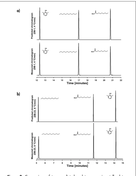
(30) The column axis is divided into small mesh elements, and the subsequent discretization may be performed by approximating the solution with a combination of finite quadratic elements [55]. This makes it possible to solve the full transient convection-diffusion equation (i.e. Equation 1) by reducing the partial differential equation to a system of ordinary differential equations. This will provide detailed information on both retention times and peak widths, since the concentration of all analytes are given in all mesh elements for all timesteps. The retention time of an analyte is given by the time at which the concentration of that analyte reaches its maximum value at the end of the column.. Predicted chromatograms As in the study presented in Paper VI, isothermal retention data in 10 °C increments were acquired. However, in this study using the finite element method (software Comsol Multiphysics (Comsol AB, Sweden)) and the three-parameter equation, a test mixture of 2,6-dimethylphenol, dodecane and methyl decanoate was used. Retention data were collected for four columns with different polarities (DB-1, DB5, DB-17 and DB-23 (Agilent Technologies)). Using Equation 7 to determine the retention coefficients at different temperature, the chromatograms obtained using different temperature programs (with 4 °C/min and 8 °C/min temperature gradients) were predicted for all four columns. Two examples are depicted in Figure 2. The differentces in retention times in the printed chromatograms are almost invisible to the naked eye. In the best predicted case, the discrepancy in retention time is less than 1 s, which corresponds to an average relative error of 0.05%. Even in the least well predicted case, the time difference is only around 2 s. Figure 2 also highlights the fact that the retention order changes as the polarity of the stationary phase changes. The ability of the method to accurately predict the changing positions is more pronounced in Figure 3. This figure depicts all predicted chromatograms obtained for all columns and both temperature programs. The arrows indicate how the elution times are altered.. 30.

(31) a). Time [minutes]. b). Time [minutes]. Figure 2. Comparison of two predicted and two experimentally determined chromatograms. The DB-1 column with a 4 °C/min gradient in the temperature program gave the best prediction (a), whereas the DB-23 column with an 8 °C/min gradient gave the least good prediction (b).. 31.

(32) Time [minutes]. Time [minutes]. Figure 3. Predicted chromatograms resulting from separations of a mixture containing 2,6-dimethylphenol, dodecane and methyl decanoate using four different columns (DB-1, DB-5, DB-17, DB-23) and two different temperature gradients (4 °C/min and 8 °C/min).. 32.

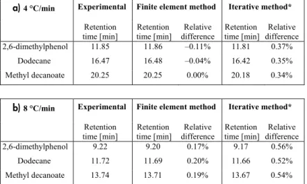
(33) Discretization comparison Illustrative comparisons of some of the retention times obtained with the iterative method, the finite element method and empirical determinations are presented in Table 1. For this evaluation, the same three-parameter model of the temperature dependence of the distribution coefficients was used in the iterative method to the one used in the finite element-based study. For both temperature gradients, the results of the finite element method were substantially better than those obtained with the iterative method. The finite elements method can also provide satisfactory predictions of peak widths. Even though no extra-column effects were considered, the predicted peak widths were only approximately 10% lower than the experimentally determined widths, while there were 40% discrepancies between the results obtained with the iterative method and the experimental data. The main benefit of using the iterative method instead of the finite element method is that it is easier to use, and that the calculations take seconds instead of minutes to perform. Hence, the relative merits of high quality results and rapid computation times must be weighed for specific applications of these measures. Table 1. Comparison between empirically determined and predictions of retention times (for three test substances in a DB-1 column) obtained using Comsol Multiphysics (finite element method) and GC Interactive Simulation (iterative method) software. In both cases three-parameter semiempirical estimations of the retention times were used. (a) Predictions with a 4 °C/min gradient. (b) Predictions with an 8 °C/min gradient. a) 4 °C/min. Experimental. 2,6-dimethylphenol. Retention time [min] 11.85. Retention time [min] 11.86. Relative difference –0.11%. Dodecane. 16.47. 16.48. –0.04%. 16.42. 0.35%. Methyl decanoate. 20.25. 20.25. 0.00%. 20.18. 0.34%. b) 8 °C/min. Experimental. 2,6-dimethylphenol. Retention time [min] 9.22. Retention time [min] 9.20. Relative difference 0.17%. Dodecane. 11.72. 11.69. 0.20%. 11.66. 0.52%. Methyl decanoate. 13.74. 13.71. 0.19%. 13.67. 0.54%. Finite element method. Finite element method. Iterative method* Retention Relative time [min] difference 11.81 0.37%. Iterative method* Retention Relative time [min] difference 9.17 0.56%. *) Unpublished results. 33.

(34) 34.

(35) The enlarged tube method for increased trapping capacity. Breakthrough sampling Before analytes of interest in a sample can be analyzed by gas chromatography, it is often necessary to trap and concentrate them. Several gas enrichment methods based on adsorption are available, such as solid phase micro-extraction [65], and devices such as large size sorptive probes [66]. A common feature of these methods and devices is that they rely on the establishment of partial or complete equilibrium. If the equilibrium values are unknown, subsequent quantification of the analytes may be difficult. However, if the analytes are trapped in an open tubular column trap with a sorptive film, the sample may be driven through the column until a certain amount of analyte exits from the end of the trap. Another advantageous feature of using sorption rather than adsorption is that since the interaction between the analyte and the trapping phase is weaker, high temperatures may not be needed in the subsequent desorption. This is especially advantageous if the analytes are unstable at elevated temperatures [67–69]. The gas volume that has passed the front end of a column before the concentration of the analyte in the effluent gas reaches a determined percentage of the concentration in the inlet gas is often defined as the breakthrough volume VB [70]. The breakthrough volume may be used as a quantitative measure of the trapping capacity, and may be determined from VB = VS ⋅ ( β + K D ) ⋅ f ( L, h, b). (8). where VS is the volume of the stationary sorptive trapping phase and f is a trapping function of the column length (L), the increased disper35.

(36) sion per unit column length (h), and the tolerable level of breakthrough (b). If a breakthrough of 5% is accepted, the trapping function f(L, h, b) in Equation 8 can be written [70] as f ( L, h, b = 0.05) =. 1 5.360h 4.603h 2 0.9025 + + L L2. (9). Open tubular traps are often similar to gas chromatography columns with respect to the materials chosen. However, in contrast to a separation in gas chromatography, the linear velocity of the mobile phase (i.e. of the sample matrix) is not as relevant in practice as the sampling flow rate. To determine the dispersion, it is hence more useful to rewrite Equation 3 in terms of flow rate instead of velocity:. h=. +. 2. πd M2 DM 1 β 2 + 6 K D β + 11K D2 1 F + 2 4 F πDM 24 ( β + K D ). (. 1+ β + β 3( β + KD ). ) 2. 2. KD 1 F πDS. (10). where F is the average volume flow rate of the mobile phase. If the analyte is volatile (and hence has a low distribution coefficient) or very low detection limits are required, the trapping may be difficult since the breakthrough volume must be high to ensure that a sufficient amount of analyte is trapped. As indicated by Equation 8, the breakthrough volume largely depends on the volume of the stationary phase. Thus, one strategy would be to simply increase the length of the tube. However, that approach has the disadvantage that it is limited by the accompanying increase in pressure drop. Another strategy to increase the trapping capacity is to use a large number of short narrow tubes [71, 72]. However, the retention power for highly volatile analytes in such tubes is often unsatisfactory. A more efficient and technically more favorable [71, 73, 74] method is to increase the volume of the stationary phase by making the sorptive film thicker. Provided that the flow rate is sufficiently high to assume negligible static longitudinal diffusion (which applies in most experimental cases), the first term on the right-hand side of Equation 10 equals zero, and the dispersion will hence not depend on the diameter of the column, provided that the phase ratio is kept constant. Consequently, it should be possible to increase the trapping capacity by simultaneously increasing the film thickness and the column diameter. 36.

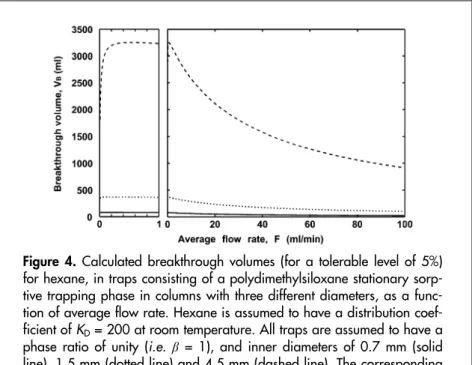
(37) In Figure 4, the calculated breakthrough volumes for hexane in three open tubular traps are depicted [Paper I]. The traps all have the same phase ratio, but different inner diameters (and, hence, different amounts of stationary phase). From this figure, it can be seen that the trap with the largest inner diameter also has the highest breakthrough volume. Even if the flow rate is very large, a high breakthrough volume is achieved. The figure also shows that the trapping volume is only significantly reduced by longitudinal diffusion for the trap with the largest inner diameter.. Figure 4. Calculated breakthrough volumes (for a tolerable level of 5%) for hexane, in traps consisting of a polydimethylsiloxane stationary sorptive trapping phase in columns with three different diameters, as a function of average flow rate. Hexane is assumed to have a distribution coefficient of KD = 200 at room temperature. All traps are assumed to have a phase ratio of unity (i.e. β = 1), and inner diameters of 0.7 mm (solid line), 1.5 mm (dotted line) and 4.5 mm (dashed line). The corresponding sorbent volumes are 0.385, 1.77 and 15.9 ml, respectively.. 37.

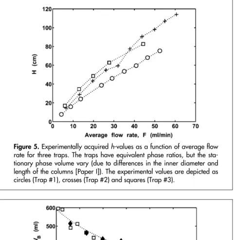
(38) Ultra-thick film enrichment The theoretical conclusions regarding the effects of increased film thickness and diameter were tested experimentally in a series of elution analyses of hexane with three different traps [Paper I], subsequently called Trap #1, Trap #2 and Trap #3 (see Paper 1 for detailed information regarding the traps’ length, phase ratio, etc.). Trap #1 had a phase ratio of circa 1.3, whereas the other two traps (#2 and #3) both had a phase ratio of circa 1.1. In all traps, the gas flow rate through the column was varied, and the dispersion was measured. The dispersions, expressed as H-values, are given in Figure 5. Even though Trap #3 had an inner diameter almost twice as large as that of Trap #2, the dispersions were almost identical at the same flow rates. Trap #1 and Trap #2 had identical inner diameters, but the h-values were lower in Trap #1 due to its higher phase ratio, and probably partly due to its smoother surface. When the values of the trapping function in Equation 8 had been determined, the breakthrough volumes of the three traps were calculated (Figure 6). The predicted and experimental results show good agreement, and for the smooth Trap #1, the differences were tiny. The experimental values for Trap #3 (acquired with both frontal and elution analysis [Paper I]) were less reproducible, but agreed on average with the predicted values. Despite Trap #3 being shorter than Trap #2, its breakthrough volume was more than twice as large. Trap #1 has a lower breakthrough volume since it is only half as long as Trap #3. The experiments confirm that the model for trapping in open tubes with thick films is valid. Thus, it may also be valid to speculate about other implications of the concept. For instance, if a trap with an even larger inner diameter was used, the pressure drop would be low enough to take samples without using pumps. This may be useful for sampling in open air with only the wind as driving force, or for sampling trace volatile analytes in alveolar air using only “lung power”. The limit for the diameter of traps for such applications would probably be set by practical considerations and the fact that a high amount of sorption phase would result in a large desorption volume and high levels of background noise due to sorbent degradation and the sorption of non-target analytes.. 38.

(39) Figure 5. Experimentally acquired h-values as a function of average flow rate for three traps. The traps have equivalent phase ratios, but the stationary phase volume vary (due to differences in the inner diameter and length of the columns [Paper I]). The experimental values are depicted as circles (Trap #1), crosses (Trap #2) and squares (Trap #3).. Figure 6. Predicted and experimental values for the breakthrough volumes (for a tolerable level of 5%) of hexane in the three traps. The predicted values are plotted as curves, whereas the experimental values are depicted as circles (Trap #1), crosses (Trap #2), squares (Trap #3, frontal analysis) and diamonds (Trap #3, elusion analysis).. 39.

(40) 40.

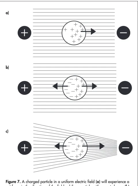
(41) Particle separation with dielectrophoresis. Forces acting on a polarizable particle If a charged particle is placed in an electric field, it will be affected by a force proportional to the electric charge in the direction of the field (Figure 7a). Thus, if the charge is q and the field is E, the force is F =qE. (11). If a particle with no net charge, but with the ability to be polarized is placed in an electric field between two electrodes, the charges in the particle are displaced in the direction towards the electrode with the opposite sign. Thus, the particle will be affected by a force in both directions. Since these two forces are equal in magnitude but have opposite directions, there will be no net movement (Figure 7b). However, if the particle is placed in an electric field that is not uniform, the particle will be affected by a net force in the direction towards the higher field strength (Figure 7c). This phenomenon is called dielectrophoresis [75]. The net dielectrophoretic force FDEP is proportional to the polarizability of the particle and the inhomogeneity of the electric field.. FDEP = (p ⋅ ∇ )E. (12). where p is the induced dipole moment, E is the electric field, and ∇ is the Del operator (gradient). In two Cartesian dimensions, the Del operator is defined as. ⎛ ∂ ∂ ⎞ ∇=⎜ I ⎟ ⎝ ∂ñ ∂ó ⎠. (13). 41.

(42) Particles in chemical applications are often suspended in a liquid medium. If the medium is polarizable and the force on the medium is stronger than the force acting on the particle, the particle will be displaced in the direction towards the lower field strength. This motion is called negative dielectrophoresis. Positive dielectrophoresis will occur when the force on the particle is stronger than the force on the medium, and the particle is moving in the direction towards higher field strength. The induced dipole moment depends on the effective polarizability ~ ( κ ) and the volume (V) of the particle, and the electric field:. ~. p = κ VE. (14). ~ The effective polarizability ( κ ) can be calculated from the shape. of the particle and the dielectric properties (the conductivity and permittivity) of the particle and the surrounding medium. The larger the volume of the particle, the larger the dipole moment will become since the charges may be more separated, whereas the magnitude of the electric field determines how much the charges are displaced. If Equations 12 and 14 are combined, it can be seen that the dielectric force is proportional to the square of the electric field:. FDEP =. κ~V. ∇E. 2. (15). 2 2 2 Since E = − E , the sign of the field has no influence. Thus, if the direction of the field is reversed, the movement will still be in the same direction. Consequently it is possible to use an alternating current (AC) electric field instead of a direct current (DC) electric field. A benefit of this is that the effective polarizability is dependent on the frequency of the applied field. For low frequencies, the effective polarizability will be positive if the conductivity of the particle is larger than the conductivity of the medium, and negative if the conductivity of the medium is larger than the conductivity of the particle. Hence, it is possible to have a movement in the direction towards either higher or lower fields. A positive effective polarizability will result in positive dielectrophoresis, whereas a negative effective polarizability will result in negative dielectrophoresis. For high frequencies, the same rationale can be applied, but with permittivity instead of conductivity.. 42.

(43) a). b). c). Figure 7. A charged particle in a uniform electric field (a) will experience a net force in the direction of the field, while a particle with no net charge (b) experiences no net force. A particle with no net charge but the ability to become polarized will experience a net force towards higher field strength when placed in a non-uniform electric field (c).. 43.

(44) Dielectrophoretic motion In most cases, it is of interest to know the velocity of a particle, rather than to just know the dielectrophoretic force. The velocity induced by dielectrophoretic motion can be written [76] as u abm = ϑabm∇ E. 2. (16). where ϑDEP is the dielectrophoretic mobility. It is impossible to separate particles using dielectrophoresis if not at least one of the parameters affecting the mobility is different between the two sets of species (Note that the parameters influencing the mobility are the permittivity, the conductivity, the size and the shape of the particles, the permittivity, the conductivity and the viscosity of the medium, as well as the frequency of the applied AC electric field). In the subsequent calculations presented in this thesis, the possibilities of exploiting differences in these parameters for separation purposes are explored.. Micro-scale separations of particles using electric forces Separations of micro-particles such as bacteria, yeast cells or polymer beads with different properties are very important in modern material technology and life sciences [77]. The rapid development during the last decade of chip-based micro-systems has had a tremendous impact on these fields [78–81]. Chip-based systems have several advantageous features compared to macroscopic systems, one of which is that the size of biological cells and micro-particles is in the same order of magnitude as the internal dimensions of micro-chip systems. This allows very sensitive methods to be applied, and extremely small samples of just a few (or even single) cells to be manipulated or analyzed. Many different types of forces may be used to manipulate particles in a chip, for instance mechanical, magnetic or optical forces. Electric forces are particularly suitable for miniaturization, because high field strengths can easily be generated with low voltages across small distances. Furthermore, using electric forces, fluid motion can be induced by electro-osmosis, while charged particles can be transported by electrophoresis, and polarizable particles can be manipulated with dielectrophoresis. Electric forces also provide the possibility to study both surface modifications and bulk properties [82–83]. This is useful when studying phenomena such as the effects of drugs on cells, effects of external stimuli on cell behavior or diagnostic aspects of cancers [84]. 44.

(45) Two commonly used methods for separating particles are flow cytometry and field flow fractionation. Bench-top flow cytometers are fast and powerful, but expensive. Normally, flow-cytometric separation requires labeling with, for instance, fluorescent or magnetic markers [85]. This may affect some of the critical properties of the particles such as their viability and function, and it is difficult to downsize the equipment without impairing its performance. A chip-based, label-free technique has been introduced recently, in which the dielectric properties of the particles, measured by impedance spectroscopy, serve as size and or/property indicators prior to flow cytometry [86]. However, the resolution of the system, in terms of size differences, is moderate. Field flow fractionation does not require labeling [87]. The principle of this separation technique is based on differences in hydrodynamic behavior, resulting in differences in the positions of different sets of particles in a laminar fluid stream. Usually, a perpendicular force in the form of a gravitational, thermal, electric or dielectrophoretic field [88, 89] is applied to improve the separation. However, the separation power obtained in practice is modest and there is a great need for improved resolution. As previously mentioned, dielectrophoresis is well suited for manipulating particles in chip-based systems. Dielectrophoresis may be defined as “the motion of polarizable particles in spatially non-uniform electric fields” and was first described by Pohl in the early 1950s [75]. Strong non-uniformity in electric fields was initially difficult to obtain, but improvements in micro-fabrication allowing the production of devices incorporating both micro-electrodes and microchannels has led to widespread use of the method. The dielectrophoretic force is strongest close to the electrode edges, and acts on particles that are either permanent dipoles or polarizable. The direction of the force depends on the polarizability of the particles and the surrounding medium. Usually, dielectrophoretic separation devices are employed as trapand-release-filters or particle sorters. Several methods for trapping and sorting particles dielectrophoretically have been described in the literature [82, 83, 90–95], either to direct one kind of particle to different positions, or to separate particle populations with significant differences in size and/or polarizability. Many types of particles can be separated, for instance different micro-organisms or beads with different surface modifications. Separation by means of dielectrophoresis does not necessarily rely on differences in size or surface proper45.

(46) ties. The bulk properties of the particle may also be important, for instance in separations of viable and non-viable cells [96, 97], where the cells may be of similar size and outer appearance.. 46.

(47) The superpositioned dielectrophoresis concept for improved trapping. Trapping in high conductivity media Fractionating cells is a key step in many biotechnological applications. Furthermore, although maintaining viability is unimportant in some situations, in cases where living micro-organisms are required, e.g. for starter cultures, ensuring the survival of the cells is crucial. One pre-requisite for maintaining viability is to avoid the cells being exposed to excessive osmotic stress by keeping the conductivity of the suspension medium in the same range as the conductivity of the cells. However, this can cause problems for dielectrophoertic separations since their effective polarizability is then low and trapping difficult. Their effective polarizability will, as previously mentioned, affect their mobility. As can be seen from the diagram in Figure 11a, the positive mobility of particles decreases rapidly when the conductivity of the medium is increased, and will eventually decline to zero. In combination with the fact that the dielectric force only affects particles at a small distance from the electrodes, this means that trapping in high conductivity media is not feasible. However, under such conditions, the maximum negative mobility (at a different AC frequency from that used for positive dielectrophoresis) is still high.. Superpositioning of electric fields In the new concept, two AC electric fields with different frequencies are applied to exert a force on a system of particles suspended in a medium (Figure 8). The fields must be considered as superpositioned [98–100], and if the difference between the AC frequencies is sufficiently large (i.e. several orders of magnitude), one of them will in47.

(48) duce positive dielectrophoresis, while the other induces negative dielectrophoresis [Appendix 1]. If uM is the velocity of the suspension medium, and upDEP and unDEP are the respective velocities induced by the positive and negative dielectrophoresis, the total velocity of the particle can be expressed as. u tot =u M +u pDEP +u nDEP. (17). If the fields are opposing each other in a flow channel, it is thus possible to push the particles from one set of electrodes closer to a set of trapping electrodes [Paper II].. Enhanced trapping To investigate the feasibility of enhancing the trapping efficiency using the suggested superpositioned dielectrophoresis approach, calculations on particle trajectories in a micro-system were performed. The trapping was assumed to take place in a flow conduit with the top and the bottom area patterned with micro-electrodes arranged as an interdigitated array [101–104]. The particles were assumed to be trapped if the end point of a trajectory was at an electrode edge. The height of the channel used in this model is approximately 50 times larger than the diameter of the model particle E. coli [105, 106]. As shown in Figure 8c, it is possible to increase the trapping efficiency in media with high conductivity by using a row of electrodes at the top of the channel that pushes the particles into a region closer to the attracting electrodes at the bottom of the channel. This is because with higher conductivities the repelling force of negative dielectrophoresis is stronger than the attractive force of positive dielectrophoresis. In low conductivity media, attracting forces are stronger than repelling forces, and thus in such cases using two attracting arrays would be the preferred choice.. 48.

(49) a) A L0. ¨ 0. 0. b) B L 0. pDEP electrodes. 4L0. pDEP electrodes. ¨ 0. c) C. 0. pDEP electrodes. 4L0. nDEP electrodes. L0. ¨ 0. 0. pDEP electrodes. 4L0. Figure 8. Comparison of cases in which one and two sets of electrodes are used in a high conductivity medium. (a) Only attracting electrodes at the bottom of the channel. The particles in the upper half pass the system without being trapped. (b) Attracting electrodes at both the top and bottom of the channel. The trapping efficiency is increased, but due to the weak dielectrophoretic force at high conductivities, the particles in the middle of the channel escape. (c) The top electrodes are given a repelling AC frequency. At high conductivities, the repelling dielectrophoretic force is stronger than the attracting force. This results in the particles being pushed towards the attracting electrodes at the bottom of the channel. All particles are trapped (see also Paper II).. 49.

(50) 50.

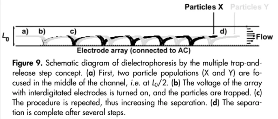
(51) The multi-step dielectrophoresis concept for improved separation. Improving dielectrophoretic separations A common method for separating particles by dielectrophoresis is to use a flow-through system in which one population of particles is trapped while another population of particles is not. Another concept is based on trap-and-release (Figure 9). In the latter method, particles with dissimilar mobilities will travel different distances before they are trapped, and when the voltage is turned off and the particles are released, they will exit the system with some degree of separation. If the difference in mobility between the different populations is sufficiently large, they will be completely fractionated. However, the trapand-release method is not powerful enough if the mobility difference is small. One possibility in such cases is to repeat the trap-and-release procedure several times [Paper III]. As this process is repeated, the degree of fractionation will be gradually enhanced even if two populations are only slightly separated in the first step.. Figure 9. Schematic diagram of dielectrophoresis by the multiple trap-andrelease step concept. (a) First, two particle populations (X and Y) are focused in the middle of the channel, i.e. at L0/2. (b) The voltage of the array with interdigitated electrodes is turned on, and the particles are trapped. (c) The procedure is repeated, thus increasing the separation. (d) The separation is complete after several steps.. 51.

(52) Dielectrophoretic resolution and selectivity To quantify the degree of fractionation obtained with the proposed method using multiple steps, a value for the “dielectrophoretic resolution” (RDEP) is defined as [Paper III]: RDEP =. 3d wA + wB. (18). where d is the distance between the two centers of each particle population, and w is the distance between the particles most far apart within each population. It may either be written as a function of number of separation steps RDEP ( N ) = CR ⋅ N DEP. (19). or as a function of “dielectrophoretic selectivity”, αDEP ,. oabm Eα F = `α ⋅ α abm. (20). where αDEP , is defined as. α abm =. ϑabmIu − ϑabmIv , ϑabmIu > ϑabmIv ϑabmIu. The constants CR and Cα in Equations 19 and 20 are, as well as the dielectrophoretic mobilities (ϑ), describing differences in hydrodynamic and dielectric properties. The term “dielectrophoretic resolution” can also be used to explore the analogy with chromatography. Using the definition in Equation 18, the two particle populations will be completely separated if RDEP > 1.5.. Enhanced separation power As in the example calculated for the superpositioned dielectrophoresis concept, the new method of multi-step dielectrophoresis was demonstrated using a model consisting of a micro-channel with electrode arrays at both the top and bottom of the channel. In this model, dielectric data for polystyrene beads suspended in deionized water were used [107]. At the start of a run, the particles are assumed to be focused in the middle of the channel, and when the voltage is turned on, the particles are transported to different positions downstream in the channel. The distances the particles are displaced before reaching an electrode edge depend on their hydrodynamic and dielectric proper52. (21).

(53) ties. After being trapped, they are released and re-focused in the middle of the channel. If the differences in dielectrophoretic behavior between different sets of particles are sufficiently large, they are completely separated in a single trap-and-release cycle. If the differences are small, the procedure is repeated, leading to increased resolution as the particles move downstream in the channel (Figure 9). Results from the calculation show that it is easier to separate particles with different sizes (Figure 10) than particles with different dielectric properties, since the radius of a particle is quadratically proportional to its mobility, while its dielectric properties are only linearly related to its mobility. In addition, differences in conductivity have a stronger influence on the separation possibilities than differences in permittivity, in accordance with the fact that the conductivity of a particle is mainly governed by its surface properties, whereas its permittivity is determined by bulk properties. A complete separation (i.e. RDEP > 1.5) of particles may be achieved in two trap-and-release cycles if there is a 5% difference in their sizes. If there is a 0.5% size difference, 20 steps are required, and with 200 steps it is possible to separate particles with a size difference as small as 0.2%. For a particle with 5 µm radius, this difference corresponds to a 10 nm coating. As mentioned above, differences in conductivity have a stronger impact on the separation than differences in permittivity. Arnold et al. [107] have shown that the conductivity difference between sets of boiled and unboiled COOH-coated polystyrene beads is 31%. According to the model calculations, this difference is too small to enable complete separation with a single trap-and-release cycle. It should however be possible to separate such particles by repeating the trapand-release cycle only once. Using four steps, the required conductivity difference drops to 19%. Below this level, the separation possibilities are very poor. A reduction in the difference of just a few percent makes separation practically impossible. For situations close to this limit of separation, many cycles would be required. Fifty would correspond to approximately 1500 electrode pairs (assuming that 15 electrodes are utilized in each step). For particles with 5 µm radii, the required channel length would be 15 cm. This is a fairly long channel, but still feasible for a lab-on-a-chip-system [108]. If the differences in dielectric properties are smaller than the critical values required to obtain any separation, some of the values for the system parameters, such as electrode width, electrode gap or voltage must be changed. 53.

(54) a) 2.5. 2. Resolution. Figure 10. Calculated resolution as a function of the number of steps applied in sizebased separation. (a) Relative differences in size: 5%, 2% and 1%. (b) Relative difference in size: 0.5%. (c) Relative difference in size: 0.2%.. 5%. 1.5. 1. 2%. 0.5 1% 0 0. 1. 2 Number of steps. 3. 4. b) 2.5. 2. Resolution. 0.5 % 1.5. 1. 0.5. 0 15. 20 Number of steps. 25. c) 2.5. 2. Resolution. 0.2 % 1.5. 1. 0.5. 0 180. 54. 200 Number of steps. 220.

No results found