ScienceDirect
Available online at www.sciencedirect.com
Procedia Computer Science 130 (2018) 518–525
1877-0509 © 2018 The Authors. Published by Elsevier B.V. Peer-review under responsibility of the Conference Program Chairs. 10.1016/j.procs.2018.04.073
10.1016/j.procs.2018.04.073
© 2018 The Authors. Published by Elsevier B.V.
Peer-review under responsibility of the Conference Program Chairs.
1877-0509 Available online at www.sciencedirect.com
Procedia Computer Science 00 (2018) 000–000
www.elsevier.com/locate/procedia
The 9th International Conference on Ambient Systems, Networks and Technologies
(ANT 2018)
Regression-based evaluation of bicycle flow trend estimates
Johan Holmgren
a,b,∗, Gabriel Moltubakk
a, Jody O’Neill
aaDepartment of Computer Science and Media Technology, Malmö University, Malmö 205 06, Sweden bK2 (The Swedish Knowledge Centre for Public Transport)
Abstract
It has been shown in previous research that regression modeling can be used in order to predict the number of bicycles registered by a bicycle counter. To improve the prediction accuracy, it has also been suggested that a long-term trend curve estimate can be incorporated in a regression problem formulation. A long-term trend curve estimate aims to capture those factors that are difficult, or even impossible, to explicitly model as input variables in the regression model. In the current paper, we present a regression-based approach for evaluating long-term trend curve estimates regarding their possibility to improve the regression prediction accuracy of bicycle counter data. We illustrate our approach by applying it on a time series recorded by a bicycle counter in Malmö, Sweden. For the considered data set, our experimental results indicate that a polynomial of degree two, which has been fitted to the time series, gives the best prediction.
c
�2018 The Authors. Published by Elsevier B.V.
Peer-review under responsibility of the Conference Program Chairs. Keywords: Bicycle counter, regression, trend curve, evaluation
1. Introduction
The bicycle has become an important part of urban transport due to its ability to contribute to fast, sustainable, and cost efficient transport. The bicycle contributes to a healthy, active, life style, and the popularity of the bicycle is accentuated by the increase of bicycling that can be observed around the world. In addition, the bicycle has strong advantages when it comes to parking and storage, as it requires relatively small amount of space. Due to the positive effects of bicycling, there is an increasing interest from public authorities to increase the use of the bicycle. However, in order to achieve a modal shift towards bicycling (from motorized transport), it is important to increase the attractiveness of the bicycle. This can be achieved by implementing various types of policy measures, including the construction and improvement of biking infrastructure, such as bicycling lanes and safe parking facilities. Other
initiatives include bicycle sharing systems, which are currently under development around the world1,2. Bicycle
sharing systems enable, for example, fast multimodal passenger transport, where public transport and the bicycle can
∗Corresponding author. Tel.: +46-40-665 76 88 ; fax: +46-40-665 76 46. E-mail address:johan.holmgren@mau.se
1877-0509 c�2018 The Authors. Published by Elsevier B.V. Peer-review under responsibility of the Conference Program Chairs.
Available online at www.sciencedirect.com
Procedia Computer Science 00 (2018) 000–000
www.elsevier.com/locate/procedia
The 9th International Conference on Ambient Systems, Networks and Technologies
(ANT 2018)
Regression-based evaluation of bicycle flow trend estimates
Johan Holmgren
a,b,∗, Gabriel Moltubakk
a, Jody O’Neill
aaDepartment of Computer Science and Media Technology, Malmö University, Malmö 205 06, Sweden bK2 (The Swedish Knowledge Centre for Public Transport)
Abstract
It has been shown in previous research that regression modeling can be used in order to predict the number of bicycles registered by a bicycle counter. To improve the prediction accuracy, it has also been suggested that a long-term trend curve estimate can be incorporated in a regression problem formulation. A long-term trend curve estimate aims to capture those factors that are difficult, or even impossible, to explicitly model as input variables in the regression model. In the current paper, we present a regression-based approach for evaluating long-term trend curve estimates regarding their possibility to improve the regression prediction accuracy of bicycle counter data. We illustrate our approach by applying it on a time series recorded by a bicycle counter in Malmö, Sweden. For the considered data set, our experimental results indicate that a polynomial of degree two, which has been fitted to the time series, gives the best prediction.
c
�2018 The Authors. Published by Elsevier B.V.
Peer-review under responsibility of the Conference Program Chairs. Keywords: Bicycle counter, regression, trend curve, evaluation
1. Introduction
The bicycle has become an important part of urban transport due to its ability to contribute to fast, sustainable, and cost efficient transport. The bicycle contributes to a healthy, active, life style, and the popularity of the bicycle is accentuated by the increase of bicycling that can be observed around the world. In addition, the bicycle has strong advantages when it comes to parking and storage, as it requires relatively small amount of space. Due to the positive effects of bicycling, there is an increasing interest from public authorities to increase the use of the bicycle. However, in order to achieve a modal shift towards bicycling (from motorized transport), it is important to increase the attractiveness of the bicycle. This can be achieved by implementing various types of policy measures, including the construction and improvement of biking infrastructure, such as bicycling lanes and safe parking facilities. Other
initiatives include bicycle sharing systems, which are currently under development around the world1,2. Bicycle
sharing systems enable, for example, fast multimodal passenger transport, where public transport and the bicycle can
∗Corresponding author. Tel.: +46-40-665 76 88 ; fax: +46-40-665 76 46. E-mail address:johan.holmgren@mau.se
1877-0509 c�2018 The Authors. Published by Elsevier B.V. Peer-review under responsibility of the Conference Program Chairs.
2 Holmgren et al. / Procedia Computer Science 00 (2018) 000–000
be combined in an efficient way1. The fast development of electrical bicycles further increases the attractiveness of the bicycle3.
However, to be able to build a transport system that encourages bicycling, it is important to build knowledge about the current bicycle flows, and what factors are involved in the decision-making of potential bicyclists when choosing whether to use the bicycle, utilize some other mode of transport (e.g., car or bus), or to not travel at all. According to Damant-Sirois and El-Geneidy4, there are four categories of determinants of bicycling: individual characteristics
(including age and gender), individual attitudes (including safety perception and pro-environmental attitude), social environment, and the built environment (i.e., bicycle infrastructure). On the short-term perspective, it has been shown that weather plays an important role whether or not to choose the bicycle5.
Public authorities commonly use bicycle counters, which enable to automatically, and continuously, register the bicycles that pass some strategically chosen points in the traffic network, in order to collect information about the bicycle flows in an urban area. The data produced by a bicycle counter is a time series, where each of the data points in the series corresponds to the number of registered bicycles during a particular time period, for example, an hour or a day. The number of registered bicycles varies over time based on several factors, including the current weather conditions, time of the day, time of the year, and the current interest of the citizens to use the bicycle as a transport mode. In a recent study, Holmgren at al.6
(see also Aspegren & Dahlström7) show how regression can be used in order to quantify how external factors are expected to influence the bicycle traffic flows at a particular point in a traffic network. In particular, they present a regression model that aims to predict the number of bicycles registered by a bicycle counter, using factors such as day of week, season, and weather (temperature and precipitation) as input variables.
In addition to the factors included in the regression model by Holmgren et al.6, there also exist other factors that
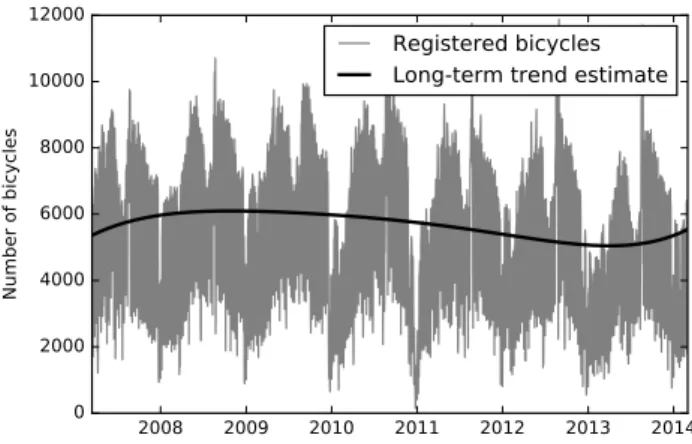
influence how the bicycle flows vary over longer periods time; factors that are difficult to grasp and to explicitly model as input variables in a regression model, for example, since they are not quantifiable using existing data. Examples of such factors are the citizens’ general tendency to use the bicycle and larger infrastructural changes that lead to new patterns of movement. An example of the latter, within the region of our study, is the opening of a new railway station in the center of Malmö in 2010, causing major changes in the traveling pattern for many travelers commuting to and from Malmö. In particular, as the traveling patterns change over longer periods of time, the number of bicycles registered by a bicycle counter is also expected to vary. For example, this implies that the number of bicycles that are registered by the bicycle counter a “normal” day might differ significantly from the number of bicycles registered by the same bicycle counter a normal day a few years later. Using this idea, Holmgren et al.6indicate that there is potential to improve the regression accuracy by incorporating a long term trend estimate taken over the time series produced by a bicycle counter. In order to implicitly capture those factors that are expected to influence the bicycle flow, but which are difficult (or undesirable) to model as input variables, they suggest using the deviation from a long-term trend estimate at the bicycle counter instead of using the absolute number of bicycles as target variable. For illustration, see Fig. 1 for an example of a long term trend curve estimate for a bicycle counter data time series.
There are different ways to construct trend curve estimates for the data points in a time series. For example, trend curve estimates can be generated by fitting polynomial functions of various degrees to the data points in the time series. Another approach is to use splines. However, as trend curve estimates vary in quality and it is possible to construct a very large number of trend curve estimates, it is important to be able to accurately evaluate and compare the quality of different trend curve estimates.
In the current paper, which is based on the Bachelor’s thesis of Moltubakk & O’Neill8, we suggest how to use
regression modeling in order to evaluate trend curve estimates for bicycle counter data time series. We formulate the main tasks included in our evaluation approach as a stepwise procedure, including regression model formulation, generation of trend curve estimates, and evaluation using cross validation on a set of chosen regression algorithms. In addition, we illustrate our approach for regression-based evaluation by applying it on a time series recorded by a bicycle counter in Malmö, Sweden.
Our work aims to provide input for passenger transport analysis models used by city and transport planners, e.g., for assessing the impact of transport policy measures. The relevance in this direction is emphasized by the fact that bicycling is currently being incorporated in passenger transport analysis models around the world. As mentioned above, we present an evaluation method for assessing the quality of long-term trend curve estimates on a time series
Johan Holmgren et al. / Procedia Computer Science 130 (2018) 518–525 519
Procedia Computer Science 00 (2018) 000–000
www.elsevier.com/locate/procedia
The 9th International Conference on Ambient Systems, Networks and Technologies
(ANT 2018)
Regression-based evaluation of bicycle flow trend estimates
Johan Holmgren
a,b,∗, Gabriel Moltubakk
a, Jody O’Neill
aaDepartment of Computer Science and Media Technology, Malmö University, Malmö 205 06, Sweden bK2 (The Swedish Knowledge Centre for Public Transport)
Abstract
It has been shown in previous research that regression modeling can be used in order to predict the number of bicycles registered by a bicycle counter. To improve the prediction accuracy, it has also been suggested that a long-term trend curve estimate can be incorporated in a regression problem formulation. A long-term trend curve estimate aims to capture those factors that are difficult, or even impossible, to explicitly model as input variables in the regression model. In the current paper, we present a regression-based approach for evaluating long-term trend curve estimates regarding their possibility to improve the regression prediction accuracy of bicycle counter data. We illustrate our approach by applying it on a time series recorded by a bicycle counter in Malmö, Sweden. For the considered data set, our experimental results indicate that a polynomial of degree two, which has been fitted to the time series, gives the best prediction.
c
�2018 The Authors. Published by Elsevier B.V.
Peer-review under responsibility of the Conference Program Chairs. Keywords: Bicycle counter, regression, trend curve, evaluation
1. Introduction
The bicycle has become an important part of urban transport due to its ability to contribute to fast, sustainable, and cost efficient transport. The bicycle contributes to a healthy, active, life style, and the popularity of the bicycle is accentuated by the increase of bicycling that can be observed around the world. In addition, the bicycle has strong advantages when it comes to parking and storage, as it requires relatively small amount of space. Due to the positive effects of bicycling, there is an increasing interest from public authorities to increase the use of the bicycle. However, in order to achieve a modal shift towards bicycling (from motorized transport), it is important to increase the attractiveness of the bicycle. This can be achieved by implementing various types of policy measures, including the construction and improvement of biking infrastructure, such as bicycling lanes and safe parking facilities. Other
initiatives include bicycle sharing systems, which are currently under development around the world1,2. Bicycle
sharing systems enable, for example, fast multimodal passenger transport, where public transport and the bicycle can
∗ Corresponding author. Tel.: +46-40-665 76 88 ; fax: +46-40-665 76 46. E-mail address:johan.holmgren@mau.se
1877-0509 c�2018 The Authors. Published by Elsevier B.V. Peer-review under responsibility of the Conference Program Chairs.
Available online at www.sciencedirect.com
Procedia Computer Science 00 (2018) 000–000
www.elsevier.com/locate/procedia
The 9th International Conference on Ambient Systems, Networks and Technologies
(ANT 2018)
Regression-based evaluation of bicycle flow trend estimates
Johan Holmgren
a,b,∗, Gabriel Moltubakk
a, Jody O’Neill
aaDepartment of Computer Science and Media Technology, Malmö University, Malmö 205 06, Sweden bK2 (The Swedish Knowledge Centre for Public Transport)
Abstract
It has been shown in previous research that regression modeling can be used in order to predict the number of bicycles registered by a bicycle counter. To improve the prediction accuracy, it has also been suggested that a long-term trend curve estimate can be incorporated in a regression problem formulation. A long-term trend curve estimate aims to capture those factors that are difficult, or even impossible, to explicitly model as input variables in the regression model. In the current paper, we present a regression-based approach for evaluating long-term trend curve estimates regarding their possibility to improve the regression prediction accuracy of bicycle counter data. We illustrate our approach by applying it on a time series recorded by a bicycle counter in Malmö, Sweden. For the considered data set, our experimental results indicate that a polynomial of degree two, which has been fitted to the time series, gives the best prediction.
c
�2018 The Authors. Published by Elsevier B.V.
Peer-review under responsibility of the Conference Program Chairs. Keywords: Bicycle counter, regression, trend curve, evaluation
1. Introduction
The bicycle has become an important part of urban transport due to its ability to contribute to fast, sustainable, and cost efficient transport. The bicycle contributes to a healthy, active, life style, and the popularity of the bicycle is accentuated by the increase of bicycling that can be observed around the world. In addition, the bicycle has strong advantages when it comes to parking and storage, as it requires relatively small amount of space. Due to the positive effects of bicycling, there is an increasing interest from public authorities to increase the use of the bicycle. However, in order to achieve a modal shift towards bicycling (from motorized transport), it is important to increase the attractiveness of the bicycle. This can be achieved by implementing various types of policy measures, including the construction and improvement of biking infrastructure, such as bicycling lanes and safe parking facilities. Other
initiatives include bicycle sharing systems, which are currently under development around the world1,2. Bicycle
sharing systems enable, for example, fast multimodal passenger transport, where public transport and the bicycle can
∗ Corresponding author. Tel.: +46-40-665 76 88 ; fax: +46-40-665 76 46. E-mail address:johan.holmgren@mau.se
1877-0509 c�2018 The Authors. Published by Elsevier B.V. Peer-review under responsibility of the Conference Program Chairs.
2 Holmgren et al. / Procedia Computer Science 00 (2018) 000–000
be combined in an efficient way1. The fast development of electrical bicycles further increases the attractiveness of the bicycle3.
However, to be able to build a transport system that encourages bicycling, it is important to build knowledge about the current bicycle flows, and what factors are involved in the decision-making of potential bicyclists when choosing whether to use the bicycle, utilize some other mode of transport (e.g., car or bus), or to not travel at all. According to Damant-Sirois and El-Geneidy4, there are four categories of determinants of bicycling: individual characteristics
(including age and gender), individual attitudes (including safety perception and pro-environmental attitude), social environment, and the built environment (i.e., bicycle infrastructure). On the short-term perspective, it has been shown that weather plays an important role whether or not to choose the bicycle5.
Public authorities commonly use bicycle counters, which enable to automatically, and continuously, register the bicycles that pass some strategically chosen points in the traffic network, in order to collect information about the bicycle flows in an urban area. The data produced by a bicycle counter is a time series, where each of the data points in the series corresponds to the number of registered bicycles during a particular time period, for example, an hour or a day. The number of registered bicycles varies over time based on several factors, including the current weather conditions, time of the day, time of the year, and the current interest of the citizens to use the bicycle as a transport mode. In a recent study, Holmgren at al.6
(see also Aspegren & Dahlström7) show how regression can be used in order to quantify how external factors are expected to influence the bicycle traffic flows at a particular point in a traffic network. In particular, they present a regression model that aims to predict the number of bicycles registered by a bicycle counter, using factors such as day of week, season, and weather (temperature and precipitation) as input variables.
In addition to the factors included in the regression model by Holmgren et al.6, there also exist other factors that
influence how the bicycle flows vary over longer periods time; factors that are difficult to grasp and to explicitly model as input variables in a regression model, for example, since they are not quantifiable using existing data. Examples of such factors are the citizens’ general tendency to use the bicycle and larger infrastructural changes that lead to new patterns of movement. An example of the latter, within the region of our study, is the opening of a new railway station in the center of Malmö in 2010, causing major changes in the traveling pattern for many travelers commuting to and from Malmö. In particular, as the traveling patterns change over longer periods of time, the number of bicycles registered by a bicycle counter is also expected to vary. For example, this implies that the number of bicycles that are registered by the bicycle counter a “normal” day might differ significantly from the number of bicycles registered by the same bicycle counter a normal day a few years later. Using this idea, Holmgren et al.6 indicate that there is potential to improve the regression accuracy by incorporating a long term trend estimate taken over the time series produced by a bicycle counter. In order to implicitly capture those factors that are expected to influence the bicycle flow, but which are difficult (or undesirable) to model as input variables, they suggest using the deviation from a long-term trend estimate at the bicycle counter instead of using the absolute number of bicycles as target variable. For illustration, see Fig. 1 for an example of a long term trend curve estimate for a bicycle counter data time series.
There are different ways to construct trend curve estimates for the data points in a time series. For example, trend curve estimates can be generated by fitting polynomial functions of various degrees to the data points in the time series. Another approach is to use splines. However, as trend curve estimates vary in quality and it is possible to construct a very large number of trend curve estimates, it is important to be able to accurately evaluate and compare the quality of different trend curve estimates.
In the current paper, which is based on the Bachelor’s thesis of Moltubakk & O’Neill8, we suggest how to use
regression modeling in order to evaluate trend curve estimates for bicycle counter data time series. We formulate the main tasks included in our evaluation approach as a stepwise procedure, including regression model formulation, generation of trend curve estimates, and evaluation using cross validation on a set of chosen regression algorithms. In addition, we illustrate our approach for regression-based evaluation by applying it on a time series recorded by a bicycle counter in Malmö, Sweden.
Our work aims to provide input for passenger transport analysis models used by city and transport planners, e.g., for assessing the impact of transport policy measures. The relevance in this direction is emphasized by the fact that bicycling is currently being incorporated in passenger transport analysis models around the world. As mentioned above, we present an evaluation method for assessing the quality of long-term trend curve estimates on a time series
520 Holmgren et al. / Procedia Computer Science 00 (2018) 000–000Johan Holmgren et al. / Procedia Computer Science 130 (2018) 518–525 3
Fig. 1. Example of a long-term trend estimate for a bicycle counter data time series.
generated by a bicycle counter. This could be used to improve the modeling of bicycle traffic, and in turn increase the knowledge about how travelers choose their mode of transport.
The current paper is organized in the following way. In the next section we give an account to previous research related to our work. In Section 3 we present our approach for evaluating the quality of trend curve estimates, followed in Section 4 by an experimental illustration of our approach. Finally, we conclude the paper in Section 5.
2. Related work
Due to the increasing interest in the use of the bicycle as a sustainable alternative to motorized transport, the research related to bicycling, in particular bicycle data analysis, has been quite intensive during the recent years. For
example, Romanillos et al.9 provide an overview of big data approaches applied in the bicycling context. A large
amount of research concern bicycle sharing systems, where the studied problems include bicycle repositioning10and location of base (or docking) stations11. Data mining has been applied in the bicycle sharing context, for example, in
order to estimate usage patterns12,13. Data mining also plays an important role in travel demand estimation (including
bicycle demand analysis), which is an integral part of traffic and transport analysis models (both in urban and in regional contexts). Traditionally, travel demand is estimated using travel survey data, often combined with GPS trajectories14. Bicycle demand can be further estimated using different types of discrete choice models, which have
been used, for example, for bicycle route and destination choice estimations15. In addition, there exists research on
how various factors, including weather, calendar events, and work related factors, influence the choice whether or not to use the bicycle16,17. Finally, Holmgren et al.6contribute a regression model, which is able to model how different
factors influence the amount of bicycles that are expected to be registered by a bicycle counter.
3. Regression-based evaluation
In this section, we present our approach for evaluation of bicycle counter data trend curve estimates, which we de-scribe as a stepwise procedure that captures the main tasks involved in the evaluation process. The central component is a regression model, which is formulated in the initial step of the procedure, and which is used in the final step in order to estimate how well different trend curve estimates support the prediction of the data points in a bicycle counter data time series. As mentioned above, a bicycle counter produces a time series consisting of a sequence of data points corresponding to a sequence of non-overlapping, non-separated, equally length, time periods, for example hours or days. For each of the time periods, the corresponding data point specifies the number of registered bicycles during that period. For future reference, we refer to the bicycle counter data time series under consideration as a function f(t) defined over an ordered set of time periods T , where f (t) denotes the number of registered bicycles for period
4 Holmgren et al. / Procedia Computer Science 00 (2018) 000–000
t ∈ T. The generated trend curve estimates are used in the target variable in the regression problem formulation, hence allowing to capture how well different trend curve estimates are able to support the prediction of data points in the time series.
The evaluation procedure consists of the following sequential steps, which will be discussed in more detail below:
Step 1. Formulate regression model.
Step 2. Generate trend curve estimates. Step 3. Select regression algorithms. Step 4. Evaluate trend curve estimates.
It should be emphasized that we did not include any explicit data processing step; instead it is assumed that the data used in the evaluation is processed within the specified steps. However, it should be mentioned that the data processing includes processing of regression model input data (aggregation, normalization, etc.), handling of outliers and missing data values, generation of trend curve estimates and the regression target values used during evaluation, calculation of regression performance values, etc.
3.1. Step 1. Formulate regression model
The purpose of the initial step of the evaluation approach is to formulate the regression problem that will be used later on in order to evaluate the quality of a number of generated trend curve estimates for a bicycle counter data time series. Actually, this step mainly involves selecting which input variables (also called input features), representing factors that potentially influence the amount of bicycle traffic, that should be included in the regression model. It also includes determining the length of the time periods, where each time period corresponds to a data point in the regression problem. It should be mentioned here that it might be desirable to aggregate the data points (i.e., number of registered bicycles) in the time series to form another time series with longer time periods. For example, in the experimental validation presented in Section 4 of the current paper, we used a bicycle counter data time series, where the data points were aggregated from hours to days.
However, it should be noted that selecting an appropriate set of input variables is typically not a trivial task and it normally requires several iterations of refining and evaluating the regression model under development. As we expect that different bicycle counter data time series will be influenced by various factors in different ways, we recommend conducting a variable selection study as part of this step. As a starting point, we suggest using year, day of week, time of year, and weather factors (temperature and precipitation) in the regression model; however, there is a large amount of freedom involved when choosing input variables.
As target variable used in this step, i.e., when selecting an appropriate set of input variables, we suggest using the absolute number of bicycles for each period in the bicycle flow time series. Alternatively, one could use the deviation from the median or from the mean of the time series. Moreover, when experimenting with different sets of input variables, i.e., different regression problem formulations, we suggest testing regression algorithms with different characteristics as different algorithms might perform differently on different data sets.
3.2. Step 2. Generate trend curve estimates
There are many ways to generate trend curve estimates for a time series. Trend curve estimates can be generated, for example, by fitting polynomials of various degrees to the data points in the time series, or by using splines.
As our evaluation approach focus on the evaluation of trend curve estimates, not the generation of estimates, we do not provide any specific guidelines concerning how it is appropriate to estimate trend curve estimates. However, many time series includes seasonal patterns, and we therefore emphasize on the importance to consider this in order to generate trend curve estimates that do not follow the seasonal variations; our idea is that the seasonal variations instead should be captured explicitly by the input variables in the regression model. For later reference we let C denote the set of generated trend curve estimates, each of which can be referred to as a continuous function defined over the considered time period.
Fig. 1. Example of a long-term trend estimate for a bicycle counter data time series.
generated by a bicycle counter. This could be used to improve the modeling of bicycle traffic, and in turn increase the knowledge about how travelers choose their mode of transport.
The current paper is organized in the following way. In the next section we give an account to previous research related to our work. In Section 3 we present our approach for evaluating the quality of trend curve estimates, followed in Section 4 by an experimental illustration of our approach. Finally, we conclude the paper in Section 5.
2. Related work
Due to the increasing interest in the use of the bicycle as a sustainable alternative to motorized transport, the research related to bicycling, in particular bicycle data analysis, has been quite intensive during the recent years. For
example, Romanillos et al.9 provide an overview of big data approaches applied in the bicycling context. A large
amount of research concern bicycle sharing systems, where the studied problems include bicycle repositioning10and location of base (or docking) stations11. Data mining has been applied in the bicycle sharing context, for example, in
order to estimate usage patterns12,13. Data mining also plays an important role in travel demand estimation (including
bicycle demand analysis), which is an integral part of traffic and transport analysis models (both in urban and in regional contexts). Traditionally, travel demand is estimated using travel survey data, often combined with GPS trajectories14. Bicycle demand can be further estimated using different types of discrete choice models, which have
been used, for example, for bicycle route and destination choice estimations15. In addition, there exists research on
how various factors, including weather, calendar events, and work related factors, influence the choice whether or not to use the bicycle16,17. Finally, Holmgren et al.6contribute a regression model, which is able to model how different
factors influence the amount of bicycles that are expected to be registered by a bicycle counter.
3. Regression-based evaluation
In this section, we present our approach for evaluation of bicycle counter data trend curve estimates, which we de-scribe as a stepwise procedure that captures the main tasks involved in the evaluation process. The central component is a regression model, which is formulated in the initial step of the procedure, and which is used in the final step in order to estimate how well different trend curve estimates support the prediction of the data points in a bicycle counter data time series. As mentioned above, a bicycle counter produces a time series consisting of a sequence of data points corresponding to a sequence of non-overlapping, non-separated, equally length, time periods, for example hours or days. For each of the time periods, the corresponding data point specifies the number of registered bicycles during that period. For future reference, we refer to the bicycle counter data time series under consideration as a function f(t) defined over an ordered set of time periods T , where f (t) denotes the number of registered bicycles for period
t ∈ T. The generated trend curve estimates are used in the target variable in the regression problem formulation, hence allowing to capture how well different trend curve estimates are able to support the prediction of data points in the time series.
The evaluation procedure consists of the following sequential steps, which will be discussed in more detail below:
Step 1. Formulate regression model.
Step 2. Generate trend curve estimates. Step 3. Select regression algorithms. Step 4. Evaluate trend curve estimates.
It should be emphasized that we did not include any explicit data processing step; instead it is assumed that the data used in the evaluation is processed within the specified steps. However, it should be mentioned that the data processing includes processing of regression model input data (aggregation, normalization, etc.), handling of outliers and missing data values, generation of trend curve estimates and the regression target values used during evaluation, calculation of regression performance values, etc.
3.1. Step 1. Formulate regression model
The purpose of the initial step of the evaluation approach is to formulate the regression problem that will be used later on in order to evaluate the quality of a number of generated trend curve estimates for a bicycle counter data time series. Actually, this step mainly involves selecting which input variables (also called input features), representing factors that potentially influence the amount of bicycle traffic, that should be included in the regression model. It also includes determining the length of the time periods, where each time period corresponds to a data point in the regression problem. It should be mentioned here that it might be desirable to aggregate the data points (i.e., number of registered bicycles) in the time series to form another time series with longer time periods. For example, in the experimental validation presented in Section 4 of the current paper, we used a bicycle counter data time series, where the data points were aggregated from hours to days.
However, it should be noted that selecting an appropriate set of input variables is typically not a trivial task and it normally requires several iterations of refining and evaluating the regression model under development. As we expect that different bicycle counter data time series will be influenced by various factors in different ways, we recommend conducting a variable selection study as part of this step. As a starting point, we suggest using year, day of week, time of year, and weather factors (temperature and precipitation) in the regression model; however, there is a large amount of freedom involved when choosing input variables.
As target variable used in this step, i.e., when selecting an appropriate set of input variables, we suggest using the absolute number of bicycles for each period in the bicycle flow time series. Alternatively, one could use the deviation from the median or from the mean of the time series. Moreover, when experimenting with different sets of input variables, i.e., different regression problem formulations, we suggest testing regression algorithms with different characteristics as different algorithms might perform differently on different data sets.
3.2. Step 2. Generate trend curve estimates
There are many ways to generate trend curve estimates for a time series. Trend curve estimates can be generated, for example, by fitting polynomials of various degrees to the data points in the time series, or by using splines.
As our evaluation approach focus on the evaluation of trend curve estimates, not the generation of estimates, we do not provide any specific guidelines concerning how it is appropriate to estimate trend curve estimates. However, many time series includes seasonal patterns, and we therefore emphasize on the importance to consider this in order to generate trend curve estimates that do not follow the seasonal variations; our idea is that the seasonal variations instead should be captured explicitly by the input variables in the regression model. For later reference we let C denote the set of generated trend curve estimates, each of which can be referred to as a continuous function defined over the considered time period.
522 Johan Holmgren et al. / Procedia Computer Science 130 (2018) 518–525
Holmgren et al. / Procedia Computer Science 00 (2018) 000–000 5
3.3. Step 3. Select regression algorithms
As different regression algorithms are expected to perform differently on different problems, we recommend using
a set of different regression algorithms when evaluating the generated trend curve estimates. Previous research6
indicate that support vector machines (using 2nd and 3rd degree polynomial kernels) and regression trees work well for the type of problem under consideration. However, it is possible that other regression algorithms will be perform better for a particular data set, which is why we recommend also considering other types of regression approaches.
Altogether, we recommend including a set of different types of regression algorithms (with different characteris-tics), for example, one regression tree, one neural network, support vector regression (using different kernels), and linear regression. A side effect, when comparing the results obtained by different regression algorithms is that one learns about which regression algorithm is expected to perform best on a particular data set.
3.4. Step 4. Evaluate trend curve estimates
The final step of our evaluation approach involves evaluating each of the generated trend curve estimates (c ∈ C) using the regression problem formulation that were defined in Step 1. Using the formulated regression problem, each trend curve estimate should then be evaluated for each of the considered regression algorithms using cross-validation. The regression problem used in this phase makes use of identical input variables and identical input data as the regression problem that were defined in Step 1. The target variable when evaluating a particular trend curve estimate is the relative deviation between the measured number of bicycles and the number of bicycles suggested by the trend curve estimate as target variable.
For trend curve estimate c ∈ C and time period t ∈ T , the deviation devct(i.e., the target variable for curve c and
time period t) is calculated as devct= f(t)−c(t)
c(t) , where f (t) is the number of registered bicycles during time period t and
c(t) is the number of bicycles given by trend curve estimate c during period t. 4. Experimental illustration
In our experimental evaluation, we used a bicycle counter data time series provided by the municipality of Malmö, Sweden. The received time series consist of hourly data from the bicycle counter located at the street Kaptensgatan in Malmö, within the time period September 13, 2006 - March 31, 2014. This bicycle counter is located along one of the main biking routes in Malmö, and in average, it registers approximately 5500 bicycles per day for the time period of the data. As mentioned above, we aggregated the hourly values of the bicycle counter data time series into one data point per day. For the same time period (i.e., September 13, 2006 - March 31, 2014), we downloaded weather data from the open weather data API1provided by the Swedish Meteorological and Hydrological Institute (SMHI). In
particular, we downloaded temperature, precipitation and wind speed. 4.1. Step 1. Formulate regression model
In our experimental validation, we used a regression model formulation that was similar to the regression model formulation used by Holmgren et al.6. Holmgren et al. used year, time of year, day of week, public holiday (yes/no), school break (yes/no), bridge day (yes/no), temperature, and precipitation as input variables.
In the current study, we included wind speed as it might have an influence on the amount of bicycle traffic. We excluded year as the trend curve estimates makes the data points over different years comparable without explicitly modeling year. We also excluded public holiday, school break, and bridge day in order to reduce the number of variables in the problem formulation. In addition, we replaced time of year (a numerical variable taking between 0 and 1) with month (a nominal variable). The input variables used in the current study is presented, together with their value ranges, in Table 1.
In our regression problem formulation, we used time periods of 24 hours; hence we aggregated our original data from hours to days.
1http://opendata-catalog.smhi.se/
6 Holmgren et al. / Procedia Computer Science 00 (2018) 000–000 Table 1. Input variables used in our regression problem formulation.
Input variable (name) Type Value range
is_january, ..., is_december Nominal {0,1}
is_monday, ..., is_sunday Nominal {0,1}
wind speed (daily average) Numerical R
temperature (daily average) Numerical R
precipitation (daily average) Numerical R
4.2. Step 2. Generate trend curve estimates
In our experimental evaluation, we constructed our trend curve estimates using the following steps:
1. First, we generated a yearly moving average time series based on our bicycle counter data, where each data point (a day) is the unweighted mean of the number of bicycles per day for one year centered in that particular day. We calculated the yearly average number of bicycles for a particular day by summing the number of bicycles for all of the days during one year, centered in the current data point, and then dividing with the number of days. 2. We then fitted polynomials of degree 1 to 14, using least squares polynomial fitting, to the yearly moving average
time series, giving us our long-term trend estimates (C).
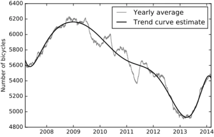
See figure Fig. 2 for an illustration of a trend curve estimate using a polynomial of degree 9. The figure also shows the yearly moving average time series that we used to generate our long-term trend estimates.
Fig. 2. Moving yearly average time series and a nine degree polynomial that was fitted to the yearly moving average time series.
4.3. Step 3. Select regression algorithms
We chose to include the following regression algorithms, all provided by the python module Scikit-learn, in our evaluation of the generated trend curve estimates:
• Support vector machine (SVM), using linear kernel, 3rd degree polynomial kernel, RBF kernel, and sigmoid
kernel.
• Linear Regression
3.3. Step 3. Select regression algorithms
As different regression algorithms are expected to perform differently on different problems, we recommend using
a set of different regression algorithms when evaluating the generated trend curve estimates. Previous research6
indicate that support vector machines (using 2nd and 3rd degree polynomial kernels) and regression trees work well for the type of problem under consideration. However, it is possible that other regression algorithms will be perform better for a particular data set, which is why we recommend also considering other types of regression approaches.
Altogether, we recommend including a set of different types of regression algorithms (with different characteris-tics), for example, one regression tree, one neural network, support vector regression (using different kernels), and linear regression. A side effect, when comparing the results obtained by different regression algorithms is that one learns about which regression algorithm is expected to perform best on a particular data set.
3.4. Step 4. Evaluate trend curve estimates
The final step of our evaluation approach involves evaluating each of the generated trend curve estimates (c ∈ C) using the regression problem formulation that were defined in Step 1. Using the formulated regression problem, each trend curve estimate should then be evaluated for each of the considered regression algorithms using cross-validation. The regression problem used in this phase makes use of identical input variables and identical input data as the regression problem that were defined in Step 1. The target variable when evaluating a particular trend curve estimate is the relative deviation between the measured number of bicycles and the number of bicycles suggested by the trend curve estimate as target variable.
For trend curve estimate c ∈ C and time period t ∈ T , the deviation devct(i.e., the target variable for curve c and
time period t) is calculated as devct= f(t)−c(t)
c(t) , where f (t) is the number of registered bicycles during time period t and
c(t) is the number of bicycles given by trend curve estimate c during period t. 4. Experimental illustration
In our experimental evaluation, we used a bicycle counter data time series provided by the municipality of Malmö, Sweden. The received time series consist of hourly data from the bicycle counter located at the street Kaptensgatan in Malmö, within the time period September 13, 2006 - March 31, 2014. This bicycle counter is located along one of the main biking routes in Malmö, and in average, it registers approximately 5500 bicycles per day for the time period of the data. As mentioned above, we aggregated the hourly values of the bicycle counter data time series into one data point per day. For the same time period (i.e., September 13, 2006 - March 31, 2014), we downloaded weather data from the open weather data API1provided by the Swedish Meteorological and Hydrological Institute (SMHI). In
particular, we downloaded temperature, precipitation and wind speed. 4.1. Step 1. Formulate regression model
In our experimental validation, we used a regression model formulation that was similar to the regression model formulation used by Holmgren et al.6. Holmgren et al. used year, time of year, day of week, public holiday (yes/no), school break (yes/no), bridge day (yes/no), temperature, and precipitation as input variables.
In the current study, we included wind speed as it might have an influence on the amount of bicycle traffic. We excluded year as the trend curve estimates makes the data points over different years comparable without explicitly modeling year. We also excluded public holiday, school break, and bridge day in order to reduce the number of variables in the problem formulation. In addition, we replaced time of year (a numerical variable taking between 0 and 1) with month (a nominal variable). The input variables used in the current study is presented, together with their value ranges, in Table 1.
In our regression problem formulation, we used time periods of 24 hours; hence we aggregated our original data from hours to days.
1 http://opendata-catalog.smhi.se/
Table 1. Input variables used in our regression problem formulation.
Input variable (name) Type Value range
is_january, ..., is_december Nominal {0,1}
is_monday, ..., is_sunday Nominal {0,1}
wind speed (daily average) Numerical R
temperature (daily average) Numerical R
precipitation (daily average) Numerical R
4.2. Step 2. Generate trend curve estimates
In our experimental evaluation, we constructed our trend curve estimates using the following steps:
1. First, we generated a yearly moving average time series based on our bicycle counter data, where each data point (a day) is the unweighted mean of the number of bicycles per day for one year centered in that particular day. We calculated the yearly average number of bicycles for a particular day by summing the number of bicycles for all of the days during one year, centered in the current data point, and then dividing with the number of days. 2. We then fitted polynomials of degree 1 to 14, using least squares polynomial fitting, to the yearly moving average
time series, giving us our long-term trend estimates (C).
See figure Fig. 2 for an illustration of a trend curve estimate using a polynomial of degree 9. The figure also shows the yearly moving average time series that we used to generate our long-term trend estimates.
Fig. 2. Moving yearly average time series and a nine degree polynomial that was fitted to the yearly moving average time series.
4.3. Step 3. Select regression algorithms
We chose to include the following regression algorithms, all provided by the python module Scikit-learn, in our evaluation of the generated trend curve estimates:
• Support vector machine (SVM), using linear kernel, 3rd degree polynomial kernel, RBF kernel, and sigmoid
kernel.
• Linear Regression
524 Johan Holmgren et al. / Procedia Computer Science 130 (2018) 518–525
Holmgren et al. / Procedia Computer Science 00 (2018) 000–000 7
• Lasso
• Bayesian Ridge Regression
We chose this particular set of regression algorithms in order to have different types of linear and non-linear regression approaches represented in our set of algorithms.
4.4. Step 4. Evaluate trend curve estimates
In the final step, we evaluated the generated trend curve estimates using the regression problem that was formulated in Step 1. In this step, we used the relative deviations between the registered number of bicycles and the estimated number of bicycles suggested by the trend curve estimates as target variable. For each of the trend curve estimates, we build regression models for each of the chosen regression algorithms, and evaluated them using the R2correlation
coefficient and 10-fold cross validation. For each of the considered trend curve estimates, we present in Table 2 the R2
correlation coefficient value for the best regression algorithm. For reference, we also present the results when using the median and mean values as trend curve estimates.
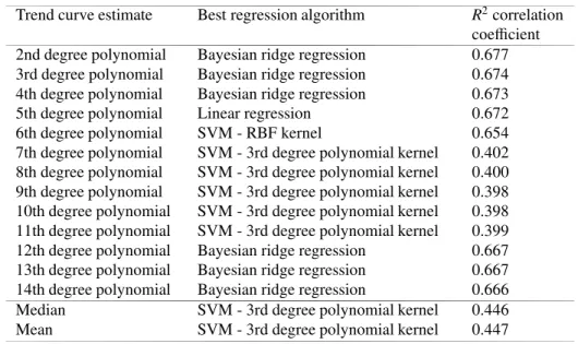
Table 2. For each of the considered trend curve estimates, the R2correlation coefficient value for the best regression algorithm.
Trend curve estimate Best regression algorithm R2correlation
coefficient
2nd degree polynomial Bayesian ridge regression 0.677
3rd degree polynomial Bayesian ridge regression 0.674
4th degree polynomial Bayesian ridge regression 0.673
5th degree polynomial Linear regression 0.672
6th degree polynomial SVM - RBF kernel 0.654
7th degree polynomial SVM - 3rd degree polynomial kernel 0.402
8th degree polynomial SVM - 3rd degree polynomial kernel 0.400
9th degree polynomial SVM - 3rd degree polynomial kernel 0.398
10th degree polynomial SVM - 3rd degree polynomial kernel 0.398
11th degree polynomial SVM - 3rd degree polynomial kernel 0.399
12th degree polynomial Bayesian ridge regression 0.667
13th degree polynomial Bayesian ridge regression 0.667
14th degree polynomial Bayesian ridge regression 0.666
Median SVM - 3rd degree polynomial kernel 0.446
Mean SVM - 3rd degree polynomial kernel 0.447
By using the prediction results where the median and mean of the considered time series were used as trend curve estimate as reference value, our evaluation suggest that our polynomial trend curve estimates of degree 2-6 and 12-14 leads to better predictions (in terms of the R2coefficient value). The polynomial trend curve estimates of degree 7-11 show worse performance than the results of the median and mean trend curve estimates. The best of the analyzed trend curve estimates, according to our results is the 2nd degree polynomial. However, it should be noted that the R2 coefficient values of the eight trend curve estimates that leads to improvements (compared to mean and median) do not differ so much, implying that they are rather similar in performance.
5. Conclusions and future work
We have presented an approach for evaluating long-term trend curve estimates regarding their possibility to improve the regression prediction accuracy of bicycle counter data. The suggested approach is based on regression, and it consists of four sequential steps, which include formulation of the regression problem used for prediction, generation of trend curve estimates, selection of regression algorithms, and evaluation.
8 Holmgren et al. / Procedia Computer Science 00 (2018) 000–000
We illustrated the approach experimentally by applying it on a time series recorded by a bicycle counter in Malmö, Sweden. For the considered data set, our results indicate that a polynomial of degree two, which has been fitted to our bicycle counter data time series (see Section 4.2), gives the best prediction improvement (compared to the case when the median and mean of the time series were used for prediction). One reason why a polynomial of degree two shows best performance according to our evaluation could be that trend curves of higher degree overfits to the data and captures some of the variations that instead should be captured by the variation of the values of the input variables in the regression problem.
It should be emphasized that the approach in its current form gives much freedom, for example, regarding how to formulate the regression problem and which regression algorithms are appropriate to include in the evaluation. It is our belief that some of these choices could be supported in more detail, and future work includes generating guidelines for the different choices included in the approach.
When applying the approach, it is important to be aware of the fact that the variable selection study that typically needs to be conducted in the initial step of the approach is made using a different target variable function than when using the selected features in the final step in order to evaluate the generated trend curve estimates. This issue is something we plan to study in more detail as part of future work.
As future work, we also aim to incorporate the knowledge generated by applying regression modeling on bicycle
counter data in the agent based mode choice model ASIMUT18
, where the decision making of travelers is explicitly modeled. In this respect, it is important to being able to accurately predict the effect on the prediction accuracy of different long-term trend curve estimates, hence enabling to isolate the effects of weather, type of day, etc. when modeling the decision-making of travels. It is our belief that bicycling is one of the key factors to consider when estimating the mode choice of the travelers, as the bicycle is relatively sensitive to the changing weather conditions. References
1. E. Fishman, S. Washington, N. Haworth, Bike share: A synthesis of the literature, Transport Reviews 33 (2) (2013) 148–165.
2. O. O’Brien, J. Cheshire, M. Batty, Mining bicycle sharing data for generating insights into sustainable transport systems, Journal of Transport Geography 34 (2014) 262– 273.
3. T. Jones, L. Harms, E. Heinen, Motives, perceptions and experiences of electric bicycle owners and implications for health, wellbeing and mobility, Journal of Transport Geography 53 (2016) 41–49.
4. G. Damant-Sirois, A. M. El-Geneidy, Who cycles more? Determining cycling frequency through a segmentation approach in Montreal, Canada, Transportation Research Part A 77 (2015) 113–125.
5. M. Nankervis, The effect of weather and climate on bicycle commuting, Transportation Research Part A: Policy and Practice 33 (6) (1999) 417–431.
6. J. Holmgren, A. Sebastian, J. Dahlström, Prediction of bicycle counter data using regression, Procedia Computer Science 113 (2017) 502– 507.
7. S. Aspegren, J. Dahlström, A comparison of machine learning algorithms for estimation of bicycle flows based on bicycle barometer and weather data, Bachelor’s thesis, Malmö University, Sweden (2016).
8. G. Moltubakk, J. O’Neill, Evaluation method of curve fitting for identifying trends in bicycle barometer data, Bachelor’s thesis, Malmö University, Sweden (2018).
9. G. Romanillos, M. Z. Austwick, D. Ettema, J. D. Kruijf, Big data and cycling, Transport Reviews 36 (1) (2016) 114–133.
10. T. Raviv, M. Tzur, I. A. Forma, Static repositioning in a bike-sharing system: models and solution approaches, EURO Journal on Transporta-tion and Logistics 2 (3) (2013) 187–229.
11. J. C. García-Palomares, J. Gutiéerrez, M. Latorre, Optimizing the location of stations in bike-sharing programs: A GIS approach, Applied Geography 35 (1–2) (2012) 235–246.
12. A. K. Datta, Predicting bike-share usage patterns with machine learning, Master’s thesis, University of Oslo, Norway (2014).
13. P. Vogel, T. Greiser, D. C. Mattfeld, Understanding bike-sharing systems using data mining: Exploring activity patterns, Procedia - Social and Behavioral Sciences 20 (2011) 514–523.
14. L. Shen, P. R. Stopher, Review of GPS travel survey and GPS data-processing methods, Transport Reviews 34 (3) (2014) 316–334. 15. J. Hood, E. Sall, B. Charlton, A GPS-based bicycle route choice model for San Francisco, California, Transportation Letters 3 (1) (2011)
63–75.
16. E. Heinen, K. Maat, B. van Wee, The effect of work-related factors on the bicycle commute mode choice in the netherlands, Transportation 40 (1) (2013) 23–43.
17. J. Corcoran, T. Li, D. Rohde, E. Charles-Edwards, D. Mateo-Babiano, Spatio-temporal patterns of a public bicycle sharing program: the effect of weather and calendar events, Journal of Transport Geography 41 (2014) 292–305.
18. B. Hajinasab, P. Davidsson, J. A. Persson, J. Holmgren, Towards an agent-based model of passenger transportation, in: B. Gaudou, J. S. Sichman (Eds.), Multi-Agent Based Simulation XVI: International Workshop, MABS 2015, Istanbul, Turkey, May 5, 2015, Revised Selected Papers, Springer International Publishing, Cham, 2016, pp. 132–145.
• Lasso
• Bayesian Ridge Regression
We chose this particular set of regression algorithms in order to have different types of linear and non-linear regression approaches represented in our set of algorithms.
4.4. Step 4. Evaluate trend curve estimates
In the final step, we evaluated the generated trend curve estimates using the regression problem that was formulated in Step 1. In this step, we used the relative deviations between the registered number of bicycles and the estimated number of bicycles suggested by the trend curve estimates as target variable. For each of the trend curve estimates, we build regression models for each of the chosen regression algorithms, and evaluated them using the R2correlation
coefficient and 10-fold cross validation. For each of the considered trend curve estimates, we present in Table 2 the R2
correlation coefficient value for the best regression algorithm. For reference, we also present the results when using the median and mean values as trend curve estimates.
Table 2. For each of the considered trend curve estimates, the R2correlation coefficient value for the best regression algorithm.
Trend curve estimate Best regression algorithm R2correlation
coefficient
2nd degree polynomial Bayesian ridge regression 0.677
3rd degree polynomial Bayesian ridge regression 0.674
4th degree polynomial Bayesian ridge regression 0.673
5th degree polynomial Linear regression 0.672
6th degree polynomial SVM - RBF kernel 0.654
7th degree polynomial SVM - 3rd degree polynomial kernel 0.402
8th degree polynomial SVM - 3rd degree polynomial kernel 0.400
9th degree polynomial SVM - 3rd degree polynomial kernel 0.398
10th degree polynomial SVM - 3rd degree polynomial kernel 0.398
11th degree polynomial SVM - 3rd degree polynomial kernel 0.399
12th degree polynomial Bayesian ridge regression 0.667
13th degree polynomial Bayesian ridge regression 0.667
14th degree polynomial Bayesian ridge regression 0.666
Median SVM - 3rd degree polynomial kernel 0.446
Mean SVM - 3rd degree polynomial kernel 0.447
By using the prediction results where the median and mean of the considered time series were used as trend curve estimate as reference value, our evaluation suggest that our polynomial trend curve estimates of degree 2-6 and 12-14 leads to better predictions (in terms of the R2coefficient value). The polynomial trend curve estimates of degree 7-11 show worse performance than the results of the median and mean trend curve estimates. The best of the analyzed trend curve estimates, according to our results is the 2nd degree polynomial. However, it should be noted that the R2 coefficient values of the eight trend curve estimates that leads to improvements (compared to mean and median) do not differ so much, implying that they are rather similar in performance.
5. Conclusions and future work
We have presented an approach for evaluating long-term trend curve estimates regarding their possibility to improve the regression prediction accuracy of bicycle counter data. The suggested approach is based on regression, and it consists of four sequential steps, which include formulation of the regression problem used for prediction, generation of trend curve estimates, selection of regression algorithms, and evaluation.
We illustrated the approach experimentally by applying it on a time series recorded by a bicycle counter in Malmö, Sweden. For the considered data set, our results indicate that a polynomial of degree two, which has been fitted to our bicycle counter data time series (see Section 4.2), gives the best prediction improvement (compared to the case when the median and mean of the time series were used for prediction). One reason why a polynomial of degree two shows best performance according to our evaluation could be that trend curves of higher degree overfits to the data and captures some of the variations that instead should be captured by the variation of the values of the input variables in the regression problem.
It should be emphasized that the approach in its current form gives much freedom, for example, regarding how to formulate the regression problem and which regression algorithms are appropriate to include in the evaluation. It is our belief that some of these choices could be supported in more detail, and future work includes generating guidelines for the different choices included in the approach.
When applying the approach, it is important to be aware of the fact that the variable selection study that typically needs to be conducted in the initial step of the approach is made using a different target variable function than when using the selected features in the final step in order to evaluate the generated trend curve estimates. This issue is something we plan to study in more detail as part of future work.
As future work, we also aim to incorporate the knowledge generated by applying regression modeling on bicycle
counter data in the agent based mode choice model ASIMUT18
, where the decision making of travelers is explicitly modeled. In this respect, it is important to being able to accurately predict the effect on the prediction accuracy of different long-term trend curve estimates, hence enabling to isolate the effects of weather, type of day, etc. when modeling the decision-making of travels. It is our belief that bicycling is one of the key factors to consider when estimating the mode choice of the travelers, as the bicycle is relatively sensitive to the changing weather conditions. References
1. E. Fishman, S. Washington, N. Haworth, Bike share: A synthesis of the literature, Transport Reviews 33 (2) (2013) 148–165.
2. O. O’Brien, J. Cheshire, M. Batty, Mining bicycle sharing data for generating insights into sustainable transport systems, Journal of Transport Geography 34 (2014) 262– 273.
3. T. Jones, L. Harms, E. Heinen, Motives, perceptions and experiences of electric bicycle owners and implications for health, wellbeing and mobility, Journal of Transport Geography 53 (2016) 41–49.
4. G. Damant-Sirois, A. M. El-Geneidy, Who cycles more? Determining cycling frequency through a segmentation approach in Montreal, Canada, Transportation Research Part A 77 (2015) 113–125.
5. M. Nankervis, The effect of weather and climate on bicycle commuting, Transportation Research Part A: Policy and Practice 33 (6) (1999) 417–431.
6. J. Holmgren, A. Sebastian, J. Dahlström, Prediction of bicycle counter data using regression, Procedia Computer Science 113 (2017) 502– 507.
7. S. Aspegren, J. Dahlström, A comparison of machine learning algorithms for estimation of bicycle flows based on bicycle barometer and weather data, Bachelor’s thesis, Malmö University, Sweden (2016).
8. G. Moltubakk, J. O’Neill, Evaluation method of curve fitting for identifying trends in bicycle barometer data, Bachelor’s thesis, Malmö University, Sweden (2018).
9. G. Romanillos, M. Z. Austwick, D. Ettema, J. D. Kruijf, Big data and cycling, Transport Reviews 36 (1) (2016) 114–133.
10. T. Raviv, M. Tzur, I. A. Forma, Static repositioning in a bike-sharing system: models and solution approaches, EURO Journal on Transporta-tion and Logistics 2 (3) (2013) 187–229.
11. J. C. García-Palomares, J. Gutiéerrez, M. Latorre, Optimizing the location of stations in bike-sharing programs: A GIS approach, Applied Geography 35 (1–2) (2012) 235–246.
12. A. K. Datta, Predicting bike-share usage patterns with machine learning, Master’s thesis, University of Oslo, Norway (2014).
13. P. Vogel, T. Greiser, D. C. Mattfeld, Understanding bike-sharing systems using data mining: Exploring activity patterns, Procedia - Social and Behavioral Sciences 20 (2011) 514–523.
14. L. Shen, P. R. Stopher, Review of GPS travel survey and GPS data-processing methods, Transport Reviews 34 (3) (2014) 316–334. 15. J. Hood, E. Sall, B. Charlton, A GPS-based bicycle route choice model for San Francisco, California, Transportation Letters 3 (1) (2011)
63–75.
16. E. Heinen, K. Maat, B. van Wee, The effect of work-related factors on the bicycle commute mode choice in the netherlands, Transportation 40 (1) (2013) 23–43.
17. J. Corcoran, T. Li, D. Rohde, E. Charles-Edwards, D. Mateo-Babiano, Spatio-temporal patterns of a public bicycle sharing program: the effect of weather and calendar events, Journal of Transport Geography 41 (2014) 292–305.
18. B. Hajinasab, P. Davidsson, J. A. Persson, J. Holmgren, Towards an agent-based model of passenger transportation, in: B. Gaudou, J. S. Sichman (Eds.), Multi-Agent Based Simulation XVI: International Workshop, MABS 2015, Istanbul, Turkey, May 5, 2015, Revised Selected Papers, Springer International Publishing, Cham, 2016, pp. 132–145.