The real exchange rate: a factor in the economic growth? -The case of Romania-

(1)

The real exchange rate: a factor in the

economic growth?

The case of Romania

Paper within Master thesis in Economics Author: Alexandra-Claudia Minescu

Tutor: Hyunjoo Kim Karlsson

Andreas Stephan

(2)

Abstract

This paper tries to establish if the real exchange rate is a factor in the economic growth. To do so the case of Romania is taken into consideration, a former communist country which at pre-sent has an emergent economy. The bivariate Vector Autoregressive model, Granger causality and the impulse response function have been used in order to see if the real exchange rate has an impact on economic growth which is represented by the Industrial Production Index. The findings suggest that the real exchange rate does not influence the growth of the economy but the other way around, economic growth through the channels of total industry and manufac-turing industry influence in some degree the dynamics of the real exchange rate.

(3)

1. INTRODUCTION ... 1

2. LITERATURE REVIEW ... 2

2.1 Theoretical overview ... 2 2.2 Empirical evidence ... 2

3. DATA ... 5

3.1 The real exchange rate ... 5

3.2 Romania’s external trade ... 6

3.3 Economic growth ... 7

4. METHODOLOGY ... 10

5. EMPIRICAL FINDINGS ... 13

5.1 Unit-root test results ... 13

5.2 Real exchange rate and Total industry ... 14

5.3 Real exchange rate and Mining & Quarrying ... 16

5.4 Real exchange rate and manufacturing ... 17

5.5 Real exchange rate and Electric & Thermal Energy ... 19

5.6 Granger causality tests results ... 20

5.7 Impulse response functions results ... 21

6. CONCLUSIONS ... 23

REFERENCES ... 24

(4)

Figures and tables

Figure 1. Time plots of the real exchange rate of Euro against the Romanian leu

... 6

Figure 2. Romania's Exports ... 7 Figure 3. Romania's Imports ... 7 Figure 4. Industrial production indices for the four industries of Romania 8 Figure 5. Impulse response function- Real exchange rate and Total industry

... 16

Figure 6. Impulse response function- The real exchange rate and Mining & Quarrying industry ... 17 Figure 7. Impulse response function- The real exchange rate and Manufacturing

industry ... 18 Figure 8. Impulse response function- The real exchange rate and Electric and

Thermal Energy industry ... 20 Table 1. Augmented Dickey-Fuller unit-root test results ... 14 Table 2. Granger causality test- Real exchange rate and total industrial index

... 15

Table 3. Granger causality test- Real exchange rate and Mining & Quarrying industry ... 17 Table 4. Granger causality test- Real exchange rate and Manufacturing industry

... 18

Table 5. Granger causality test- Real exchange rate and Electric & Thermal industry ... 19 Table 6. Granger causal relations from the real exchange rate to economic growth proxies ... 21 Table 7. Granger causal relations from the economic growth proxies to the real

(5)

1. INTRODUCTION

The problem of economic growth and the variables that are driving economic growth has been heavily studied throughout the years by numerous researchers. They all agreed on the fact that economic growth can be caused by a variety of factors and also that on its turn it influences other macroeconomic factors such as unemployment, savings or investment.

It is important to establish if there is a connection between some indicators and the economic growth because knowing if such a connection exists there can be measures taken in order to help one country’s economic system to develop and why not to make it be more reliable. This connection is important especially for emerging countries which have a transitioning economy.

Most studies about the Central and Eastern Europe have focused specially on market failure and the process of economic transition because most of these countries had a socialist economy and with the collapse of the socialist regime they had to find ways to overcome the economic crises that followed.

This study tries to establish if there is any connection between the changes experienced by the real exchange rate and the economic growth in a former socialist country that now has an ”emerging country” status.

The country this work focuses its attention upon is Romania. It is chosen because it had a socialist economy before the ’90s and ever since the economy was liberalized it acquired the status of an emerging country. Moreover not many studies investigated the relationship between the real exchange rate and the economic growth in this country. I have used a new approach to the problem by employing the industrial production index. In Romania’s case this index is rather important because the country has a multitude of resources that are not fully exploited and if there is a connection between the real exchange rate and the production outputs maybe more thought will be given to efficiently utilize the resources and thereby increasing the indicators of economic growth.

The rest of the paper is organized as follows. In Section 2 the so far existent literature on the topic is summarized giving the findings and opinions of different researchers in the area. The next sections are closely connected, Section 3 presents the data that will be employed further in the paper, Section 4 defines the steps of the empirical study and Section 5 describes the findings resulted from the analysis. Finally, Section 6 draws the conclusions of the whole paper.

(6)

2. LITERATURE REVIEW

2.1 Theoretical overview

Throughout time there have been many theories of economic growth such as the classical growth theory of Adam Smith or the neoclassical growth model of Solow-Swan that took into consideration equations that showed the relationship between capital goods, output, investment and labor time.

A link between the economic growth and the exchange rate has been investigated more recently and as Eichengreen (2008) emphasizes, ”the real exchange rate has not been at the center of analysis of economic growth. It featured not at all in the first generation of neoclassical growth models or in their practical policy incarnations.”.

There is evidence that one of the conditions for a country’s sustainable economic growth is the continuous growth of labor productivity and economic competitiveness. It is obvious that the most important indicator that quantifies the latter is the equilibrium real exchange rate, a fundamental macroeconomic variable that can be directly observed. This component is very important because the real exchange rate is crucial for the economy due to the fact that it directly influences the external competitiveness of a country especially through export prices. As it was mentioned above, it is known that the real exchange rate works through different channels to influence in some degree the economic growth. The most prominent channel that is discussed in the literature is the one of trade openness. According to some economists such as Balassa (1978) and Edwards (1998) a country should make sure its prices of exportable are high enough to make it attractive to transform the resources into production. This theory is denoted as export-led growth and lead to a growth of production for the export, the real exchange rate being the one providing a motive to shift resources into manufacturing. Hence, the real exchange rate had an impact on economic growth.

As Eichengreen (2008) states, some Asian countries had successfully implemented the export-led growth model thus ”directing the attention to the real exchange rate as a development-relevant policy tool”. This change of attention was not experienced only in Asian countries, but also in most of Latin America and the Caribbean. The overall conclusion of Eichengreen’s study is that ”a stable and competitive real exchange rate should be thought of a facilitating condition for economic growth”.

2.2 Empirical evidence

Even though there are several studies that research the topic of the relationship between the exchange rate and economic growth their results vary because different types of data and methodology are used. For example, some papers analyze the nominal exchange rate while others focus on the real exchange rate. Also the time frame and the country or countries analyzed in the studies are different. In spite of these remarks the main reasoning for studying such relationship is that the changes in the exchange rate lead to uncertainty, which might influence a range of economic variables such as trade, investments and economic growth. The literature on this topic is considering either the volatility of the real exchange rate or the real exchange rate at its level. The former researches are trying to assess that volatility

(7)

dis-as reported by Schnabl (2009) the exchange rate stability in emerging market economies can affect growth if transaction costs for international trade decline and macroeconomic stability is enhanced.

According to Ahmed (2009) ”the volatility of the exchange rate has a negative and major effect both in short run and long run” on the export growth of Bangladesh when North America and Western European countries are examined, but there has been observed no evidence of a connection between the two variables when the exports between Bangladesh and Iran were considered. Of course, an increase in exports induces an increase in the gross domestic product of a country. On the other hand, there are studies that could not establish any kind of link between the exchange rate and international trade (Hooper and Kohlhagen, 1978).

Also, Aghion et all (2009) findings suggest that higher levels of excess exchange rate volatility can have a significant impact on productivity growth and that the financial development is a very important factor for the relationship between the exchange rate regime and long-run growth. They determined that the exchange rate volatility has a significant negative impact on productivity growth and that the more financially developed an economy is the less likely it is affected by this volatility.

Another view on the topic of real exchange rate and economic growth is given by Schanbl (2009) and Bagella et all (2006) as they argue that emerging markets with fixed exchange rates grow faster because this kind of exchange rate has a positive impact on international trade, interest rates and macroeconomic stability. Moreover, it has been examined that in the case of a pegged rate the investments will record an increase, but the economic growth will be lower than in the case of a fixed exchange rate. Despite of this, Ghosh et all (1996) highlights that ” where growth has been sluggish and real exchange rate misalignments common, a more flexible regime might be called for”.

When considering the literature that accounts for the level of the real exchange rate, Dornbusch (1982) affirms that maintaining the real exchange rate at its appropriate level is crucial for economic growth in developing countries, as one of the most important determinants of economic growth is the real exchange rate.

Using panel data estimation from the Central- Eastern European countries, De Grauwe and Schnabl (2004) empirically found a highly significant impact of the exchange rate on real growth. They have established that ”by fixing exchange rates to the euro these countries can reap the benefits of more trade”.

In the recent literature, Rodrik (2007) provides evidence that especially for developing countries where the national currency is depreciated- hence the real exchange rate has a high level- economic growth is stimulated. As he argues,” overvaluation of the currency is one of the most robust imperatives that can be gleaned from the diverse experience with economic growth around the world”. Furthermore, the study states that while an overvaluation has a negative effect on growth1, undervaluation facilitates the economic growth, but this can only happen in developing countries. When the hypothesis was tested for more advanced

1_{The negative effect on growth can be caused by shortage of foreign currency, corruption, large deficits of the}

(8)

economies, the relationship disappeared. It is also considered that real exchange rate is the relative price of tradable to non-tradable goods existent in an economy. The main conclusion drawn from this study is that ”sustained depreciations of the real exchange rate have a positive effect on the profitability of investing in tradable by lightening the economic cost of such distortions, fact that leads to a higher economic growth”. Moreover, Ghura and Grennes (1993) also find that the overvaluation of a currency has an effect on economic growth, this effect suggesting that there is a negative correlation between currency overvaluation and the economic performances of the examined countries.

Eichengreen (2008) studies not just the role of the exchange rate in the growth process, but also the channels through which it influences other variables and the policies used for governing the real exchange rate. He affirms that an increase in the national income is recorded when the real exchange rate is used in order to provide an incentive to shift resources into manufacturing. The incentive is more motivating when the prices of the exportable goods are sufficiently high. One particularly interesting finding is that even though some low- developed countries are successfully using a competitive exchange rate to jump-start growth they need to be aware of the fact that this growth is only for short-term if it is not supported by other fiscal and monetary policies. This theory is supported by evidence from Romania. The gains reported from the nominal depreciation of the national currency were just temporary and on the long run measures that implied productivity growth and correlation of wages with earnings from the increased productivity had to be taken in order to support the economic growth.

As mentioned above, macroeconomic management through policies is very important for growth. If such policies are wrongfully applied, according to Bleaney (1996) they can create uncertainty about relative prices and the absolute price level which discourages investment. He states that poor macroeconomic policy, specially the fiscal balance and the real exchange rate volatility, appears to be associated with low growth for a given rate of investment.

A working paper that overviews the real exchange rate and economic growth in the case of Romania emphasizes the fact that growth can be obtained by more foreign investments which will create more jobs, reduce the rate of unemployment and therefore increase the welfare of the economy. Additionally, the author argues that a depreciation of the national currency is needed so as the exports are increasing, imports are decreasing and the economy will be positively advantaged.

(9)

3. DATA

The empirical part of this paper will focus its attention on an upper middle income European country: Romania. The analysis is based on a time-series data sample of 86 monthly observations covering the period January 2005- February 2012. The data set consists of information for the real exchange rate and the proxy used for the economic growth is the industrial production index. Hence, there will be four variables for the economic growth: Total industry, Mining & Quarrying, Manufacturing and Electric & Thermal Energy.

3.1 The real exchange rate

The real exchange rate is the adjusted nominal exchange rate when taking into consideration the prices on the two markets involved according to the Purchasing Power Parity theory (G. Cassel 1918). In the current paper I will study the Romanian leu (RON) and Euro pair. To compute the real exchange rate I used the Harmonized Consumer Price Index for the Euro area (17 countries) and the same index for Romania. The data was obtained from Eurostat database. Also to calculate the real exchange rate the nominal exchange rate is needed. This was obtained from The National Bank of Romania database. The formula on which these calculations are based is:

The pair RON/EUR was chosen for the real exchnage rate because of the fact that the majority of Romania’s trades are with countries within the European Union and the main currency used is Euro. Therefore it is only natural to use this pair for the present study. Some more details about the external trade of Romania will be given in the next section.

Before 2005 the National Bank of Romania used to frequently intervene on the exchange market in order to facilitate the exports, but starting with 2005 its interventions became less in the context of the liberalization of the capital movement and aiming to discourage speculative attacks.

The evolution of the real exchange rate of the Romanian leu against the Euro is presented in Figure 1, for the analyzed period (January 2005- February 2012). The graph clearly shows that after a continuous real appreciation during 2005, 2006 and 2007, the trend changed. This change is mainly due to the American financial crisis and the effects it had on the global financial market. Also on the first of January 2007 Romania became a member of the European Union and along with this the capital movements from outside the country started to take off.

For the next period (2007-2009) the Romanian leu shows a clear tendency of real depreciation against the Euro, reaching a peak of 3.6185 in January 2009, but starting with 2010 it started to appreciate again.

(10)

Figure 1. Time plots of the real exchange rate of Euro against the Romanian leu

Source: Eurostat, NBR

3.2 Romania’s external trade

Romania has been a part of the European Union since the 1st of January 2004, but it is not a member of the euro zone yet. However, the government is planning to join the euro zone by 2015.

Because the national currency of Romania is still the Romanian leu (RON) most of the trade is made utilizing a more broadly used currency like the Euro or the US Dollar. In the next two figures, the trade volume of exports and imports of Romania within and outside the European Union are presented. The numbers in the graphs are expressed in millions of euro.

As it can be easily seen, the trades of Romania are mostly made within the European Union. Figure 3 summarizes the volume of exports. It is obvious that most of the goods produced in Romania are sold in the countries members of the European Union. A minimum value can be observed at the end of 2008 which could be due to the American financial crises and the recession that followed. Starting with 2009 the exports began to take off and even though they fluctuate, the trend has always been upwards.

The same can be said about Romania’s imports, there is a general upward trend even though there is a structural break at the end of 2008. This structural break can also be seen in Romania’s exports. Putting this information together with the fact that starting with the end of 2007 the Romanian currency started to appreciate in real terms (see Figure 1) it can be concluded that there is a close relationship between the real exchange rate and the trades. All in all, the RON/EUR pair will be used in the study because most of the trades are made inside the European Union and the used currency is the euro.

2 2.5 3 3.5 4 4.5 5 01 -01 -05 01 -06 -05 01 -11 -05 01 -04 -06 01 -09 -06 01 -02 -07 01 -07 -07 01 -12 -07 01 -05 -08 01 -10 -08 01 -03 -09 01 -08 -09 01 -01 -10 01 -06 -10 01 -11 -10 01 -04 -11 01 -09 -11 01 -02 -12

(11)

Figure 2. Romania's Exports

Source: Eurostat

Figure 3. Romania's Imports

Source: Eurostat

3.3 Economic growth

The industrial production index reflects the development of value added in different branches of industry (despite its name) and it is most commonly used to assess the future development of the Gross Domestic Product (GDP) which is available on a monthly basis and it is divided by main industrial grouping. Also this index is one of the “Principal European economic indicators” which are employed to oversee and guide economic and monetary policies in the European Union. Since the changes in the index reflect in some extent the changes in the GDP and ergo in the economic growth I have decided to use the industrial production index as a proxy for the economic growth.

The Total Industry variable takes into consideration all the other three variables, this one being more of an aggregated one. This means that when we are talking about Total Industry

0 500 1000 1500 2000 2500 3000 3500 01 -01 -05 01 -08 -05 01 -03 -06 01 -10 -06 01 -05 -07 01 -12 -07 01 -07 -08 01 -02 -09 01 -09 -09 01 -04 -10 01 -11 -10 01 -06 -11 01 -01 -12 EU Exports Extra-EU Exports 0 500 1000 1500 2000 2500 3000 3500 4000 4500 01 -01 -05 01 -08 -05 01 -03 -06 01 -10 -06 01 -05 -07 01 -12 -07 01 -07 -08 01 -02 -09 01 -09 -09 01 -04 -10 01 -11 -10 01 -06 -11 01 -01 -12 EU Imports Extra-EU Imports

(12)

we are referring to mining and quarrying, manufacturing, electricity, gas, steam and air conditioning supply. The data is seasonally adjusted and taken in percentage change on the previous period.

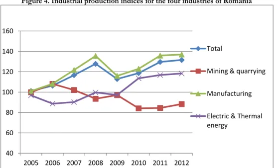
Figure 4 represents the volume index of production for the total industry, mining & quarrying, manufacturing and electric & thermal energy. As it was expected, the predominant industry is the manufacturing industry followed by the electrical & thermal energy and mining & quarrying.

The fact that the mining & quarrying is the industrial sector with the lowest values and a descending trend is somehow surprising because Romania is well-known for its natural resources: large reserves of petroleum, coal, iron ore, salt and others. Also it has the largest oil reserves in Eastern Europe. But these figures make sense when we think that there has been a big lack of investment in this industry which caused the output of everything that relates to mining and quarrying to fall. Likewise, Romania used to be a major oil exporter but now it relies on imports to cover half of its domestic needs. This situation was also produced because of the lack of investment.

The high production volume of the manufacturing industry is due to the foreign investments which started to take of mostly because of the cheap workforce that can be found in Romania. The most attractive industries for the investors are the metallurgic and food industry. Of course there are the clothing and the chemical industries which are considerably large and which have a considerable impact on the total manufacturing industry.

The electric and thermal energy is an important part of the national economy as it provides the electric and thermal energy needed by the other industries and it is an indispensable component of a good development of one’s national economy. A proof to this is the fact that the electric energy production per capita is one of the most important indices when considering one’s country level of development. In the graph below it can be seen that starting with 2007, the production of electric and thermal energy in Romania began to rise. This happened because of the total liberalization of the energy market in 2007.

Figure 4. Industrial production indices for the four industries of Romania

40 60 80 100 120 140 160 2005 2006 2007 2008 2009 2010 2011 2012 Total

Mining & quarrying Manufacturing Electric & Thermal energy

(13)

The data that will be used in the empirical analysis for Mining & Quarrying, Manufacturing and Electric & Thermal Energy is also seasonally adjusted and computed as percentage change of the previous period. As well as the Total Industry variable, the observations were obtained from Eurostat’s database.

(14)

4. METHODOLOGY

As mentioned before, the purpose of this paper is to establish if the real exchange rate influences in any way the economic growth or if economic growth has an impact on the real exchange rate. In order to empirically do this, a series of tests will be used. These tests are described in the following in the order they are employed.

The first step is to examine the time-series property of stationarity. To do this the Augmented Dickey-Fuller (1979) unit-root test will be used with the null hypothesis of non-stationarity (existence of unit-root). In addition to the regular ADF test I will use the Elder & Kennedy strategy (2001) in which a trend component and an intercept will be included. In case one or more of the series is not stationary it will be further tested to check if there is a stochastic or deterministic trend.

In the augmented Dickey-Fuller test it is assumed that the error terms (ut) are correlated and

the main principle of the test is that it is conducted by augmenting the Dickey-Fuller test using p lags of the dependable variable. The model can be written as:

Where β0 is a constant, β1 isthe coefficient on a time trend, p is the lag of order of the

auto-regressive process and ut is a pure white noise error term. The numeric value of p is

deter-mined using Akaike Information Criterion.

When testing for unit roots it is necessary to have a testing strategy. In this paper the Elder & Kennedy strategy (2001) will be employed because it utilizes prior economic theory regarding the tested variables’ expected growth status to establish if a stochastic or deterministic trend can be anticipated. Moreover this strategy rules out some types of unrealistic or implausible outcomes for economic time-series processes such as the co-existence of a unit root and a deterministic trend.

The null hypothesis of this test is that a unit-root exists, meaning that γ=0. The alternative hypothesis is that no unit-root exists in the series which implies γ<0. If the test statistic is less than the critical value then the null hypothesis is rejected, no unit root is present and the time-series is stationary.

In case that all the variables are integrated of the same order a cointegration test should be used in order to check if any cointegrating relationship exists between the variables. Because the variables utilized in this paper have different integration orders, it is not necessary to apply this test.

Since the purpose of this thesis is to analyze aspects of the relationships between the real exchange rate and the economic growth, the bivariate Vector Autoregressive (VAR) model is appropriate to use since it represents the correlations between a set of variables.

The first step in estimating a bivariate VAR model is to determine the optimal lag-length or-der. In order to do so I employed the Akaike Information Criterion.

(15)

The general formula that is going to be used for the bivariate VAR(k) model is as follows: Yt = c + a1 X1t-1 + a2 X1t-2 +…+ ak X1t-k + b1 Yt-1 + b2 Yt-2 +…+ bk Yt-k + ε1t

X1t = c + a1 X1t-1 + a2 X1t-2 +…+ ak X1t-k + b1 Yt-1 + b2 Yt-2 +…+ bk Yt-k + ε2t

where k is the order of the VAR, a is the constant term, ε is an error term, X is a proxy of economic growth and Y denotes the real exchange rate. The model above explains the rela-tionship between the real exchange rate and one of the four proxies for economic growth. After estimating the model we need to make sure the residuals are white noise. If there is white noise, the residuals are completely randomly scattered with no systematic pattern which means that the model is correctly specified and the residuals do not include any information that is not included in the regression. To establish if the residuals are white noise the proper-ties of autocorrelation and normality are tested.

To examine if there is autocorrelation the Breusch-Godfrey serial correlation Lagrange multi-plier test is used. The test will establish if there is any autocorrelation in the errors of the re-gression model. The null hypothesis is that there is no serial correlation of any order up to the specified number of lags and the alternative hypothesis states that there is autocorrelation be-tween the residuals.

In order to see if the residuals are normally distributed the Jarque-Bera normality test is em-ployed. It tests whether the data has skewness and kurtosis matching a normal distribution. The null hypothesis is a joint hypothesis of the skewness being zero and the excess kurtosis being also zero, in other words the null hypothesis states that the data follows a normal distri-bution. Of course, the alternative hypothesis is that the sample data does not follow a normal distribution.

The next step after estimating the models and checking the residuals is to test the direction of the causality using Granger causality test (Granger, 1969). By doing so, the relationship be-tween the variables when they are causing each other can be observed. Having this in mind, one of the four outcomes are possible (Brooks, 2008):

1. If X causes Y, lags of X should be significant in the equation for Y and it can be said that X Granger causes Y;

2. If Y causes X, lags of Y should be significant in the equation for X and it can be said that Y Granger causes X and that there is a unidirectional causality from Y to X;

3. If both variables cause each other it can be said that there is a “bi-directional causality” or “bi-directional feedback”;

4. If neither set of lags are statistically significant in the equation for the other variable it can be said that X and Y are independent.

It is known that it is possible that the Granger causality test by its own may not give a com-plete overview on the interactions that take place among the variables of a system. Because bivariate VAR models will be estimated, it is interesting to observe how a shock in the resid-ual will affect the dependant variables in the VAR model. In order to be able to track this im-pact the impulse response function will be used, in this way producing the time path of the variables in the VAR to shocks from all the explanatory variables. The impulse is given by the Cholesky decomposition.

(16)

Considering the bivariate VAR model above any change in ε1t will immediately change Yt and

in the next period this change in ε1t will also change Xt because Yt-1 is related to Xt in the

second equation. The mentioned change in ε1t will produce a change in Yt as well, since Yt-1 is

related to Yt in the first equation.

(17)

5. EMPIRICAL FINDINGS

Before analyzing the real exchange rate, the real effective exchange rate was employed. The difference between the two is that the real effective exchange rate is the weighted average of a country's currency relative to an index or basket of other major currencies adjusted for the effects of inflation, whereas the real exchange rate is the purchasing power of a currency relative to another.

When using the real effective exchange rate no statistically significant results could be found. The European Central Bank’s real effective exchange rate of 17-Euro area countries vis-a-vis EER-40 group of trading partners was employed. An explanation for this insignificance is that most of the currencies taken against the Romanian leu are not used in the commercial relations of Romania. In other words, currencies like the Canadian dollar or the Polish zlot are not very often traded. Also, another possible explanation is that the more currencies are taken into the index or bascket, the more dispersed the results will be and this will eventually lead to no relationship between the real effective exchange rate and the economic growth.

Moreover, the fact that when using the real exchange rate for the RON/EUR pair, statistically significant results were obtained, suggests that the Euro has a big importance in the Romanian economy.

5.1 Unit-root test results

The results of the Augmented DickeyFuller test suggest that all of the series are stationary -hence they are integrated of order zero I(0)- except for the Real Exchange Rate (RER). This series was further tested to check if there is a stochastic trend, but since the result was not significant the conclusion is that it is a pure random walk. Because of this it was tested again for unit-root and concluded that the series is stationary in the first difference I(1). Table 1 indicates the values of the t-statistic obtained for each time-series both in level and in first difference.

Because the results of the unit-root tests indicate that the series are not integrated of the same order -the proxies used for economic growth are integrated of order zero I(0) and the real effective exchange rate is integrated of order one I(1)- there can be no possibility of cointegrated relationships.

In the bivariate VAR models that are going to be estimated further in this research all the variables will be taken in their first differece. In order to determine the optimal lag length the Akaike Information Criterion will be employed. The VAR lag length order selection criteria are presented in the Appendix.

(18)

Table 1. Augmented Dickey-Fuller unit-root test results

Constrant No constrant Constant and trend Rer 0.257507* 2.924865* -2.251293* Total industry -8.874406 -8.637034 -8.866201 Mining&Quarrying -13.92969 -13.98652 -13.85264 Manufacturing -9.067066 -8.845642 -9.105358 Electric&Thermal energy -7.407223 -7.168452 -7.745835 Rer -6.406015 -5.436077 -6.440193 Total industry -9.328779 -9.387819 -9.352396 Mining&Quarrying -5.285275 -5.31748 -5.242604 Manufacturing -5.794763 -5.842265 -5.788333 Electric&Thermal energy -5.125673 -5.149281 -5.096232 t-Statistic Levels 1 st differences Variable

*denotes that the null hypothesis of unit-root could not be rejected at the 5% and 10% significance level.

The critical values at 5% level of significance for the ADF test with constant is -2.896346, with no constant -1.944713 and with constant and trend -3.464198.

In the following sections four bivariate VAR models will be estimated and for each of them Granger causality test and impulse response functions are employed in order to determine if a causality between the real exchange rate and the proxies of economic growth exists. The bivariate VAR models are as follows:

1. Real exchange rate and Total industry; 2. Real exchange rate and Mining & Quarrying; 3. Real exchange rate and Manufacturing;

4. Real exchange rate and Electric & Thermal Energy.

5.2 Real exchange rate and Total industry

In this part of the paper I will estimate a bivariate VAR model in which the variables are the Real Effective Exchange Rate (RER) and the Total Industry growth (INDT). Based on Akaike’s criterion selection, the optimal lag length is 2. This means that there will be a VAR(2) model.

RERt=0.024770-0.053713RERt-2+0.365950RERt-1 -0.011018INDTt-2 +0.000429INDTt-1+u1t; (0.00735) (0.18020) (0.10754) (0.011018) (0.00365)

[3.39158] [-0.50578] [3.40307] [-3.05133] [0.11729]

INDTt=-0.412214-1.707118RERt-2-0.888870RERt-1-0.0.082540INDTt-2+0.019820INDTt-1+u2t. (0.22595) (0.56547) (0.20684) (0.11171) (0.11307)

[1.82439] [-0.51960] [-0.26718] [-0.73884] [0.17530]

The p-values of each estimate are presented in the round brakets and the t-statistic of the esti-mators are given in the square brackets. A 5% level of significance will be taken into consid-eration.

(19)

As mentioned before, the real exchange rate is a measure of ones country competitiveness, which means that from the model estimated above it can be said that Romania becomes more competitive on the external markets which also implies that the total industry index used as a proxy for the economic growth will increase.

The residuals are normally distributed and not autocorrelated at a 5% significance level, hence they are white noise. Next I will estimate a Granger causality test with the optimal lag length of 2.

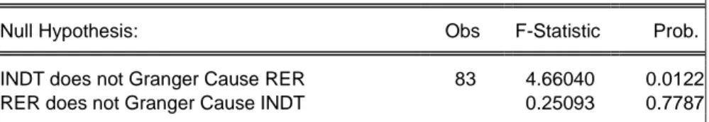
As the table below suggests, at a 5% significance level, the total industrial production Granger causes the real exchange rate. This result is backed up by the bivariate VAR(2) model. As in the VAR the only statistically significant coeficients are the ones for the total industry in the real exchange equation, the result can be interpreted as: if the total industry output will increae by 1%, the real exchange rate will decrease by 0.01% (RON will appreciate) when considering data lagged two. Moreover, if the total industry output will increae by 1%, the real exchange rate will increase very little (real depreciation of the national currency) when considering data lagged one. This implies that whenever there is an increase in the output of the total industry there will be a immediate change in the value of the real exchange rate. The output also implies that there is no bilateral relationship in the sense that the real exchange rate does not cause the total industrial output.

Table 2. Granger causality test- Real exchange rate and total industrial index

Sample: 2005M01 2012M02 Lags: 2

Null Hypothesis: Obs F-Statistic Prob. INDT does not Granger Cause RER 83 4.66040 0.0122 RER does not Granger Cause INDT 0.25093 0.7787

According to the impulse response function a change in the residual will immediately change the real exchange rate. In the next period, this change in the u1t will also change INDTt

(because RERt-1 is related to INDTt in the second equation) and RERt (because RERt-1 is

related to RERt in the first equation). The same thing is true for the next period.

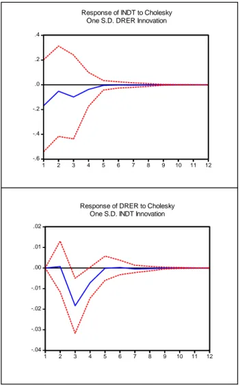
Figure 3 shows the impulse respone function for this pair of variables. The objective of using the impulse response function is to observe the reaction of the system- in this case the system formed of the real exchange rate and the total industry index- to a shock. The dotted lines represent a standard error of +/- 2 in the impulse response function. As it can be seen from the graphs below the responses go to zero, which implies a stable system of equations.

When an impulse is present the real exchange rate’s response to the total industry index is positive for the first two months after which it sharply declines in the third month suggesting a negative effect on the total industry index. Starting with the forth month it is very close to zero indicating that the real exchange rate has no response to the total industry index anymore. When analyzing the response of the total industry index to the real exchange rate it can be observed that it is negative and close to zero for the whole period indicating that if there is a shock the latter variable will experience a fall.

(20)

Figure 5. Impulse response function- Real exchange rate and Total industry

5.3 Real exchange rate and Mining & Quarrying

The variables will be the Real Exchange Rate (RER) and Mining & Quarrying (MQ). The op-timal lag length for this model is one as suggested by the Akiake Information Criterion. The following bivariate VAR(1) model is estimated:

RERt=0.020334+0.345366RERt-1 +0.000701MQt-1+ u1t; (0.00687) (0.10550) (0.06155) [2.96115] [3.36945] [0.45174] MQt=0.158712-10.90979RERt-1 -0.419234MQt-1+u2t. (0.44769) (0.52879) (0.10118) [0.35451] [-0.63226] [-4.14352]

The residuals are normally distributed and not autocorrelated at a 5% significance level, hence they are white noise.

When testing if there is any relationship between these two variables, the output below sug-gests that the real exchange rate does not Granger-causes the mining and quarrying industry or the other way around. Hence, the two variables are independent from each other. This result is in complete agreement with the outcome of the VAR model. As it can be seen, besides the

-.6 -.4 -.2 .0 .2 .4 1 2 3 4 5 6 7 8 9 10 11 12

Response of INDT to Cholesky One S.D. DRER Innovation

-.04 -.03 -.02 -.01 .00 .01 .02 1 2 3 4 5 6 7 8 9 10 11 12

Response of DRER to Cholesky One S.D. INDT Innovation

(21)

constant, none of the estimated coefficients of the bivariate VAR model are statistically insig-nificant, hence there can be no relationship between the variables. To further analyse if one of the variables affects the other I will employ the impulse response function. The results are presented in Figure 4.

Table 3. Granger causality test- Real exchange rate and Mining & Quarrying industry

Sample: 2005M01 2012M02 Lags: 1

Null Hypothesis: Obs F-Statistic Prob. MQ does not Granger Cause RER 84 0.20407 0.6527 RER does not Granger Cause MQ 2.66553 0.1064

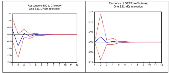
Analysing Figure 4 it can be observed that if there is a one standard deviation shock in the mining and quarrying industry the real exchange rate will have a positive reaction during the first three months after which the shock dies to zero.

When trying to answer the question how is the mining and quarrying industry reacting to the real exchange rate when given a shock, the graph suggests that there will be a fall in the first two months after which the response is very close to zero until the fifth month and after that it is equal to zero. From the graphs it can be concluded that the two variables do not cause each other in the long-run.

Figure 6. Impulse response function- The real exchange rate and Mining & Quarrying industry

5.4 Real exchange rate and manufacturing

In this part of the paper the considered variables are the Real Exchange Rate (RER) and Manufacturing (MAN). According to Akaike’s Information Criterion the optimal lag length is two, hence I will also estimate a bivariate VAR(2) model. The residuals are normally distrib-uted and not autocorrelated at a 5% significance level, hence they are white noise.

RERt=0.025988-0.040050RERt-2+0.338824RERt-1 -0.009249MANt-2 -0.001884MANt-1+ u1t; (0.00728) (0.10580) (0.10747) (0.00304) (0.00307) [3.56906] [-0.37853] [3.15270] [-3.04324] [-0.61257] -2.0 -1.5 -1.0 -0.5 0.0 0.5 1.0 1.5 1 2 3 4 5 6 7 8 9 10 11 12 Response of MQ to Cholesky One S.D. DRER Innovation

-.010 -.005 .000 .005 .010 .015 1 2 3 4 5 6 7 8 9 10 11 12

Response of DRER to Cholesky One S.D. MQ Innovation

(22)

MANt=0.473853-3.130362RERt-2-0.016934RERt-1 -0.039874MANt-2 -0.005387MANt-1+ u2t. (0.26889) (0.98724) (0.76563) (0.11223) (0.11355)

[1.76228] [-0.80121] [-0.00427] [-0.35527] [-0.04745]

If the manufacturing production increases by 1 percent, the real exchange rate will decrease on average by 0.009 percent if it is taken two periods before in time and 0.001 percent if we consider the previous period. These results are to be expected because a high percentage of the manufactured goods are imported and so the real exchange rate appreciates.

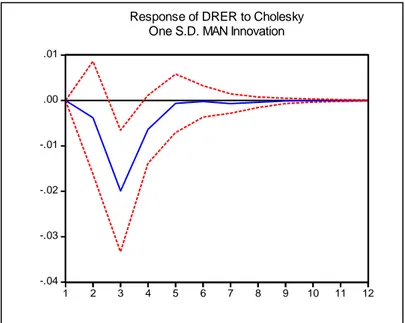
After estimating the VAR(2) model, a Granger causality test based on F-statistic will be esti-mated. The conclusions of this test are that the real effective exchange rate does not Granger cause the manufacturing industry but the manufacturing industry does have an impact on the real exchange rate. The economic meaning of this relationship is that if the manufacturing in-dustry’s output will experience any changes, these changes will be observed in the changes of the real exchange rate.

Table 4. Granger causality test- Real exchange rate and Manufacturing industry

Sample: 2005M01 2012M02 Lags: 2

Null Hypothesis: Obs F-Statistic Prob. MAN does not Granger Cause RER 83 4.78780 0.0109 RER does not Granger Cause MAN 0.36831 0.6931

How will the real exchange rate react to the manufacturing industry if there is a shock? Based on the second graph, the real exchange rate will have a negative response, initially decaying but after a three months period starting to grow. If we want to analyze how the manufacturing industry will react to the real exchange rate in the event of a shock, the answer is given by the first graph which suggests that the response will be negative in the first five months and after this period it reaches zero, indication of the fact that the manufacturing industry has does not cause in any way the real exchange rate after this period.

Figure 7. Impulse response function- The real exchange rate and Manufacturing industry

-.6 -.4 -.2 .0 .2 .4 .6 1 2 3 4 5 6 7 8 9 10 11 12

Response of MAN to Cholesky One S.D. DRER Innovation

(23)

5.5 Real exchange rate and Electric & Thermal Energy

For this bivariate VAR model the variables used are the Real Exchange Rate taken (RER) and Electric & Thermal Energy (ELTH). The optimal lag length suggested by Akaike’s Informa-tion Criterion is 1. The model is:

RERt=0.020245+0.346984RERt-1 -1.05E-05 ELTHt-1+ u1t; (0.00654) (0.10257) (0.08573)

[2.93779] [3.38299] [-0.00608]

ELTHt=-0.595822-4.095908RERt-1 -0.223030ELTHt-+ u2t. (0.46457) (0.98413) (0.12778)

[1.27484] [-0.58880] [-1.89999]

When checking to see if the residuals are white noise, we find that they are normally distrib-uted and that there is no autocorrelation. These results are consistent with white noise.

According to the p-values of the coefficients that were computed by Eviews, none of the coefficients of the real exchange rate or the electric and thermal industry are statistically significant at a 5% significance level.

Regarding if there is any causality between the real exchange rate and the electric and thermal energy industry, the Granger causality test suggests that the two variables are not connected in any way. Either of the variables has no impact on the other. With the help of the impulse re-sponse function I will try to see if the results of this test are further maintained.

Table 5. Granger causality test- Real exchange rate and Electric & Thermal industry

Sample: 2005M01 2012M02 Lags: 1

Null Hypothesis: Obs F-Statistic Prob. ELTH does not Granger Cause RER 84 3.7E-05 0.9952 RER does not Granger Cause ELTH 0.34669 0.5576

-.04 -.03 -.02 -.01 .00 .01 1 2 3 4 5 6 7 8 9 10 11 12

Response of DRER to Cholesky One S.D. MAN Innovation

(24)

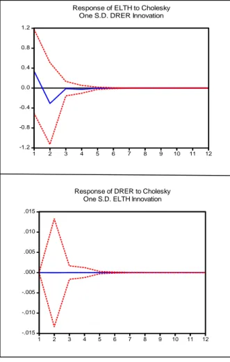
When computing the impulse-response function for this bivariate VAR model, it can be ob-served in Figure 6 that the response of the real exchange rate to the electric and thermal indus-try is zero (unlike the responses of the real exchange rate to the other variables) throughout the entire period.

There can also be noticed differences in the response of the electric and thermal energy to the real exchange rate when a shock is present compared to the responses of the other variables to the real exchange rate. In this case, the response is positive in the first month and continues to grow very little after declining in the second month.

Because both the responses of the real exchange rate and of the electric and thermal energy to the electric and thermal energy and real exchange rate respectively are going to zero in the long-run it is safe to conclude that the two variables are independent from each other- a change in one of them will not entail a response in the other one.

Figure 8. Impulse response function- The real exchange rate and Electric and Thermal Energy industry

5.6 Granger causality tests results

According to the Granger causality tests conducted earlier on in this paper, it can be con-cluded that the real exchange rate has no impact on the four proxies used for the economic growth, but as the results suggest the total industrial and manufacturing output do influence

-1.2 -0.8 -0.4 0.0 0.4 0.8 1.2 1 2 3 4 5 6 7 8 9 10 11 12

Response of ELTH to Cholesky One S.D. DRER Innovation

-.015 -.010 -.005 .000 .005 .010 .015 1 2 3 4 5 6 7 8 9 10 11 12

Response of DRER to Cholesky One S.D. ELTH Innovation

(25)

The p-values obtained when testing if the economic growth Granger-causes the real exchange rate are presented in Table 6. It is obvious that at a 5% significance level only the total indus-try and the manufacturing indusindus-try are the ones that influence the dependant variable. From these two Granger-causalities, the one stating that the manufacturing industry influences the real exchange rate is statistically more significant than the real exchange rate- total industry causality. These results prompt that any change in the outputs of the before mentioned indus-tries will involve a change in the real exchange rate. Also, the results are not very surprising considering that from all the industries, the manufacturing industry is the one with the highest output.

Table 7 provides an overview of the results obtained when testing if the real exchange rate (through the proxies used) Granger-causes economic growth. Even at a 10% significance level the results are statistically insignificant. This suggests that the real exchange rate does not have any influence on the proxies.

Considering the results of the Granger-causality test, when the pairwise combinations between the real exchange rate and the minig & quarrying and electric & thermal energy industries are investigated, it can be concluded that these variables are independent from each other.

Table 6. Granger causal relations from the real exchange rate to economic growth proxies P-value

Total industry 0.0122

Mining & Quarrying 0.6527

Manufacturing 0.0109

Electric & Thermal Energy 0.9952

Table 7. Granger causal relations from the economic growth proxies to the real exchange rate P-value

Total industry 0.7787

Mining & Quarrying 0.1064

Manufacturing 0.6931

Electric & Thermal Energy 0.5576

5.7 Impulse response functions results

The impulse response functions trace the responsiveness of the dependent variable in the VAR model to shocks to each of the variables. In other words, a unit shock is applied to the error for each variable of every equation and the effects on the VAR system over time are noted. If we take a look at the graphs that show the response of the real exchange rate to the total in-dustry and to the manufacturing inin-dustry it can be said that when any of these industries ex-perience an innovation there will be a negative effect on the real exchange rate. This negative effect is more pronounced in the first three months and starting with the fourth month it starts to increase and go to zero. In the case of the response of the real exchange rate to the mining and quarrying industry the situation is slightly different. Any innovation in this industry will have a positive effect on the real exchange rate. As well as in the case of the total industry, in the first two months the response of the real exchange rate is positive but after this it begins to decline to zero. Considering the response of the real exchange rate to the electric and thermal energy industry the results are different from the others. Throughout the whole analyzed

(26)

pe-riod the response is equal to zero suggesting that this industry has no implications on the real exchange rate.

When comparing the responses of the proxies for the economic growth to the real exchange rate it can be concluded that any innovation will eventually lead to a zero response of the proxies implying that the shock will not effect in any way the economic growth.

(27)

6. CONCLUSIONS

The purpose of this paper was to establish if there is any kind of relationship between the real exchange rate and the economic growth of an emerging European country and in which way this relationship -if it exists- works. The country chosen is Romania because it fits the concept of “emerging” country and also from the 27 countries that form the European Union, Romania is situated in the group of upper middle income countries.

Likewise, the subject of the thesis is a very important one for this country because for the last years Romania is fighting to surpass the poor economic system and achieve the status of a de-veloped country.

Recently the study of the real exchange rate as an engine of economic growth has been con-sidered by plenty articles, but most of them concentrated on the Asian markets or Western Europe. The empirical analysis focused on Eastern Europe countries are scarce which is why I chose to contribute to it by taking the case of Romania.

It has been shown that the economic growth partly influences in some degree the real ex-change rate (RON/EUR).

The study suggests that the real exchange rate is influenced by the manufacturing industry as well as the total industry, but no relationship whatsoever was found between the real exchange rate and the electric and thermal energy industry or between the real exchange rate and the mining and quarrying industry. The results indicate that in the case of an increased output in the two mentioned industries the dynamics of the real exchange rate will modify.

(28)

REFERENCES

Aghion, P., (2009), "Exchange rate volatility and productivity growth: the role of financial development." Journal of monetary economics, 56, 494-513;

Ahmed, S. (2009), “An empirical study on exchange rate volatility and its impacts on bilateral export growth: evidence from Bangladesh“, MPRA paper No. 19855;

Balassa, B., (1978), ”Exports and economic growth:further evidence”, Journal of

Development Economics, 5, 181-189;

Bleaney, M.F., (1996), “Macroeconomic stability, investment and growth in developing countries”, Journal of Development Economics, 48, 461-477;

Brooks, C., (2008), “Introductory Econometrics for Finance”, Second edition, Cambridge University press;

Cassel, G., (1918), “Abnormal Deviations in International Exchanges”, The Economic

Journal, 28, 413-415;

Dickey, D.A. and W.A., Fuller, (1979), “Distribution of the Estimators for Autoregressive Time Series with a Unit Root”, Journal of the American Statistical Association, 74, 427–431; Dornbusch, R., (1982), “Equilibrium and Disequilibrium Exchange rate”, M.I.T. Working

Paper, 309;

Edwards, S., (1998), ”Openness, productivity and growth: what do we really know?”, The

Economic Journal, 108, 383–398;

Eichenbaum, M., (1992), Comments “Interpreting the macroeconomic time series facts: the effects of monetary policy” by Christopher Sims, European Economic Review, 36, 1001-1011;

Eichengreen, Barry, (2008), “The real exchange rate and economic growth”, World Bank, Working paper, No. 4;

Elder J. and Kennedy P.E., (2001), “Testing for Unit Roots: What Should Students be Taught?”, Journal of Economic Education, 32, 137-146;

(29)

Ghiba, N., (2010), “Exchange rate and economic growth. The case of Romania.” ,CES

Working Papers, II, 4;

Ghosh, A.R., Gulde, A.-M., Ostry, J.D., Wolf, H., (1996), ”Does the exchnage rate regime matter for inflation and growth?”, Economic issues, Vol. 2, International Monetary Fund, Washington, D.C.;

Ghura, D., Grennes, T.J., (1993), ”The real exchange arte and macroeconomic performance in Sub-Saharan Africa”, Journal of Development economics”, 42, 155-174;

Granger, C.W.J., (1969), "Investigating Causal Relations by Econometric Models and Cross- Spectral Methods”, Econometrica, 37, 24-36;

Grauwe, P. D. and G. Schnabl (2004), “Exchange rate regimes and macroeconomic stability in central and eastern Europe”, CESIFO Working Paper No. 1182;

Gujarati, D.N., (2004), “Basic Econometrics”, Forth edition, The McGraw-Hill Companies; Hooper, P., Kohlhagen, S.W. (1978), “The effect of exchange rate uncertainty on the prices and volume of international trade”, Journal of International Economics, 8, 483-511;

Rodrik, Dani, (2008), “The real exchange rate and economic growth” Brookings Papers on

Economic Activity, Fall, 365-412;

Schnabl, G., (2009), ”Exchange rate volatility and Growth in Emerging Euroope and East Asia”, Open Economies Review, 20, 565-587;

Sims, Christofer A., Stock, James H., Watson, Mark W., (1990), “Inference in Linear Time Series Model with some Unit Roots”, Econometrica, 58, 113-144;

Sims, Christopher A., 1980, “Macroeconomics and Reality,” Econometrica, 48, 1-48;

Swanson, N. and C.W.J., Granger (1997), “Impulse response functions based on the causal approach to residual orthogonalization in vector autoregressions”, Journal of the American

(30)

APPENDIX

Augmented Dickey-Fuller unit-test results

Real exchange rate- level

Null Hypothesis: RER has a unit root Exogenous: Constant, Linear Trend

Lag Length: 1 (Automatic based on AIC, MAXLAG=11)

t-Statistic Prob.* Augmented Dickey-Fuller test statistic -2.251293 0.4553 Test critical values: 1% level -4.071006

5% level -3.464198 10% level -3.158586 *MacKinnon (1996) one-sided p-values.

Real exchange rate- first difference

Null Hypothesis: RER has a unit root Exogenous: Constant, Linear Trend

Total industry index- level

Null Hypothesis: INDT has a unit root Exogenous: Constant, Linear Trend

Mining & Quarrying industry- level

Null Hypothesis: MQ has a unit root Exogenous: Constant, Linear Trend

5% level -3.463547 10% level -3.158207

(31)

Manufacturing industry- level

Null Hypothesis: MAN has a unit root Exogenous: Constant, Linear Trend

Electric and Thermal industry- level

Null Hypothesis: ELTH has a unit root Exogenous: Constant

VAR Lag Order Selection Criteria

Real exchange rate- Total industry index

Sample: 2005M01 2012M02 Included observations: 80

Lag LogL LR FPE AIC SC HQ

0 -41.63763 NA 0.010206 1.090941 1.150491* 1.114816* 1 -36.27519 10.32271 0.009865 1.056880 1.235532 1.128506 2 -31.08526 9.731111* 0.009578* 1.027132* 1.324885 1.146509 3 -30.31405 1.407456 0.010389 1.107851 1.524706 1.274980 4 -29.80745 0.899220 0.011349 1.195186 1.731142 1.410066 5 -26.09680 6.400878 0.011449 1.202420 1.857477 1.465051 * indicates lag order selected by the criterion

(32)

Real exchange rate- Mining & Quarrying industry

0 -117.2137 NA 0.067515 2.980341 3.039892 3.004217 1 -102.4187 28.48035* 0.051549* 2.710467* 2.889119* 2.782093* 2 -99.70756 5.083326 0.053251 2.742689 3.040442 2.862067 3 -98.98730 1.314478 0.057834 2.824683 3.241537 2.991811 4 -95.89693 5.485412 0.059225 2.847423 3.383379 3.062303 5 -92.68838 5.534748 0.060504 2.867209 3.522267 3.129841 * indicates lag order selected by the criterion

Real exchange rate- Manufacturing industry

0 -56.25328 NA 0.014707 1.456332 1.515883* 1.480208* 1 -50.72751 10.63711 0.014158 1.418188 1.596840 1.489814 2 -45.63732 9.544107* 0.013781* 1.390933* 1.688686 1.510311 3 -44.72326 1.668148 0.014894 1.468082 1.884936 1.635211 4 -43.51782 2.139668 0.015988 1.537945 2.073901 1.752826 5 -39.06148 7.687175 0.015832 1.526537 2.181594 1.789168 * indicates lag order selected by the criterion

Real exchange rate- Electric and Thermal industry

0 -112.5640 NA 0.060106 2.864101 2.923651* 2.887976 1 -105.2015 14.17296* 0.055263* 2.780036* 2.958688 2.851663* 2 -102.8420 4.423890 0.057592 2.821051 3.118804 2.940429 3 -100.4231 4.414541 0.059948 2.860578 3.277433 3.027707 4 -98.84841 2.795100 0.063760 2.921210 3.457166 3.136090 5 -93.79736 8.713068 0.062205 2.894934 3.549991 3.157565 * indicates lag order selected by the criterion

The real exchange rate: a factor in the economic growth? -The case of Romania-