Underpricing and underperformance of Swedish IPO’s : A comparative study of different sectors from 2007-2017

(1)

Underpricing and underperformance of

Swedish IPO’s

MASTER THESIS WITHIN: Business administration NUMBER OF CREDITS: 30 ECTS

PROGRAMME OF STUDY: Civilekonomprogrammet TUTOR: Agostino Manduchi & Toni Duras

AUTHOR: Henry Björkqvist & Gustav Kallén JÖNKÖPING May 2018

A comparative study of different sectors

from 2007-2017

(2)

Acknowledgements

We want to extend our gratitude towards our tutors Agostino Manduchi and Toni Duras for your advice and guidance during the writing process. We would also like to thank the members of our seminar group for your helpful remarks.

(3)

Master Thesis within Finance

Title: Underpricing and underperformance of Swedish IPO’s – A comparative study of

different sectors from 2007-2017

Authors: Henry Björkqvist & Gustav Kallén

Tutor: Agostino Manduchi & Toni Duras

Date: 2018-05-21

Key terms: IPO underpricing, IPO underperformance, IPO sectors, Swedish IPO’s

Abstract

Background: The post-IPO anomalous behaviour in the short and long-run are among the

well-recognised anomalies in corporate finance, and exist on all equity markets. The researchers are not unanimous what causes these phenomena’s, and previous research has primarily focused on the US and European markets.

Purpose: The study aims to investigate the market performance of Swedish IPO's in the short- and

long-run in-between 2007-2017 for different sectors.

Method: The market adjusted initial return method was used to calculate the short-run initial return.

The Even-time approach with the Buy-and-hold methodology was used to calculate the long-run abnormal returns. A regression analysis was adopted to investigate the relationship between some existing theories for explaining underpricing.

Conclusion: Overall the sample set for the study were on average underpriced with 9,25 %,

furthermore, no evidence was found that Swedish IPO’s underperformed in a three-year period compared to the market. Of the theories tested, the signalling hypothesis was significant and can be one determinant for underpricing of Swedish IPO’s.

(4)

Acknowledgements ... i

Abstract ... ii

Table of Contents ... iii

1. Introduction ... 1

1.1 Background ... 1

1.1.1 Short-run underpricing ... 2 1.1.2 Long-run underperformance ... 2

1.2 Problem statement ... 3

1.3 Purpose ... 4

1.3.1 Research problem ... 4

1.4 Scope and Limitations ... 4

1.5 Definitions ... 5

2. Frame of References ... 6

2.1 Theoretical Framework ... 6

2.1.1 Theoretical explanations of short-run underpricing ... 7

2.1.2 Theoretical explanations for long-run underperformance ... 9

2.1.3 “Hot issue markets” phenomena ... 10

2.2 Previous studies on short-run underpricing ... 11

2.3 Previous studies on long-run underperformance ... 12

3. Data Method & Methodology ... 14

3.1 Introduction to method ... 14

3.2 Research strategy ... 14

3.3 Research method ... 14

3.4 Methodology on short-run underpricing ... 17

3.4.1 Calculation of the first-day return ... 17

3.4.2 Testing for statistical significance ... 17

3.4.3 Multiple regression model - ordinary least squares (OLS) ... 18

3.5 Methodology on long-run underperformance ... 23

4. Empirical Results... 27

4.1 Results for the short-run market performance ... 27

4.1.1 Descriptive statistics ... 27

4.1.2 Tests for statistical significance ... 30

4.1.3 Multiple regression analysis ... 32

4.2 Results for the long-run market performance ... 36

4.2.1 Descriptive statistics ... 36

5. Analysis ... 38

5.1 Short-run underpricing... 38

5.2 Long-run underperformance ... 41

6. Conclusion ... 42

7. Discussion ... 43

7.1 Future Studies ... 43

7.2 Societal and Ethical Issues ... 44

8. Bibliography ... 45

Appendix 1 ... 49

Appendix 2 ... 54

(5)

Appendix 6 ... 63

Appendix 7 ... 64

List of Figures

Figure 1. Average initial return for selected countries ... 11

Figure 2. Long-run aftermarket performance for selected countries ... 13

Figure 3. IPO activity 2007-2017 ... 28

Figure 4. Distributions of IPO in different sectors ... 29

Figure 5. Average underpricing per sector ... 31

Figure 6. Histogram for dependent variable ... 34

Figure 7. Heteroscedasticity ... 35

Figure 8. Long-run IPO Activity ... 37

List of Tables

Table 1. Overview of existing theories of underpricing ... 7

Table 2. Swedish Studies in long-run underperformance ... 13

Table 3. Assumption in the OLS regression ... 21

Table 4. Descriptive statistics of post day returns ... 27

Table 5. One Sample Student t-test ... 30

Table 6. Descriptive statistics for sectors ... 31

Table 7. Multiple regression output. ... 32

Table 8. Statistics of Independent variables ... 33

Table 9. Jarque-Bera test ... 33

Table 10. Correlation Matrix ... 35

Table 11. 3-year buy and hold abnormal returns for Swedish IPO ... 36

Table 12. Long-run return for different sectors ... 36

(6)

Chapter 1: Introduction

1. Introduction

The following paragraph aims to give the reader a general introduction to an Initial public offering (IPO) and present the two anomalies which characterise IPO’s; short-run underpricing and the long-run underperformance phenomena’s.

1.1 Background

The acronym IPO stands for “initial public offerings” which is the terminology used on the first occasion when the public can purchase stocks from a previously privately owned firm and marks the transition from private to public ownership (Black, Hashimzade & Myles, 2017). Going public allows the firm to access the public capital which may be used to pay off debt, business development, and growth or expansion. IPO’s are an influential component of financial economics since high-growth firms tend to generate new jobs and create revenue (Kulendran & Perera, 2016).

Although the benefits of initial public offerings (IPO) appear to be lucrative for the parties involved, empirical studies have since the 1960’s documented the existence of two post-IPO anomalous behaviours which is among the most well-recognised anomalies in the field of corporate finance (Abrahamsson & De Ridder, 2015). First, new issues generally tend to have a significant increase from the offer price on the first-day trading which offers an exploitable trading opportunity since investors can benefit from the price change. Second, firms going public tend to underperform for 1-5 years compared with more established firms, which questions if it is a favourable investing strategy to hold new issues for a more extended period (Ritter, 1991).

The short-run and long-run anomalies are a universal problem and have received considerable attention in the finance literature since there are significant and persistent variations in the post-IPO returns, contravening the basic idea of an efficient market (Alagidede & Van Heerden, 2012; Aggrawal, Prabhala & Puri, 2002; Loughran & Ritter, 2000; Ritter, 1991; Ljungqvist & Wilhelm, 2003; Ritter & Welch, 2002; Kulendran & Perera, 2016)

Previous studies have proven the existence of the anomalies on the Swedish market (Schuster, 2003; Loughran et al, 1994; Westerholm, 2006). However, no study has evaluated IPO market performance examining different sectors on the Swedish market, which is one of the

(7)

found substantial variance in post-IPO returns across different sectors (Ritter, 1991; Loughran & Ritter, 2000).

1.1.1 Short-run underpricing

Underpricing occurs when the offer price is set lower than the closing price at the end of the first trading day. When the initial return is positive, the IPO is considered to be underpriced, since a higher offering price would not discourage investors to subscribe to the new issue. The increase in the first-day market price from the offer price indicates that the market values the shares higher than the offering price and are willing to place higher bids to purchase the shares. IPO underpricing is of practical importance due to the amount of money which the firms leave on the table. With an offer price equal to the market price, the issuing firm could have earned more money from the IPO. However, the amount forfeited due to the low offer price is an extra return for the investor. When the initial return on the first-day is lower than the offer price it is called overpricing (Ritter, 1998).

1.1.2 Long-run underperformance

Despite that IPO’s represent an exploitable investment opportunity, the empirical evidence reveals in general, that IPO´s tend to underperform compared to the market for the first years after going public. Ritter (1991) argues that long-run underperformance is a relevant and interesting topic for two reasons: it is a concern for the parties involved and indicating an inefficient market. From the investor's point of view, it incorporates the trading aspect where investors should consider the consequence of underperformance when developing long-run trading strategies. From the firm's point of view, it is a concern regarding the cost of going public. The existence of systematic abnormal market behaviour for new issues indicate an information inefficiency on the market and raise questions concerning aftermarket efficiency (Ritter, 1991).

(8)

1.2 Problem statement

The two phenomena’s have been and proven to exist on nearly all equity markets (Loughran, Ritter & Rydqvist, 1994; Zielinski, 2013). Ritter (1991) argues that the anomalies behave after a similar pattern both internationally and domestic. However, authors from the USA have written a majority of the studies conducted and researched in the IPO field which might create some bias for an investigation on the Swedish market, since the two markets differ from another.

Ritter (1991) argues that IPO market performance is affected by; firm size, firm age, year of issue, issue price, subscription rate, and sectors. There is a substantial justification in the IPO literature to investigate the relation between initial return simultaneously with long-run

performance (Ritter, 1991). Firms in the same sector generally endure the same risks since they operate under similar circumstances. Furthermore, the sector of which the firm belongs to may have an influence on the immediate and future success of an IPO.

Previous studies have found evidence of underpricing and underperformance on the Swedish market. This study aims to investigate the anomalies further with an updated data sample, and to examine post-issue IPO performance in different sectors. To the authors' knowledge there have been no study on Swedish IPO´s since 2015, and no studies has had a focus on examining different sectors. The lack of studies indicates a missing link in the Swedish IPO literature. The ambition is to measure the level of underpricing and underperformance in the Swedish sectors, and try to explain what can cause these findings.

Based on the existing gap in the literature for empirical evidence on IPO performance in different sectors, there is a justification for this investigation. The aim of this study is to prove the existence of both the short and long-run anomalies on the Swedish market, together with a focus on different sectors.

(9)

1.3 Purpose

The objective of this paper is to contribute to the existing IPO literature and broaden the empirical framework by examining the market performance of Swedish IPO´s in different sectors in-between 2007-2017. The aim is to determine whether Swedish IPO´s are underpriced in the short-run and if they underperform in the long-run.

1.3.1 Research problem

This research aims to address the following three questions:

Research Question 1 (RQ1)

To what extent are Swedish IPO´s in different sectors underpriced or overpriced in the short-run?

What factors can explain first-day abnormal returns?

Do Swedish IPO´s in different sectors underperform or outperform the market in the long-run?

1.4 Scope and Limitations

The study is delimited to the period of 2007-2017 and to IPO´s issued on the Swedish market, which includes the stock exchanges of Nasdaq Stockholm, Aktietorget, and First North. The use of a 10-year time horizon would most likely yield enough observations to make a reliable analysis. A more extended study period would touch upon the studies by Loughran et al. (1994), Schuster (1995), and Westerholm (2006). The aim is not the replicate their previous research, instead it is to contribute to the Swedish IPO literature by providing more empirical evidence.

With a focus on the Swedish market the results will only reflect the properties of the anomalous behaviour for Swedish IPO´s. As an example, the Swedish IPO’s are subject to Swedish

regulation which could affect the degree of underpricing and underperformance (Loughran et al., 1994).

(10)

This investigation will not test all the existing theories which may explain the underpricing phenomena. Some theories require confidential documents which is not possible to obtain, some have received limited support in the literature, and some are not possible to test through

secondary data. The theories incorporated in this study were chosen based on previous research and the aspiration is that some of the theories may explain some, however, most likely not explain all reasons for underpricing.

1.5 Definitions

IPO: An initial public offering (IPO) is when a private firm for the first time sell newly issued

stocks to the public through a stock market, often performed to raise capital for the firm.

Issuer: The firm issuing new stocks are often named issuer in the IPO process.

Underwriters: An entity that aid the issuing firm through the whole IPO process, with among

other the valuation and distribution of the shares.

Prospectus: An information document to interested investors, containing all the relevant

information about the IPO. Must include such things as the terms of the IPO and the firm’s financial statement.

Sectors: When firms are categorized into groups according to the businesses products or

(11)

Chapter 2: Frame of References

2. Frame of References

This section will give detailed information about IPO, IPO theories, and previous research.

2.1 Theoretical Framework

This section will present the general theory about IPO’s and the established theories incorporated in this study which aims to explain the short-run underpricing and long-run underperformance phenomena’s.

IPO Theory

An IPO is the first occasion when a previously private firm´s shares are available to the public and marks the transition from private to public ownership (Black, et al., 2017). The academic community is not unanimous to why firms go public. However, there are two general acceptable explanations: to raise capital for financial growth and change of ownership (Pagano, et al., 1998).

Chemmanur & Fulghiere (1999) discusses the advantages and disadvantages of going public. Ritter and Welch (2002) have described theories of why firms go public and suggest that the theories of the life cycle and marketing timing are a plausible explanation. Ljungqvist & Jenkinson (2001) describes the IPO process and the main parties involved: the issuers, the underwriter and the investor.

Introduction methods

The underwriter and issuer determine the offer price of an IPO. The two most frequently used introduction methods are: fixed priced and book building.

Fixed Priced

With the fixed priced model, the issuing firm and the underwriter determine the offer price in advance of the IPO and after that disclose the price to the potential investors. The demand for the shares are not fully known until the end of the subscription time, and to what proportion the issue was subscribed. Furthermore, once the subscription time has ended, the allocation of the shares are made depending on the demand from the potential investors.

(12)

Book building

With the book building model, the issuer and underwriter determine a price range for the offer price and the potential investors bid for a specific price or number of shares. The bids or the number of shares demanded from the potential investors determine the offer price. The underwriter and the issuer make a distinction between private investors and institutional investors and can allocate the shares according to their choosing.

2.1.1 Theoretical explanations of short-run underpricing

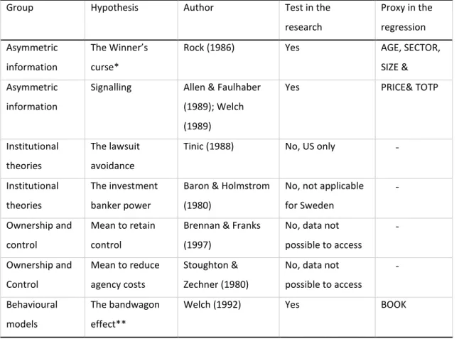
There exist several theories which can explain underpricing. However, there is no consensus regarding what causes underpricing or how to explain it in the scholar community. The traditional theories of underpricing suggested by Ritter (1998) and Ljungqvist (2004) have received the most attention in the IPO literature (Katto & Phani, 2016). The theories are grouped into four not mutually exclusive broad groups: asymmetric information models, institutional models, control models, and behavioral models which are described in Table 1 below:

Table 1. Overview of existing theories of underpricing

Group Hypothesis Author Test in the research Proxy in the regression Asymmetric information The Winner’s curse*

Rock (1986) Yes AGE, SECTOR, SIZE & Asymmetric

information

Signalling Allen & Faulhaber (1989); Welch (1989)

Yes PRICE& TOTP

Institutional theories

The lawsuit avoidance

Tinic (1988) No, US only _- Institutional

theories

The investment banker power

Baron & Holmstrom (1980)

No, not applicable for Sweden - Ownership and control Mean to retain control

Brennan & Franks (1997)

No, data not possible to access - Ownership and Control Mean to reduce agency costs Stoughton & Zechner (1980)

No, data not possible to access - Behavioural models The bandwagon effect**

Welch (1992) Yes BOOK

Source: (Ritter, 1998) (Ljungqvist, 2004)

(13)

The winner’s curse hypothesis

Rock (1986) introduced the theory which assumes some investors are better informed about the actual value of the shares in an IPO than the other investors in general. The informed investors can identify lucrative offers and mostly bid for attractive shares, and therefore receiving more of the attractive shares than the uninformed investors. Thus, less attractive firms underprice their issues to attract uninformed. Hence, “winning” an unattractive stock (Rock, 1986). Institutional investors are commonly regarded as informed, and data about bids from institutional investors are usually kept confidential, which limit the testable implication of this theory (Ljungqvist, 2004). Hence, proxies will instead be incorporated to test the Winner’s curse hypothesis. In accordance with previous studies, the following variables will be used; firm age (Ritter, 1991; Megginson & Weiss, 1990; Ljungqvist & Wilhelm, 2003), firm size (Ritter, 1991), and the sector which the company is active in (Ljungqvist & Wilhelm, 2003).

The age of a firm has been proven to have a negative relationship with the degree of

underpricing in an IPO, since investors are more uncertain about the future of younger firms. It is generally easier to estimate the value of an older firm due to the probable existence of more available information. Therefore, the information asymmetry should decrease with the increase in the age of a firm, because the market is more aware of the firm (Ritter, 1998; Durukan, 2002)

The Signalling hypothesis

Allen & Faulhaber (1989) and Welch (1989) have found support for the theory which assumes firms underprice their shares to signal good quality, since the appreciation of the shares on the first-day are considered to be a positive indicator about the firm’s quality. Although being costly for the firm due to the money forfeited, an underpricing may allow the firm to have a potentially better outcome in the event of a second offering.

The variable incorporated in the previous studies have generally been the offer price and the total listing period. A Firm with a lower offer price tends to record a higher level of

underpricing compared to an offer that has had a higher offer price (Fernando, et al., 1999). The total listing period indicates the time between the announcement of an IPO and the quoting day, and is also used to test for the signalling hypothesis. Quickly sold issues tend to be more underpriced because there exist less information in general. With a more extended subscription period, the potential investors may have more time to evaluate the prospect (Lee, Taylor & Walter, 1996; Ekkyokkya & Manpol, 2012).

(14)

The bandwagon effect hypothesis or Information Cascades

Welch (1992) introduced the theory which assumes the uninformed investors mimics the behaviour of the informed investor. In other words, the uninformed investor’s purchase and sell the same stocks like the informed investors. Thus, issuers underprice to encourage the informed investors to buy and induce a bandwagon effect in which more investors will follow (Ritter, 1998). As with the Winner’s curse, it is difficult to separate the investors from another which makes it complicated to test the theory. However, one may use book building as a proxy to distinguish between informed and uninformed investors. A dummy variable can be used to denote if the offer method was done with the Book building method as suggested by (Ljungqvist & Wilhelm, 2003; Ritter, 1984).

2.1.2 Theoretical explanations for long-run underperformance

There exist several theoretical explanations for the aftermarket underperformance of new issues, however, the most common and often cited in the IPO literature are the behavioural theories suggested by Ritter (1998): the divergence of opinion hypothesis, the impresario hypothesis, and the window of opportunity hypothesis.

The Divergence of Opinion Hypothesis

Introduced by Miller (1977) the theory assumes that when there is a high level of uncertainty about the valuation of an IPO, the buyers will be the most optimistic regarding the valuation of the firm. Consequently, the buyer’s valuation will be considerably higher than the pessimistic investors. As more information is known to the public, the uncertainty regarding the firms' future decreases. The difference of opinion between the optimistic and the pessimistic investors will diminish, causing the market price to drop accordingly (Ritter, 1998)

The Impresario Hypothesis or Fads Hypothesis

Shiller (1988) introduced the theory which assumes IPOs are subject to fads and that the underwriting firms deliberately underprice to generate more demand for the offer, making it a way to both promote the issuing and increase their reputation as underwriters. By deliberately underprice the issuing price, the underwriting firm creates a reputation of being successful taking firms to the market. From an investor point of view, this creates a high initial return, making it likely that investors will subscribe to their future IPOs. To deliberately underprice an IPO there is a necessity that there is a fad in the IPO market, meaning that investor optimism is high for IPOs. The underwriting firm gains a boost to their reputation by doing this.

(15)

in an IPO due to the difficulty to evaluate an IPO. Consequently, this hypothesis predicts that the firms with the highest initial return will have the lowest return in the longer-run. (Ritter, 1998)

The window of opportunity hypothesis

The hypothesis states that there are periods when the general public are optimism regarding the growth potential of firms going public. Consequently, firms will try to take advantage of this optimism by timing their IPO to that business cycle. During a business cycle with high optimism it is only natural that the volume of IPOs increases, however, the extent of the

increase seen cannot merely be explained by usual business cycle activity. The increase of firms is partially because some firms recognise an opportunity to receive more favourable terms regarding their IPO than what might be justifiable. Thus, firms going public in high volume periods are more likely to be overvalued (Ritter, 1998).

2.1.3 “Hot issue markets” phenomena

The HM phenomenon is considered to be an extension of the short-run underpricing phenomena (Ritter, 1991). The "hot issue" markets phenomena refer to period’s with general high initial return for IPOs, and with extensive underpricing throughout the IPO market. Furthermore, these periods tend to be followed by a rising volume of new IPO´s (Ritter 1998). Ibbotson & Jaffe (1975) found empirical evidence for periods when IPOs outperform their industry benchmark. Furthermore, Ritter (1984) documented the existence of a correlation between the "hot issue" periods and a large increase in the volumes of IPO´s, following these periods. However, during the time of increasing volumes, the initial returns were not as high as the peak of the prior hot issue period. Furthermore, if the market react positive for a firm, this may induce more

company’s within the same sector to go public earlier than planned because they want to partake in the hot market. The contrary may occur as well, when the market reacts negative.

(16)

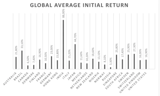
2.2 Previous studies on short-run underpricing

Numerous research have addressed the subject of underpricing in several markets and concluded new issues generally deliver high abnormal returns in the short run, Since the first evidence of IPO underpricing were presented by Stoll and Curley (1970), Logue (1973), and Ibbotson (1975). Logue (1973) and Ibbotson (1976) are pioneers of the IPO field and the first to use the term “underpricing”, while Rock (1985) and Baron (1980) were the first suggest potential explanations for the underpricing phenomena.Underpricing of IPO’s have been reported on national level and in different moments in time. Loughran, Ritter & Rydqvist (1994)

have summarised all the evidence of IPO underpricing since 1994, and maintains an updated IPO database. The average initial return for some selected countries are illustrated below in

Figure 1.

Figure 1. Average initial return for selected countries

Source: Adopted from Loughran et al. (1994, updated 2017)

21 ,8 0% 33 ,1 0% 6, 50 % 7, 40 % 16,9 0% 10 ,5 0% 23 ,0 0% 15 ,8 0% 88 ,0 0% 15 ,2 0% 44 ,7 0% 11 ,6 0% 10 ,2 0% 18,6 0% 13 ,1 0% 8, 10 % 3, 30 % 25 ,8 0% 17 ,4 0% ₂₅,9 0% 27 ,3 0% 16 ,0 0% 16 ,9 0%

(17)

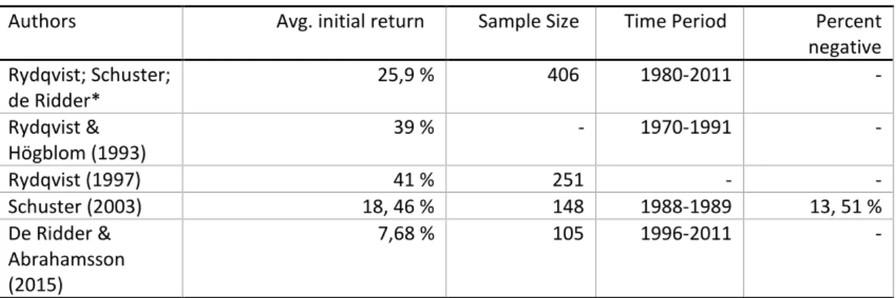
Evidence of underpricing in Sweden

The empirical evidence for underpricing on the Swedish market presented in below in Table 2:

Table 2. Empirical studies on short-run underpricing on the Swedish market

Authors Avg. initial return Sample Size Time Period Percent negative Rydqvist; Schuster; de Ridder* 25,9 % 406 1980-2011 - Rydqvist & Högblom (1993) 39 % - 1970-1991 - Rydqvist (1997) 41 % 251 - - Schuster (2003) 18, 46 % 148 1988-1989 13, 51 % De Ridder & Abrahamsson (2015) 7,68 % 105 1996-2011 -

* This figure was taken from (Loughran, et al., 1994)

2.3 Previous studies on long-run underperformance

Long-run underperformance of new issues was first suggested by Ibbotson (1975) and Ritter (1991) was the first to provide significant evidence that new issues underperformed. This encouraged other academics to research the field of IPO aftermarket performance on the

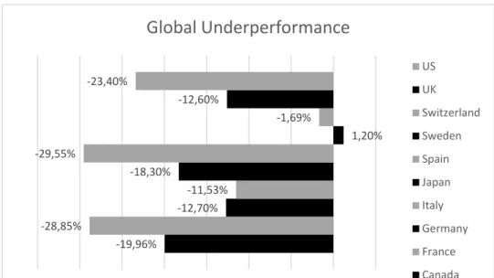
American market (Logue, 1973; Loughran & Ritter, 1995; Affleck-Graves & Spiess, 1995; Brav & Gompers, 2012). Aggarwal, Leal & Hernandez (1993) studied the Latin-American markets and proved that the anomaly existed outside the United States. Further, empirical research have later found the existence of the anomaly globally. The global evidence for some selected countries are presented in the section below.

(18)

Figure 2. Long-run aftermarket performance for selected countries

Studies in long-run aftermarket performance in Sweden

The studies conducted for the long-run underperformance on the Swedish market is presented below

Table 2. Swedish Studies in long-run underperformance

Authors Long-run performance Sample Size Time Period Method Loughran et al, (1994) 1,2 % 162 1980-2001 BHAR Westerholm (2006) 1,01 % 88 1994-2002 BHAR -19,96% -28,85% -12,70% -11,53% -18,30% -29,55% 1,20% -1,69% -12,60% -23,40% -35,00% -30,00% -25,00% -20,00% -15,00% -10,00% -5,00% 0,00% 5,00%

Global Underperformance

US UK Switzerland Sweden Spain Japan Italy Germany France Canada

(19)

Chapter 3: Method

3. Data Method & Methodology

This section will introduce the two methodologies used in the method, to answer the formulated research questions from the previous sections. The following sections will account for research strategy, the design of method, the process of data collection, data manipulation, data analysis, problems and weakness with the chosen method.

3.1 Introduction to method

This study examines the short-run and long-run market performance of Swedish IPO´s

undertaken during the period 2007-2017. The sample set will only include listings made on the Swedish stock markets Nasdaq Stockholm, Akitetorget and First North. The total dataset includes 229 observations from a population of 753 IPO´s in 2007-2017.

3.2 Research strategy

The adopted method for this investigation will be quantitative research with the deductive theory approach, which is in accordance to previous research. In other words, numerical values will be used to answer the research questions based on the theoretical framework. A quantitative research allows to measure the response from a respondent and facilitate the data into statistics for comparison, which is in alignment with the purpose of this thesis, measuring market performance for different sectors. The quantitative research starts with an analysis of related theories, from where the hypotheses are formed to investigate if there exists a relationship between selected variables. The hypotheses are empirically tested using statistical methods performed on a data sample, which are then confirmed or rejected (Bryman, 2012).

The other research strategy is the qualitative method, however, it is non-statistical and not suitable for this study (Yilmaz, 2013).

3.3 Research method

The research method is based on the approach suggested by Bryman (2012) who argues the following procedure is the ideal approach for a quantitative research. The following sections will present the research design and the data collection.

(20)

Chapter 3: Method

Building the theoretical framework

The literature examined was accessed from the electronics databases: IDEAS, Google Scholar, and Opus provided by the university. The keywords used to find literature

was: underpricing IPO, underperformance IPO, Sweden IPO, and sector IPO. To review the literature, the “association of business school academic journal quality guide” was used to determine the quality of the articles.

Development of hypothesis

From the research question and the theoretical framework the following hypothesis established.

Hypothesis 0: The market adjusted initial return short run performance (MAIR) is equal to zero Hypothesis 1: The market adjusted Initial return short run performance (MAIR) is not equal to zero

Hypothesis 0: The long−run performance (BHAR) is equal to zero Hypothesis 1: The long−run performance (BHAR) is not equal to zero

Research design

This research will have two designs since the characteristics of the research question are different. The descriptive design aims to describe a particular situation or phenomena and was adopted for RQ1 & 3 since the aim is to answer if underpricing and underperformance exist on the Swedish markets in different sectors (Bryman, 2012).

An explanatory research design aims to explain a relationship between two variables, and was adopted for RQ2 since the aim is to explain some determinants for the underpricing

phenomena’s (Bryman, 2012).

Devise measurement of concepts

A concept in the quantitative research strategy is building blocks from the theory and represent the central point on which around the research is conducted. A concept has to be measured, usually in the form of a dependent and independent variable, and then compared against an indicator. In other words, theories may explain a particular phenomenon (Bryman, 2012). This investigation will use a regression model where the dependent variables are the calculation of underpricing, while the independent variables are based on the existing literature. The output from the statistical analysis were compared against an indicator, the OMX 30.

(21)

Chapter 3: Method

Sample selection

From January 2007 to December 2017, 751 firms went public on the three Swedish stock markets. Thus, the IPO population for the study consisted of a total 751 observations. The intention was to have the largest sample possible to eliminate the effect of fluctuating market conditions, as well as to include tops and bottoms in the IPO waves in the most accurate way. 229 observations remained after the elimination of IPO’s. The criteria were; lack of financial information (data), name changes after an IPO, transfers between lists, foreign IPO´s, secondary listings, transfers from other stock exchanges in Sweden, spin-offs, offers targeted to individual investors, de-listings, and M & A.

Sector classification

Sectors will be classified after the Bloomberg Industry Classification (BIC), which is commonly used on the Swedish stock market. Kim & Ritter (1999) used the Standard Industry

Classification (SIC) in their paper, however, argueslon BIC is a better sector classification system since SIC classify firms after which product they produce. Hence, it is challenging to classify multiproduct firms, and some firms have been wrongly classified (Kim & Ritter, 1999).

Collection of data and research instruments

For this study, secondary sources provided the data. The website nyemissioner.se provided the list of IPO’s in-between 2007-2017. Datastream provided the return for each IPO and the OMX30. The offer price (PRICE), firm age (AGE), Revenue (SIZE), and book building were retrieved from each firms prospectus. The data were processed in the software Excel and the statistical program SPSS. Furthermore, NASDAQ, the Swedish Tax Agency, and annual reports were used as a complement for finding missing information.

(22)

Chapter 3: Method

3.4 Methodology on short-run underpricing

Short-run initial market performance will be measured using the first-day return and will follow the standard methodology developed by Logue (1973) and Ritter (1984) to be consistent with previous studies.

3.4.1 Calculation of the first-day return

The initial return is defined as the percentage of the price change from the offering price and closing share price at the end of the first trading day. Initial returns (IR) and Market Adjusted initial Returns (MAIR) are the two most common methods to calculate the first-day returns. Both measurements will yield a similar result and are not statistically significant different, however, MAIR will account for the market movements of the selected benchmark (Ljungqvist & Wilhelm, 2003). Logue (1973) argues that MAIR measure underpricing more correct since IR does not account for the market movements.

To adjust for market movements the IR are subtracted by corresponding return of OMX30.

𝑀𝑀𝑀𝑀𝑀𝑀𝑀𝑀= 𝑀𝑀𝑀𝑀 − 𝑀𝑀𝑀𝑀 = 𝑃𝑃𝑖𝑖,1_𝑃𝑃− 𝑃𝑃𝑖𝑖,𝑜𝑜 𝑖𝑖,𝑡𝑡−1 − 𝑂𝑂𝑀𝑀𝑂𝑂𝑂𝑂301− 𝑂𝑂𝑀𝑀𝑂𝑂𝑂𝑂300 𝑂𝑂𝑀𝑀𝑂𝑂𝑂𝑂30𝑜𝑜 (1) Where:

𝑀𝑀𝑀𝑀𝑀𝑀𝑀𝑀 = Market adjusted initial return of company i at time 1 𝑃𝑃𝑖𝑖,0= the first-day opening price for company i

𝑃𝑃𝑖𝑖,1 = The first-day closing price for company i 𝑂𝑂𝑀𝑀𝑂𝑂𝑂𝑂300 = The first-day opening price for OMXS30 𝑂𝑂𝑀𝑀𝑂𝑂𝑂𝑂301= The first-day closing price for the OMXS30

If the IPO’s are underpriced the initial return are greater than zero (+ %), and if underpriced the MAIR are below zero (- %). After calculating the first-day return a t-statistics test was used to test if the first-day returns are statistically significant.

3.4.2 Testing for statistical significance

After the calculation of the MAIR for each firm according to the calculation above the next step is to determine if the result is statistically significant. The sample were not normal distributed and therefore a non-parametric test was used (Gujarati, 2003).

(23)

Chapter 3: Method

One sample student’s t-test

The statistical method of a student t-test was conducted to examine the average level of underpricing for Swedish IPO´s and for each sector. The t-test analyse the significance and wheatear to accept or reject the null hypothesis using the following formula:

𝑡𝑡 =𝑂𝑂� − 𝜇𝜇 𝑂𝑂/√𝑛𝑛

(2)

Where:

𝑂𝑂� = the sample mean

𝜇𝜇 = the value that gives the lowest possibility to reject the null hypothesis 𝑂𝑂 = the sample standard deviation

𝑛𝑛 = the number of observations in the sample

Independent sample student’s t-test

An independent sample student’s t-test will determine if there exist a difference for the average MAIR between different sectors using the following formula:

𝑡𝑡 = (𝑥𝑥�� − 𝑥𝑥1 ��)2 �𝑂𝑂𝑝𝑝2 𝑛𝑛1+ 𝑠𝑠𝑝𝑝2 𝑛𝑛2 (3) Where:

𝑂𝑂1𝑂𝑂2= Sample mean for two population 𝑛𝑛1𝑛𝑛2 = Observations for two populations 𝑂𝑂𝑝𝑝2𝑂𝑂𝑝𝑝2= Standard deviation for two populations

3.4.3 Multiple regression model - ordinary least squares (OLS)

A multiple regression model will examine wheatear the selected theories can explain the degree of underpricing, and six explanatory variables will be incorporated into the OLS, which were picked based on the theoretical framework to hopefully explain some part of the relationship between the factors affecting underpricing. The method of Ordinary Least Squares (OLS) is the most common statistical technique for analysing IPO underpricing, and it have has used

(24)

Chapter 3: Method

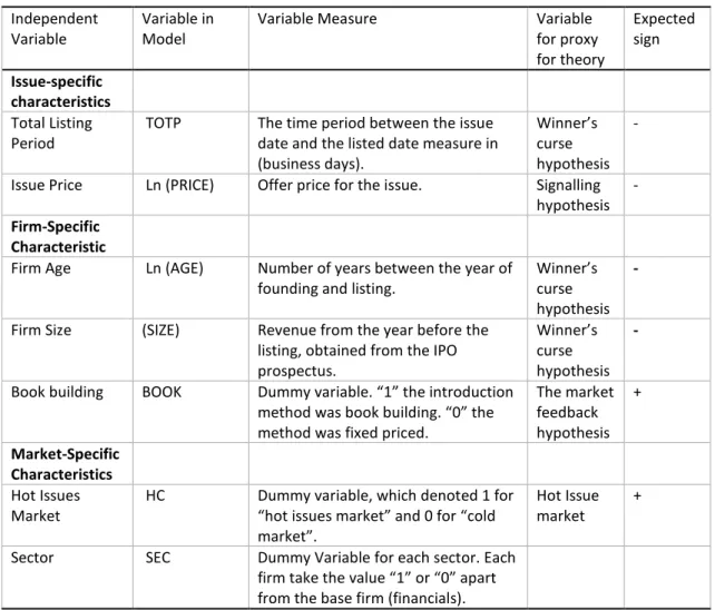
Table 4. Independent variables with measurement, expected sign and relevant theories.

Independent

Variable Variable in Model Variable Measure Variable for proxy for theory Expected sign Issue-specific characteristics Total Listing

Period TOTP The time period between the issue date and the listed date measure in (business days).

Winner’s curse hypothesis

- Issue Price Ln (PRICE) Offer price for the issue. Signalling

hypothesis -

Firm-Specific

Characteristic

Firm Age Ln (AGE) Number of years between the year of

founding and listing. Winner’s curse hypothesis

-

Firm Size (SIZE) Revenue from the year before the listing, obtained from the IPO prospectus.

Winner’s curse hypothesis

-

Book building BOOK Dummy variable. “1” the introduction method was book building. “0” the method was fixed priced.

The market feedback hypothesis + Market-Specific Characteristics Hot Issues

Market HC Dummy variable, which denoted 1 for “hot issues market” and 0 for “cold market”.

Hot Issue market + Sector SEC Dummy Variable for each sector. Each

firm take the value “1” or “0” apart from the base firm (financials).

(25)

Chapter 3: Method

Development of hypothesis for the independent variables

The Total listing Period (TOTP):

Hypothesis 0: There is no association between the level of underpricing and the TOTP of the issuing firm

Hypothesis 1: There is a negative association between the level of underpricing and the TOTP of the issuing firm

The issue price (PRICE):

Hypothesis 0: There is no association between the level of underpricing and PRICE of the issuing firm.

Hypothesis 1: There is a negative association between the level of underpricing and the PRICE of the issuing firm.

The Firm Age (AGE):

The proxy for firm age is calculated after the approach by (Ritter, 1991).

𝐹𝐹𝑖𝑖𝑟𝑟𝑚𝑚 𝑎𝑎𝑎𝑎𝑎𝑎= ln( 1 + (𝑖𝑖𝑠𝑠𝑠𝑠𝑖𝑖𝑎𝑎 𝑦𝑦𝑎𝑎𝑎𝑎𝑟𝑟 − 𝑓𝑓𝑖𝑖𝑟𝑟𝑚𝑚 𝑓𝑓𝑜𝑜𝑖𝑖𝑛𝑛𝑓𝑓𝑖𝑖𝑛𝑛𝑎𝑎 𝑦𝑦𝑎𝑎𝑎𝑎𝑟𝑟)) (4)

Hypothesis 0: There is no association between the level of underpricing and the AGE of the issuing firm

Hypothesis 1: There is a negative association between the level of underpricing and the AGE of the issuing firm.

The firm size (SIZE):

Hypothesis 0: There is no association between the level of underpricing and the SIZE of the issuing firm

Hypothesis 1: There is a negative association between the level of underpricing and the SIZE of the issuing firm.

Hot issue Markets (HC)

Hypothesis 0: There is no association between the level of underpricing and the volume of IPO’s

Hypothesis 1: There is a positive association between the level of underpricing and the volume of IPO’s

(26)

Chapter 3: Method

Book building (BOOK)

Hypothesis 0: There is no association between the level of underpricing and the introduction method of the firm

Hypothesis 1: There is a positive association between the level of underpricing and the introduction method of the firm

Regression

The following regression analysis was used to analyse:

𝑀𝑀𝑀𝑀𝑀𝑀𝑀𝑀= 𝛼𝛼 +�𝛽𝛽_𝑗𝑗𝐷𝐷𝑖𝑖,𝑗𝑗+ 𝜀𝜀𝑖𝑖 𝑚𝑚

𝑗𝑗=1

(5)

Where:

Ri,= Short run returns

βi=Coefficient of the explanatory variables Di,j=explanatory variable

εi=the error term of the model

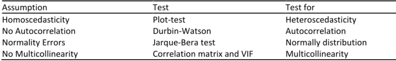
Diagnostics test for the regression analysis - OLS assumptions

Since the studies is based on cross-sectional data, four potential violations of the classical linear regression Model (CLRM) were examined to established a valid regression model and fulfil the Markov theorem. The assumptions are presented in the table below:

Table 3. Assumption in the OLS regression

Assumption Test Test for

Homoscedasticity Plot-test Heteroscedasticity No Autocorrelation Durbin-Watson Autocorrelation Normality Errors Jarque-Bera test Normally distribution No Multicollinearity Correlation matrix and VIF Multicollinearity

Plot test for heteroscedasticity

A linear regression is always assumed to have homoscedasticity, while if heteroscedasticity is present, the variance of the error terms is systematic which implies others estimators could provide a better-fitted line, and therefore the OLS analysis would not be reliable. Performed through visually judging the distribution shape of the scatterplot for the dependent variable, where the Y-axis consists of the regression standardised residuals while the X-axis consists of the regression standardised predicted value. If there exist heteroscedasticity the scatter plot will

(27)

Chapter 3: Method

have a cone-shaped distribution, starting narrow from the left and after that widening (Rosopa, Schaffer & Schroeder, 2013).

If there is a doubt that there might exist a cone-shaped distribution, a Mann–Whitney

heteroscedasticity test can be performed. Furthermore, two examples of scatterplots displaying homoscedasticity and heteroscedasticity are attached in Appendix 3.

Durbin-Watson test for autocorrelation

If the data set is considered to be autocorrelated, the errors of adjacent observations are

correlated, which could underestimate the standard error of the coefficients. The Durbin-Watson test determines wheatear the correlations adjacent error terms is equal to zero. The Durbin-Watson statistics are calculated in SPSS and is between 0-4, a value above two indicates there is no autocorrelation in the dataset. Although, the standard practice is to accept values which are in the range of 1, 5 -2, 5, since these values are relatively normal. Values outside this range should be a cause for concern (Gujarati, 2003).

Jarque-Bera test for normally distribution errors.

A normally distributed sample need to pass two criteria: no skewness because it is a measure to which extent a distribution is symmetrical around the mean for the sample and a coefficient kurtosis of 3 which is a measure of the size of the tails in the distribution. To determine the normal distribution, the histogram over the distribution will be examined, and a Jarque-Bera test will be conducted. The test rejects the null hypothesis at the 5 percent level. The null hypothesis is:

Hypothesis 0: the error terms are normal distributed Hypothesis 1: the error terms are not normal distributed

The Jarque-Bera statistics are calculated after the following formula:

𝐽𝐽𝐽𝐽 = 𝑛𝑛_{6 (𝑂𝑂}2₊(𝑘𝑘 − 3)2

4 )

(6)

Where:

𝑛𝑛 = the sample size 𝑠𝑠 = the sample Skewness 𝑘𝑘 = the sample kurtosis

(28)

Chapter 3: Method

Correlation matrix and VIF for multicollinearity

When testing for multicollinearity in the independent variables the common practice is to use 0, 7 or 0, 8 as a maximum Value, meaning if the correlation between two independent variables are above it, Collinearity is likely to exist. Furthermore, if the correlation is above 0, 8 collinearity is most likely to exist. To examine multicollinearity, a Pearson correlation matrix from the regression output as well as a regular correlation matrix was tested.

3.5 Methodology on long-run underperformance

Two approaches are commonly employed in the IPO literature for calculating long-run abnormal returns: ETIME and the calendar time approach (CTIME). For each approach, two methodologies can be adapted to measure the after-market performance, which makes it possible to utilise four techniques for measuring long-run abnormal return. The two methods in the ETIME approach are the Buy-and-hold method (BHAR) and the Cumulative Abnormal Return (CAR) method. Furthermore, the CTIME approach consists of two methods as well, the Yearly Calendar-time Abnormal Returns (YCTAR) and the Fama-French three-factor

regression.

Motivated by the existing international practice, long-run abnormal returns were calculated using the Event-time approach (ETIME) with the Buy-and-hold method (BHAR), developed by Ritter (1991) and used by Westerholm (2006). The use of BHAR provides the opportunity to compare the results to previous research since it is the most widely used. The ETIME approach compute returns after a specific event, in this case, the month after the listing date to exclude the underpricing effect. The returns will be calculated on a monthly basis for a long-time horizon which is 3 years (36 months), in accordance with previous research. Ritter (1991) found that after 3 years the effect of the aftermarket underperformance diminishes. The returns for each IPO are bundled together to create a portfolio which is then measured against a selected

benchmark. The ETIME approach has been criticised by Mitchel and Stafford (2000), and Fama (1998) since the ETIME can overstate the statistical significance of the abnormal returns

because of cross-sectional independence of the observations.

BHAR vs CAR

CAR is computed by summing of the mean benchmark-adjusted returns for a specific interval following the issuance day until the end of the period. BHAR was selected over CAR for two reasons: 1) BHAR better reflect what the investors would get in return.2) It is the most accepted

(29)

Chapter 3: Method

The main difference between the two models is that BHAR takes into consideration the

compounding effect while CAR disregards it. The returns for an investor is better approximated by the compounding effect because it better simulates an investor’s portfolio. Hence, BHAR is the preferred method because CAR does not adequately measure the returns obtained by an investor. However, CAR has been proven to be more statistically significant to determine if abnormal returns are positive or negative compared to the benchmark. CAR is also less likely to lead to a false rejection of the market efficiency Fama (1998).

Buy-and-hold abnormal returns (BHAR)

The buy and hold abnormal returns (BHAR) method mimics an investment strategy where the investor buy shares and hold them for a certain time-period. BHAR is the abnormal return calculated by deducting the monthly return from the benchmark return (Barber & Lyon, 1997). The BHAR is calculated in three steps starting with the monthly returns for each firm, and then the return for the OMXS30 are subtracted. The last step of the BHAR calculations is to calculate an aggregated geometric mean BHAR for the sample group with equal weights, illustrated in the equations below. 𝑀𝑀𝑖𝑖,𝑡𝑡= 𝑃𝑃1_𝑃𝑃− 𝑃𝑃0 0 (7) Where

𝑟𝑟𝑖𝑖,𝑡𝑡 =Monthly return for each firm 𝑃𝑃1= Price of the start of the month 𝑃𝑃0= Price at the end of the month

The return for the OMSX30 are then subtracted: 𝐽𝐽𝐵𝐵𝑀𝑀𝑀𝑀𝑖𝑖,𝑡𝑡= � (1 + 𝑟𝑟𝑖𝑖,𝑡𝑡) 𝑇𝑇 𝑡𝑡=36 − � (1 + �𝑂𝑂𝑀𝑀𝑂𝑂𝑂𝑂30𝑖𝑖,𝑡𝑡�) 𝑇𝑇 𝑡𝑡=36 (8) Where:

𝑟𝑟𝑖𝑖,𝑡𝑡= Monthly return for each firm 𝐸𝐸𝑟𝑟𝑖𝑖,𝑡𝑡 =Monthly return for OMSX30

After calculating the BHAR, the returns are then bundled together to create an average for the study period:

(30)

Chapter 3: Method 𝐽𝐽𝐵𝐵𝑀𝑀𝑀𝑀36 �� = � 𝑤𝑤𝑖𝑖𝐽𝐽𝐵𝐵𝑀𝑀𝑀𝑀𝑖𝑖,𝑡𝑡 229 𝑖𝑖=1 (9) Where: 𝑤𝑤𝑖𝑖 =1_𝑛𝑛 Reference portfolios

The BHAR methodology requires a benchmark to assess the relative aftermarket performance to eliminate the biases which are associated with long-run event studies. This is commonly solved by creating several reference portfolios, with firm size and market to book ratio as key numbers for optimising the comparison (Barber, Lyon & Tsai, 1999). However, in this study solely the OMXS30 index will be integrated as a benchmark. This is mainly due to the size of the Swedish stock market because there are not enough appropriate firms to be combined into the reference portfolios. Furthermore, the amount of time available for this study would not be enough to create the reference portfolios.

Value-weighted or equally-weighted BHAR

Value-weighted BHAR: If the interest is to quantify the change in the average wealth of the

investor as a consequence of a certain event, the correct method would be the valued weighting approach. This method requires the number of shares for each issue. However, this would result in a measurement problem since the number of shares in an IPO is not always decided before the introduction, it often depends on the demand of the IPO. Because of this, more observations would have had to be discarded, which would have reduced the sample size further.

Equally-weighted BHAR: if the interest lies in the implications of a potential stock market

mispricing, a method based on equally weighted returns would be more appropriate. Thus, corresponding with the purpose of this thesis. Furthermore, since it did not require the number of shares more observations could be included in the sample.

(31)

Chapter 3: Method

Statistical test for the buy-and-hold abnormal returns

To validate the long-run performance return produced by the BHAR empirically, we will test this papers null hypothesis with a conventional T-statistic. The following section will follow Barber, et al. (1999) tests to evaluate the BHAR. The first step is to perform a conventional T-test: 𝑡𝑡 = 𝐽𝐽𝐵𝐵𝑀𝑀𝑀𝑀��𝑇𝑇 𝜎𝜎(𝐽𝐽𝐵𝐵𝑀𝑀𝑀𝑀𝑇𝑇)/√𝑛𝑛 (10) Where: 𝐽𝐽𝐵𝐵𝑀𝑀𝑀𝑀𝑇𝑇

�� = the sample mean

𝜎𝜎(𝐽𝐽𝐵𝐵𝑀𝑀𝑀𝑀𝑇𝑇)/√𝑛𝑛 = the cross-sectional sample standard deviation of the sample consisting of n firms.

Barber and Lyon (1997) documented that the Buy and Hold abnormal returns are positively skewed and that this leads to a negatively biased t-statistics. To eliminate the skewness bias, this study will use Barber et al. (1999) proposed use of a bootstrapped skewness-adjusted t-statistic:

𝑡𝑡𝑠𝑠𝑠𝑠 = √𝑛𝑛(𝑂𝑂 +1_{3 𝑦𝑦�𝑂𝑂}2+_{6𝑛𝑛 𝑦𝑦�}1 (11) Where

𝑂𝑂 =

𝐵𝐵𝐵𝐵𝐵𝐵𝐵𝐵��𝑇𝑇 𝜎𝜎(𝐵𝐵𝐵𝐵𝐵𝐵𝐵𝐵𝑇𝑇), and

𝑦𝑦� =

∑𝑛𝑛𝑖𝑖=1(𝐵𝐵𝐵𝐵𝐵𝐵𝐵𝐵𝑖𝑖𝑇𝑇−𝐵𝐵𝐵𝐵𝐵𝐵𝐵𝐵��𝑇𝑇)3 𝑛𝑛𝜎𝜎(𝐵𝐵𝐵𝐵𝐵𝐵𝐵𝐵𝑇𝑇)3 𝑦𝑦� =The coefficient of skewness.

(32)

Chapter 4: Empirical Results

4. Empirical Results

This section will account for the findings in the research which includes the short-run and long-run returns for the IPO’s, the statistical test for significant and the output from the regression analysis.

4.1 Results for the short-run market performance

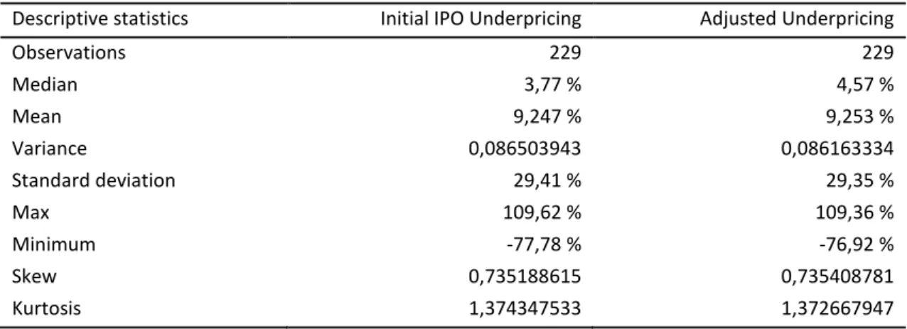
4.1.1 Descriptive statistics

The sample of 229 IPO’s from a population of 751 in-between 2007-2017 resulted in an IR of 9,247 % which is the arithmetic average return of the unadjusted IR on the Swedish equity market. When adjusting for the market movements, the underpricing amounts to 9,253 %, which is a slight increase compared to the unadjusted returns. Table 4 below summarises the

descriptive results for the observed post-day results.

Table 4. Descriptive statistics of post day returns

Descriptive statistics Initial IPO Underpricing Adjusted Underpricing

Observations 229 229 Median 3,77 % 4,57 % Mean 9,247 % 9,253 % Variance 0,086503943 0,086163334 Standard deviation 29,41 % 29,35 % Max 109,62 % 109,36 % Minimum -77,78 % -76,92 % Skew 0,735188615 0,735408781 Kurtosis 1,374347533 1,372667947

The average underpricing is slightly higher in the adjusted Method, indicating the average IPO stock price increased by 9,253 % at the end of the first-day trading. The skewness of 0, 7354 for the adjusted underpricing indicates the distribution of the sample has a long right tail, meaning the sample´s distribution is skewed to the right. Together with kurtosis of 1, 37 the measurement of symmetry indicates the sample is not normally distributed. The highest adjusted underpricing for a firm in the sample was 109, 36 %, and the lowest was -76, 92%.

(33)

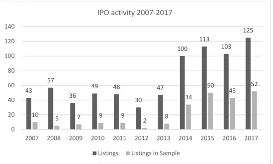
Sample set of IPOs in the short run

Figure 3 illustrates the IPO activity on a yearly basis for the IPO’s introduced on the Swedish stock market of Nasdaq Stockholm, First North and Aktietorget. The sample consist of 229 observations which has been vetted according to the sample criteria’s for the sample selection.

Figure 3. IPO activity 2007-2017

Panel A Panel B 43 57 36 49 48 30 47 100 113 103 125 10 ₅ ₇ 9 9 2 8 34 50 43 52 0 20 40 60 80 100 120 140 2007 2008 2009 2010 2011 2012 2013 2014 2015 2016 2017 IPO activity 2007-2017

Listings Listings in Sample

10 5 7 9 9 ₂ 8 34 50 43 52 0 10 20 30 40 50 60 2007 2008 2009 2010 2011 2012 2013 2014 2015 2016 2017

Sample IPO's per year

(34)

Panel A illustrates all the IPO’s issued on the three Swedish stock markets 2007-2017 and the observations which meet the criteria’s to be included in the sample. Panel B illustrates the sample distribution on a yearly basis more precise. The visual inspection of the two graphs depicts a similar pattern which indicates that the distribution does not change significantly after eliminating observations. The latest four years have seen a substantial increase in the number of IPOs listed compared to the earlier six years of the study period. The year with the lowest number of IPOs who were accepted was 2012, where just two IPOs qualified for the sample. The year with the most qualified IPOs was 2017 with 52 IPOs closely followed by 2015 with 50 IPO’s.

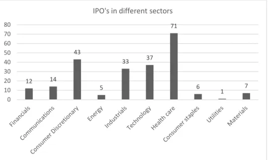
Figure 4. Distributions of IPO in different sectors

The chart above depicts the distribution of IPOs for each sector, classified according to the Bloomberg Industry Classification (BIC). There are four prominent sectors which made up of a significant part of the sample; Consumer Discretionary, Industrials, Technology, and Health Care. The sectors with the lowest amount of IPOs is the Utility sector with only 1 IPO, followed by the Energy sector with five.

12 14 43 5 33 37 71 6 1 7 0 10 20 30 40 50 60 70 80

(35)

4.1.2 Tests for statistical significance

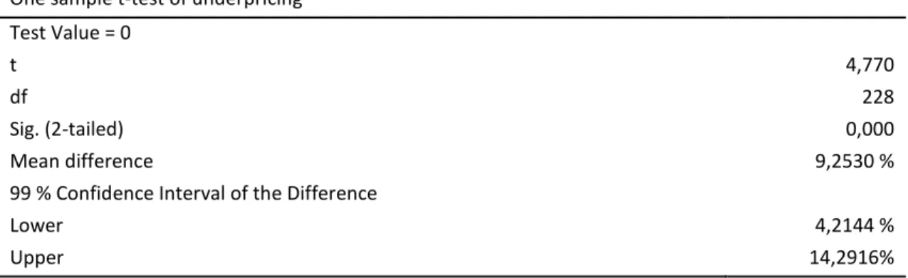
One Sample Student t-test

Table 5. One Sample Student t-test

One sample t-test of underpricing Test Value = 0

t 4,770

df 228

Sig. (2-tailed) 0,000

Mean difference 9,2530 %

99 % Confidence Interval of the Difference

Lower 4,2144 %

Upper 14,2916%

The two-tailed one sample student T-test has a significance of 0,000, which rejects the null hypothesis on the 1 % significance level, confirming with a statistical significance that the underpricing in Sweden is not equal to zero.

(36)

Descriptive statistics for sectors

Figure 5. Average underpricing per sector

Table 6. Descriptive statistics for sectors

Sector IPO's avg MAIR Underpriced firms median st.dev t-stat Significance

Industrials 33 20,77 % 73 % 17,08 % 32,4 % 3,684 0,001 Technology 37 11,85 % 65 % 6,00 % 29,2 % 2,47 0,018 Materials 7 10,12 % 71 % 3,86 % 22,1 % 1,209 0,272 Consumer Discretionary 43 9,79 % 63 % 10,06 % 26,1 % 2,456 0,018 Health Care 71 8,96 % 55 % 2,90 % 33,1 % 2,28 0,026 Financials 12 4,89 % 75 % 2,94 % 6,2 % 2,715 0,02

Utilities 1 – 1,98 % 0 % – 1,98 % N/A N/A N/A

Communications 14 – 5,42 % 36 % – 6,16 % 22,0 % – 0,922 0,373

Energy 5 – 10,05 % 60 % 0,75 % 22,5 % – 0,999 0,374

Consumer Staples 6 – 10,55 % 33 % – 11,30 % 23,9 % – 1,08 0,329

Table 6 above summarise the statistics for each sector. The sector with the highest average underpricing (MAIR) is the Industrials sector with 20, 77 %, followed by the Technology sector with 11, 85 %. Further, the sector with the highest overpricing is the consumer staples sector followed by the Energy sector. The percentage of underpriced IPOs for each sector is the highest in the financial sector with 75 %, closely followed by the Industrials sector with 73 %.

11,85% -5,42% 9,79% -10,05% 8,96% 20,77% -10,55% -1,98% 4,89% 10,12% -20,00% -10,00% 0,00% 10,00% 20,00% 30,00%

Average underpricing per sector

Materials Financials utilities Consumer Staples Industrials Health Care Energy Consumer Discretionary Communications Technology

(37)

dispersed the values in each sector is from the mean. The financial sector has the lowest standard deviation of 6, 2 %, indicating that there are no major outliers in the sector. However, an important aspect is the significance of each sector. Further, when using a significance level of 0, 05, there is only five out of the ten sectors which can be considered statistically significant. The sectors which were statistically significantly different from zero where: Industrials,

Technology, Consumer Discretionary, Health Care and Financials.

4.1.3 Multiple regression analysis Table 7. Multiple regression output.

Regression

R 0,366

R Square 0,134

Adjusted R Square 0,073

Std. Error of the Estimate 28,27 %

Durbin-Watson 1,903

The multiple regression analysis calculated the R square value which explains the goodness of fit of the regression model, which is the regression was made on the sample of 229 IPOs amounts to 0,134. Furthermore, the regression analysis derives the Durbin-Watson value for the sample set. The Durbin-Watson value of 1,903 is below 2. However, it is above 1, 5 and the assumption made is that no autocorrelation exists in the data sample based on the common practice to accept values in the range 1, 5 – 2, 5.

Statistics of Independent variables

Table 8 illustrate the t-statistic and the statistical significance for each of the independent variable used in the multiple regression analysis. Of the six variables, only the variable for the total listing period (TOTP) was statistically significant on the 5% significance level. Further, the offer price (PRICE) and the hot and cold market (HC) variables were the two who were the closest to be significant of the other five. The HC and BOOK were dummy variables in the regression.

(38)

Table 8. Statistics of Independent variables

Variable t-statistic Significance

AGE 0,048 0,962 TOTP -3,701 0,000 SIZE -0,049 0,961 PRICE -1,620 0,107 HC 1,527 0,128 BOOK -0,917 0,360 Regression Diagnostics Jarque-Bera test

The Jarque-Bera test is as earlier explained using a hypothesis for evaluating the result with a 0, 05 significance level for the P-value. Hence, the P-value of 0,001 from the Jarque-Bera

performed on the sample indicates that we reject the hypothesis that the sample is normally distributed. The null hypothesis are rejected at 5 % significant level which indicates that the sample of 229 IPOs is not considered to have a normal distribution. Since the distribution was not normally distributed, it is justified using non-parametric methods which works better with non-normal distributions.

Table 9. Jarque-Bera test

Determinant Value Correct

Skewness 0,735409 0

Kurtosis 1,372668 3

(39)

Figure 6. Histogram for dependent variable

The visual inspection of the distribution also indicates the distribution is not normally distributed, however, this approach cannot be guaranteed. Nonetheless, a non-normal

distribution can be disregarded according to the central limit theorem. Since the sample used in this paper is 229 IPO´s, the non-normality of the sample is ignored due to the size of the sample.

Heteroscedasticity

Figure 7 below contain the scatterplot that one use to visually asses weather the sample set possess qualities of homoscedasticity or heteroscedasticity. When reviewing the distribution of the sample set one can identify clear indicators of homoscedasticity, since it do not follow any clear pattern or possess any indication of a cone shaped distribution. Further, the overall shape of the distribution possess indicators of non-random clustering. Hence, one may visually verify that the assumption of that homoscedasticity is present, is correct.

(40)

Figure 7. Heteroscedasticity

Multicollinearity

Table 10. Correlation Matrix

Correlation Matrix SIZE TOTP AGE PRICE

SIZE 1

TOTP – 0,347 1

AGE 0,378 – 0,428 1

PRICE 0,443 – 0,631 0,439 1

The values of the correlation coefficient between the independent variables do not exceed the critical value of 0, 8. The highest correlation between two independent variables is as illustrated above, the correlation between PRICE and SIZE with a value of 0,443. Hence, there exist no multicollinearity in the data sample set.

(41)

4.2 Results for the long-run market performance 4.2.1 Descriptive statistics

Table 11 illustrates the results obtained when using the ETIME approach with the BHR and

BHAR methods in a three-year horizon. Table 12 illustrates the long-run return for different sectors.

Table 11. 3-year buy and hold abnormal returns for Swedish IPO

Descriptive statistics BHAR

Observations 86 Ave. Return 2,68 % Median -12,98 % Variance 73,92 % Standard deviation 85,98 % Max 348,33 % Minimum -166,27 %

Table 12. Long-run return for different sectors

Sectors Sample size Average BHA Average BHAR Median Maximum Minimum Utilities 1 -53,44 % -68,22 % -68,22 % -68,22 % -68,22 % Financials 5 -16,66 % -37,75 % -74,94 % 50,13 % -113,29 % Energy 2 -37,94 % -36,56 % -36,56 % 3,23 % -76,35 % Consumer Staples 3 -21,61 % -32,11 % -36,04 % -1,81 % -17,58 % Materials 4 17,19 % -25,00 % -28,43 % 60,25 % -103,39 % Communications 7 -4,34 % -16,09 % -17,58 % 113,50 % -166,27 % Technology 9 2,03 % -7,36 % -42,10 % 126,12 % -87,44 % Consumer Discretionary 17 13,12 % 4,68 % 15,86 % 97,13 % -89,66 % Industrials 14 21,65 % 7,22 % -39,57 % 348,33 % -80,32 % Health Care 24 51,95 % 31,44 % 26,92 % 228,96 % -105,43 %

The average BHA is the three-year returns for each sample before taking into account the benchmark returns, while the average BHAR is when the benchmark returns have been subtracted from the samples three-year returns. The use of buy and hold returns to estimate the long-run market performance of Swedish IPO reveals the non-existence of underperformance after 3-years and an over performance of 2,68 %. Three sectors outperformance the Swedish market: health care, industrials and consumer discretionary, which were also the most active sectors on the Swedish market. The sectors that underperform have quite small sample sizes, larger samples would be needed in each sector to increase the comparability.

(42)

Distributions of IPO’s

Figure 8 illustrates the number of IPO which met the criteria’s to be incorporated in the

research fluctuates over the study period, being the highest in 2014 with 34 IPO´s.

Figure 8. Long-run IPO Activity

One Sample Student t-test

The results from the One-Sample Student t-test to test whether Swedish IPO underperform in the long-run are illustrated below:

Table 13. One sample t-test for underperformance

One sample t-test of underperformance Test Value = 0

t 0,289

df 85

sig. (2-tailed) 0,774

Mean difference 0,026761

95 Confidence interval of the difference

Lower -0,15757

Upper 0,2111

The t-test was performed on the full sample for the long-run IPO´s, with 86 IPO´s. The results are that t is equal to 0,289 and the significance of the test is 0,774 and accepts the hypothesis of the long-run performance, indicating that IPO´s do not underperform in a three year period

10 5 7 9 9 2 8 34 2 0 5 10 15 20 25 30 35 40 2007 2008 2009 2010 2011 2012 2013 2014 2015