Postprint
This is the accepted version of a paper published in Journal of Chemical Physics. This paper has been
peer-reviewed but does not include the final publisher proof-corrections or journal pagination.
Citation for the original published paper (version of record):
Ahlstrand, E., Zukerman Schpector, J., Friedman, R. (2017)
Computer simulations of alkali-acetate solutions: Accuracy of the forcefields in difference
concentrations.
Journal of Chemical Physics, 147: 1-10
https://doi.org/10.1063/1.4985919
Access to the published version may require subscription.
N.B. When citing this work, cite the original published paper.
Permanent link to this version:
in difference concentrations
Emma Ahlstrand,1Julio Zukerman Schpector,2and Ran Friedman1, a)
1)
Linnæus University, Department of Chemistry and Biomedical Sciences, Linnæus University, 391 82 Kalmar, Sweden
2)Universidade Federal de S˜ao Carlos, Departamento de Qu´ımica, CP 676, 13565-905 S˜ao Carlos, SP,
Brazil
(Dated: 24 October 2017)
When proteins are solvated in electrolyte solutions that contain alkali ions, the ions interact mostly with carboxylates on the protein surface. Correctly accounting for alkali-carboxylate interactions is thus impor-tant for realistic simulations of proteins. Acetates are the simplest carboxylates that are amphipathic, and experimental data for alkali acetate solutions is available and can be compared with observables obtained from simulations. We carried out molecular dynamics simulations of alkali acetate solutions using polarizable and non-polarizable forcefields, and examined the ion-acetate interactions. In particular, activity coefficients and association constants were studied in a range of concentrations (0.03, 0.1, and 1 M). In addition, quantum-mechanics (QM) based energy decomposition analysis was performed in order to estimate the contribution of polarization, electrostatics, dispersion and QM (non-classical) effects on the cation-acetate and cation-water interactions. Simulations of Li-acetate solutions in general overestimated the binding of Li+ and acetates. In
lower concentrations, the activity coefficients of alkali-acetate solutions were too high, which is suggested to be due to the simulation protocol and not the forcefields. Energy decomposition analysis suggested that im-provement of the forcefield parameters to enable accurate simulations of Li-acetate solutions can be achieved, but may require the use of a polarizable forcefield. Importantly, simulations with some ion parameters could not reproduce the correct ion-oxygen distances, which calls for caution in the choice of ion parameters when protein simulations are performed in electrolyte solutions.
I. INTRODUCTION
The ionic strength of biological cells is ∼0.10-0.15 M, whereas in vitro experiments involving proteins are typi-cally carried out in concentrations that range from 10−2 to 100M. These are remarkably different conditions, since the electrostatic potential (Coulomb cage) around pro-teins and similar molecules is much larger in volume when the concentration of salt is low, whereas it diminishes at high ionic strengths1,2. Ideally, we should be able to simulate proteins in electrolyte solutions of any ionic strength, from almost zero to the solubility limit. At the very least, simulations of macromolecule-ion interactions should be realistic in physiological concentrations. Fortu-nately, ion concentrations do not seem to affect simulated protein structure and dynamics too much3,4, although they do affect local interactions.
The most common cations in biological systems are K+
and Na+, which are abundant in the intra- and extra-cellular environments, respectively. Li+, Rb+ and Cs+ appear only in low concentrations (in the micromolar range5). These ions, however, are important due to their
chemical similarity to K+and Na+, and their significance
in medicine and health (Li,87Rb, and137Cs). In physi-cal chemistry, alkali cations are often used in simulations and experiments to study specific ion interactions6–9, i.e.,
interactions that depend on the specific composition of
a)Electronic mail: ran.friedman@lnu.se
electrolytes (the ions in solution) rather than just on their concentrations (unlike colligative properties).
Cl− is the only mono-atomic anion which is common in biological systems. For this reason, many studies con-centrated on specific cation effects when the aim was to study effects of physiological relevance. Specific cation effects include the selectivity of ion channels10, and may
be the basis for protein folding, signaling, aggregation and catalysis11. Such effects were measured
experimen-tally by potentiometric and spectroscopic methods12,13. In order to perform realistic simulations of proteins or peptides in solutions, it is important that the forcefield parameters account for the energetics of ions in elec-trolyte solutions and at the same time in solutions that contain proteins14–16. Alkali ions bind mostly to the car-boxylates3,4,15. Hence, the ability to correctly account for interactions between the cations and carboxylates is important for coherence between experiments and simu-lations17.
Modern forcefields have been developed since the early 1990s for simulations with alkali cations18,19. These and
newer classical, non-polarizable forcefields involve elec-trostatics (Coulomb) and Lennard-Jones (LJ) interac-tions and are still in common use today. Polarizable forcefields are potentially more accurate, as the charges are not fixed on the centers of atoms (or at any other point). Their main drawback is that they make the sim-ulations slower to run (compared to nonpolarizable force-fields). Also, more complex inter-atomic potentials make such forcefields less transferable between software pack-ages. Different polarizable forcefields are available for
ions, including Drude or ’particle on a spring’ type force-fields20, forcefields that rely on induced dipoles21,
force-fields that use a multipole approach22, and forcefields
that allow charge-transfer23–26.
Non-polarizable forcefields have been used routinely and successfully to study proteins and other macro-molecules, typically in NaCl or KCl solutions27–35. In-terestingly, using energy decomposition analysis (EDA) we have recently found out that polarization contributes 29% of the interaction free energy between Li+and
first-shell water molecules and as much as 23-25% of the same interaction for Na+.4 Polarization was apparently much
less important for K+. Owing to these results, we wanted to compare the performance of a polarizable forcefield with that of some of the non-polarizable ones for simu-lations of alkali-acetates in water. The polarizable force-field of choice here was theDrude-2013forcefield.
This article is organized as follows. In the next section (Approach), we describe our approach in detail. This is followed by the Methods section, where we explain how simulations were carried out. We then report on and discuss the results of the simulations and analysis. The article is then summarized in the Conclusions section.
II. APPROACH
A range of non-polarizable forcefields parameters was used to simulate acetate-alkali cation solutions, see Ta-ble I. We opted to employ parameters that were used together with proteins or that were, in principle at least, possible to use for protein simulations. The choice was somewhat arbitrary and by no means conclusive. There are tens if not hundreds of different parameters available, and simulating all of them was not possible.
Polarizable forcefield parameters for ions are much less numerous. The Drude-2013 polarizable forcefield was used in this study, for two main reasons. First, the force-field can be used in many different MD simulation soft-ware, including the widely used CHARMM36–38, GRO-MACS 39–42, and NAMD 43,44 (a different set of po-larizable forcefield parameters was developed and used with AMBER45). Second, parameters for acetate were
included in the forcefield. Ion parameters in the Drude-2013 forcefield were developed by matching single-ion properties such as geometries and energies of monohy-drates, and the solvation free energy at the infinite dilu-tion limit20. The parameters were thereafter optimized
to reproduce osmotic pressure data, in order to enable simulations of concentrated solutions46. The forcefield parameters were further optimized to represent the in-teractions between ions (K+, Na+, Ca2+ and Cl−) and
coordinating amino-acid residues47.
Ab initio molecular dynamics of ions in solutions can be performed, and many such studies have been reported (e.g.,48–52). Unfortunately, such simulations are limited to small systems and short periods. Static QM rep-resentations can be studied with larger basis sets and
post Hartree Fock methods, and are therefore useful for parametrization of ion interactions53. Energy
decompo-sition analysis (EDA) methods can yield important sights in this respect, because they can report on in-teractions that non-polarizable and polarizable forcefield miss. In this study, we used the EDA-PCM54 formu-lation to study complexes between alkali-ions and ac-etate in a continuum solvent model (polarizable contin-uum model, PCM). In this formulation, the interaction free energies are divided into contributions from electro-statics, exchange, repulsion, polarization, dispersion and desolvation.
Ideally, forcefield parameters should be applicable when the same system is studied under different salt concentrations. For this reason, we carried out simu-lations at concentrations of 0.1 and 1 M, and with the non-polarizable forcefields also at 0.03 M. The forcefields were compared with respect to observables extracted di-rectly from the simulations, without any bias. For this reason, free energy perturbation or thermodynamic inte-gration were not executed.
III. METHODS
A. Preparation of the simulated systems
Simulations of alkali ion-acetate in aqueous solution at concentrations of 0.03 M (only with non-polarizable forcefields), 0.1 M and 1 M were performed in a periodic cubic box with approximately 1700 water molecules. Box volumes were between 50-54 nm2. A concentration of 0.03 M corresponds to a single ion pair, 0.1 M to three ion pairs and 1 M to 30 ion pairs.
1. Simulations with pairwise fixed charge forcefields The simulations were performed with the GROMACS software, version 5.1.242. Acetate molecules where mod-eled by use of CGenFF atom types55 that are
compat-ible with the CHARMM pairwise forcefield56,57
imple-mented in Gromacs58. Acetate parameters are given in
the supplementary material Table S1. Non-bonded LJ-parameters σ and ϵ for the ions are presented in Table I. The Lorentz-Berthelot mixing rule was applied for σ, while the geometric mixing rule was used for ϵ, as is the standard procedure in the CHARMM forcefield. Water were modeled as SPC/E59 or TIP3P56, except for
simu-lations with the ion parameters developed by Knecht et. al.5that were developed for and also simulated only with the original SPC model60. The parameters Li+ and K+
from Hess17 were originally developed for the OPLS-AA
force field and with the SPC/E water model, but were here simulated with the CHARMM force field for com-patibility, and since previous calculations have shown no significant differences when small solutes were modeled with ions using OPLS/AA or CHARMM61. The Li+
and Na+ Lennard-Jones interactions between the water oxygen and the ions were scaled down by a factor λ, (Ta-bles I and II, refs5,62). Prior to the MD simulations,
internal constraints were relaxed by energy minimiza-tion. After the minimization, an equilibration run was performed for 5 ns. Five replicates of 100 ns NPT MD-simulations were run thereafter. The LINCS algorithm63 was used to constrain the lengths of all the bonds in ac-etate, whereas in the simulations with TIP3P water only bonds to H were constrained, according to CHARMM conventions. The water molecules were kept rigid in all simulations by use of the SETTLE algorithm64. The temperature was kept constant at 298 K by use of the velocity-rescaling algorithm65 and the pressure was
cou-pled to an external bath with the Parrinello-Rahman al-gorithm66 with 1 ps time constant. Long-range
electro-static forces were dealt with by use of the particle mesh Ewald (PME) method67 and van der Waals forces were
truncated at 1.0 nm with a plain cutoff in the simula-tions with SPC/E water, while in the simulasimula-tions with TIP3P water a van der Waals force switch were applied from 1.0-1.2 nm. Dispersion corrections were applied for the energy and pressure in the simulations with SPC/E water molecules. The timestep between subsequent MD steps was 2 fs. The simulation speed was 0.58 h/ns on a 64-bit Intel machine (CPU frequency 2.4 MHz, 8 cores with hyperthreading, 16 threads) or 0.10 h/ns on a dif-ferent 64-bit Intel machine (CPU frequency 2.3 GHz, 20 cores).
2. Simulations with a polarizable forcefield
Input files for simulations with polarizable force field were prepared with Drude Prepper in CHARMM-GUI68. Boxes with 0.1 and 1 M alkali ion–acetate solutions were prepared with parameters for the cations according to the references in Table I and for acetate from the Drude-2013e polarizable forcefield69, see Table S2. A mass of
0.4 amu was assigned to each Drude particle and sub-tracted from the associated atom mass and the Drude bonding constant was set to 40000 kcal mol−1 ˚A−2. In the Drude Prepper program a maximal bond length for the Drude oscillator is set to 0.25 ˚A and a non-bonded Thole cutoff to 5.0 ˚A and those setting were kept in the simulations. A hard well was applied for the Drude par-ticle. The simulations were performed with the NAMD software43 version 2.11. The temperature was kept
con-stant at 298 K with dual Langevin dynamics, with damp-ing coefficients of 20.0 ps−1and 5.0 ps−1 for the relative and center-of-mass motions of the Drude-particle and the associated atom, respectively. The systems were energy minimized and equilibrated for 100 ps before collection of data over 10 ns. The polarizable model SWM4-NDP70
was used for water molecules. The internal bonds in the water molecules were kept rigid by use of the SETTLE algorithm64 while in the acetates only the bonds to hy-drogens were constrained. Electrostatic interactions were
treated using the PME method67with a cutoff at 1.2 nm and a force switch from 1.0 nm. For the nonbonded LJ interactions a cutoff was set to 1.2 nm. The simulations with the Drude-2013 FF took 0.3-0.5 days/ns on a 64-bit Intel machine (CPU frequency 2.4 MHz, 8 cores with hy-perthreading, 16 threads) or 0.11 days/ns on a different 64-bit Intel machine (CPU frequency 2.3 GHz, 20 cores).
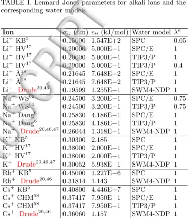
TABLE I. Lennard Jones parameters for alkali ions and the corresponding water models.
Ion σii(nm) ϵii(kJ/mol) Water model λa Li+ KB5 0.15000 1.547E+2 SPC 0.05 Li+ HV17 0.20000 5.000E−1 SPC/E 1 Li+ HV17 0.20000 5.000E−1 TIP3/P 1 Li+ HV17 0.20000 5.000E−1 TIP3/P 0.4 Li+ ˚A18 0.21645 7.648E−2 SPC/E 1 Li+ ˚A18 0.21645 7.648E−2 TIP3/P 1 Li+ Drude20,46 0.19599 1.255E−1 SWM4-NDP 1 Na+ WS62 0.24500 3.200E−1 SPC/E 0.75 Na+ WS62 0.24500 3.200E−1 TIP3/P 0.75 Na+ Dang6 0.25830 4.186E−1 SPC/E 1 Na+ Dang6 0.25830 4.186E−1 TIP3/P 1 Na+ Drude20,46,47 0.26044 1.318E−1 SWM4-NDP 1 K+ KB5 0.30300 2.185 SPC 1 K+ HV17 0.38000 2.000E−1 SPC/E 1 K+ HV17 0.38000 2.000E−1 TIP3/P 1 K+ Drude20,46,47 0.30052 5.938E−1 SWM4-NDP 1 Rb+ KB5 0.45000 1.227E−6 SPC 1 Rb+ Drude20,46 0.31814 1.143 SWM4-NDP 1 Cs+ KB5 0.40800 4.446E−7 SPC 1 Cs+ CHM58 0.37417 7.950E−1 SPC/E 1 Cs+ CHM58 0.37417 7.950E−1 TIP3/P 1 Cs+ Drude20,46 0.36060 1.157 SWM4-NDP 1
aScaling of the ion–water LJ interactions.
λ=1 if the interactions were not scaled.
TABLE II. Interatomic Lennard Jones parameters between the alkali ions (i) and water oxygens (j) after scaling.
Ion Water model λ σij(nm) ϵij(kJ/mol) Li+ KB5 SPC 0.05 0.2332785 0.501460 Li+ HV17 SPC/E 1 0.2582785 0.570172781 Li+ HV17 TIP3/P 1 0.22913925 0.564087759 Li+ HV17 TIP3/P 0.4 0.22913925 0.225635104 Na+ WS62 SPC/E 0.75 0.2807785 0.342104 Na+ WS62 TIP3/P 0.75 0.2800287 0.338452655
B. Analysis of the molecular dynamics simulations Radial distribution functions, (rdf, g(r)), were calcu-lated with the alkali ion as reference to the position of either of the oxygens in acetate (or water). The rdf were
normalized by the number of alkali ions, the volume of the bin width (0.002 nm), and the average particle den-sity of the acetate, so that the g(r) = 1 at infinity. The number of water molecules in first solvation shell was estimated from the average number of cation–water in-teractions within the ion-oxygen distances that are not larger than the first minimum of g(r).
Ion-acetate association constants (Ka [M−1]) were de-fined as:
Ka = [CH3COOM ]/([M+][CH3COO−]) (1)
where M = Li, Na, K, Rb or Cs. The association con-stants were calculated according to the equation15:
Ka= α/[(1− α)C] (2)
where α is the fraction of simulation time during which a contact ion pair (CIP) was present (i.e., when the metal to oxygen distance was smaller than the first rdf mini-mum, for numbers from respective simulation see Table S3), and C is the salt concentration. Free energies of complexation between ions and ligands were estimated as:
∆Ga =−RT lnKa. (3)
The activity coefficient (γ) was also calculated based on the time fraction spent in complex, α, and was hence simply defined as:
γ = 1− α (4)
The interaction energies, ∆Eint, between alkali ion and acetate were calculated from the simulations as a sum of the short-range LJ and Coulomb interaction energies between the components (ions and acetate molecules). The interaction energies were calculated for all simulation frames during which a contact ion pair (CIP) was present between an acetate and a cation. Similarly, ∆Eintvalues between alkali ion and water were calculated for Li+ and
Na+, with a criterion of four water ligands for Li+and six
water ligands for Na+. Since the larger ions (K+, Rb+
and Cs+) are softer and the first water shell was less distinct, the interaction energies could not be calculated in the same way for these ions.
C. Quantum chemistry
Interaction free energies (∆Gtot) were calculated as71: ∆Gtot= GP CMcomplex− (GP CMM+ + G
P CM
acetate) (5) where ∆Gtot is the free energy in solvent estimated by calculating the free energy of the solvated compound. The dielectric constant of the water was adjusted to the temperature, whereas vibrational effects are not consid-ered. ∆Gtot was decomposed into contributions from
electrostatics, exchange, repulsion, polarization, disper-sion and desolvation by Localized Molecular Orbital En-ergy Decomposition Analysis (LMOEDA)72as developed
for use with PCM (EDA-PCM)54,72. QM calculations
were carried out in GAMESS73. Water beyond the
first solvation shell (for hydrated complexes) or all wa-ter (for alkali ion-acetate complexes) were represented by PCM74. Energies were calculated with the MP2
method75. The def2-TZVPD76 basis set, used in
en-ergy calculations for all atoms, was downloaded from the EMSL basis set exchange database77,78. Effective core potentials (ECP) were applied for Rb (ECP-28) and Cs (ECP-46)79. Valence calculations for these ions were
performed with the def2-TZVPD basis set. The MP2 method and def2-TZVPD76basis set were used for
struc-ture optimization unless stated otherwise. Default sphere radii (as implemented in GAMESS80) were used for all atoms except Li+ for which no parameter was available
in the program. The sphere radius for Li+ was set to
0.59 nm following previous work4.
IV. RESULTS AND DISCUSSION A. Structural properties
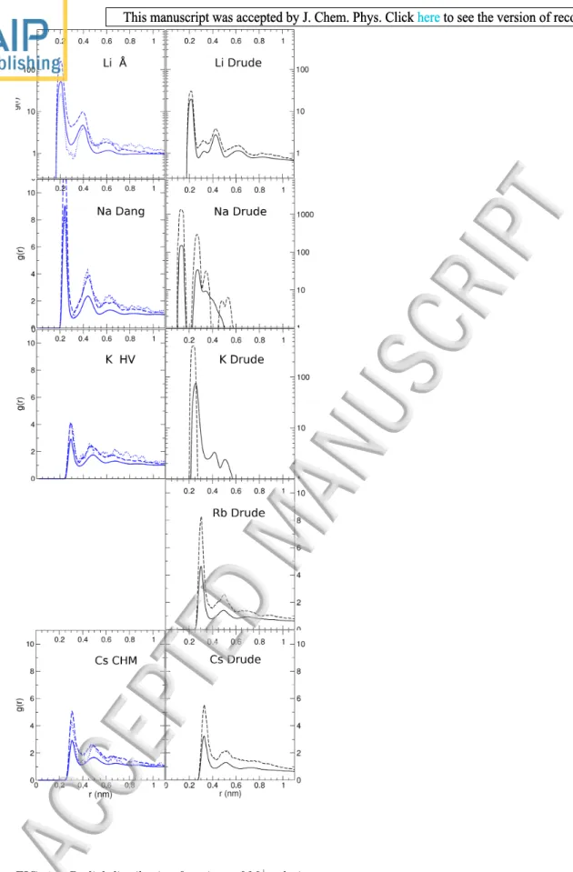
The radial distributions of acetate oxygens around al-kali ions simulated at different concentrations (0.03, 0.1, and 1 M) are summarized in Table III, and the rdf for one of the non-polarizable parameters (with the best matching log Ka-value) and the polarizable forcefields are shown in Figure 1. The first peak, r1, can be interpreted
as direct ion complexation or (closed sphere complex, or CIP). The second peak, r2, corresponds to a solvent
sep-arated ion pair interaction (solvent-sepsep-arated ion pair, SIP). Experimental values for distances between alkali ions and acetate were extracted from crystal structures of carboxylate-ion complexes deposited to the Cambridge Structural Database, CSD version 5.38 (Figure S1). A good agreement between the distances observed in the simulations and the crystallographic values (with differ-ences smaller than <0.01 nm) was observed with most of the FF combinations for ions and water. However, the use of the parameters developed by Hess and van-der-Vegt for the Li+ ion, with the scaling factor of 0.4 for the ionwater interaction resulted in SIP but not CIP for Li+–acetate interactions (in disagreement with the
crys-tal structures). Other dissimilarities involved the Drude-2013and KB-based parameters. The Drude polarizable parameters resulted in bond length between between Na+
and acetate that were too short. CIP distances were also smaller for Rb+ and Cs+ calculated with the
parame-ters derived based on Kirkwood-Buff theory for alkali-chlorides5, because the cations were too soft, i.e., the
LJ ϵ was rather small (which might have been necessary to obtain the right activities in alkali-chloride solutions). Further analysis was therefore not performed with those KB-based parameters. The rdf for Li-acetate simulated
with Drude polarizable forcefield showed a second peak at dCIP < d < dSIP. Examination of the simulations revealed a preference for a monodentate binding confor-mation for the Li-acetate complex studied with this force-field. This led to uneven distances between the small Li+
ion and the carboxylate oxygens, with the first peak (to the proximal oxygen) at 0.208 nm and the second peak (to the distal oxygen) at 0.325 nm.
The QM-optimized distances between alkali ion and the two acetate oxygen are given in Table III. QM dis-tances were 0.04 nm shorter than the reported crystallo-graphic measurements for Li+ and 0.01-0.02 nm shorter for the other cations. This ambiguity may stem from dif-ferent reasons, one of which is the choice of the atomic radii used in the PCM calculations. To examine the effect of the choice of radius for Li+, the ion-acetate complex was re-optimized after setting the ionic radius of Li+ to 0.70 nm. This resulted in ion-oxygen distances of 0.40 nm and 0.43 nm, which were 0.2 nm longer than the exper-imental value. For this reason, further calculations with rLi+ = 0.7 nm were not carried out, and the previously used radius (0.59 nm) was preferred. Other aspects that can contribute to the disagreement between the QM and experimental results are interactions with other atoms in the crystal, experimental inaccuracies, and the choice of solvent model, calculation method and basis set in QM calculations. Since the ions are not expected to maintain the minimal contact distance throughout the simulations, further efforts to examine this difference were not made. The number of water molecules in the first solvation shell and the peaks of ion–water rdf from the simulations are also reported in Table III. The use of the TIP3P water model generally resulted generally in a slightly larger number of water molecules in the rst solvation shell than for simulations with the SPC/E water model. For Li+, there were approximately ve water molecules in the
rst solvation shell with TIP3P rather than the expected number of four. Na+ ions were surrounded by 5-6 wa-ter molecules in the MD-simulations, and differences be-tween the non-polarizable simulations set ups were small. However, the use of the polarizable force field parame-ters for the Na+ resulted in strong association between
Na+and acetate during the simulations. Clusters of Na+ and acetate molecules were observed in the simulations, which indicated that the Na+ were only partly exposed
to the water molecules. Owing to the softer character and larger sizes of the Rb+and Cs+ions, the first
solva-tion shell of these ions was hard to define. The numbers of water molecules within the first solvation shells of Rb+ and Cs+ were estimated as 7.2 and 8-10, respectively.
B. QM interaction free energies and energy decomposition analysis
The calculated ion-acetate interaction free energies (∆Gtot) were−100 to −110 kJ/mol for the K+, Rb+and Cs+-acetate complexes, whereas the interactions were
more favorable for Na+-acetate (−130 kJ/mol) and Li+ -acetate (−150 kJ/mol). The contributions from polar-ization to the alkali ion-acetate were evaluated to ac-count for 23–56% of the total free energies of interac-tion based on PCM-EDA (Table IV). Although this contribution was very significant, it is much smaller in magnitude than ∆Gelec (which is large and negative) and ∆Gdesolv (which is large and positive). Polarization contributed more to the cation-acetate interactions than dispersion, and for Li+ and Na+ also more than QM
exchange. Interestingly, when examining ∆Gpol/∆Gtot the relative contribution of polarization is in the order Li+ > Cs+ > Rb+ > K+ > Na+. This is not in par of
the same calculation for the water complexes, where the order is Li+> Na+> K+∼ Rb+∼ Cs+. Overall, in the
case of Li+, polarization is more significant for
cation-water than for cation-acetate interactions, whereas for the other ions polarization is less significant (with respect to the overall interaction) when they are solvated.
C. Association constants
Reproducing the ion-carboxylate association constants is important for obtaining quantitative results from the simulations81. Overestimation of K
a results in over-binding, and in activity coefficients that are too low. Underestimation of Ka leads to ions that are too stable in water. In principle, reproducing the activity deriva-tives17 can yield parameters that reproduce the experi-mental values for the association constants irrespective of the salt concentration. Bjerrum estimated a critical distance for contact formation that depends on the ionic charge, solvent dielectric and temperature82, but not on
the specific ion. Here, the association constants were estimated from the simulations as KCIP, i.e., critical distances corresponded to the first minimum of the ion-oxygen rdf. The CIP-distances used for each calculation are presented in Table S3. Values of log KCIP are given in Table V and were compared to experimental log Ka for 0.1 M solutions. The association constants depend on the concentration, and should in principle be smaller for more concentrated solutions due to charge screening.
Examination of the KCIP values revealed that ion pair-ing between Li+ and acetate was too strong in almost all simulations, except for the scaled Li+ parameters (from Hess and van der Vegt) and the polarizable force-field were almost no CIP occurred. Overbinding was also observed in the simulations with the polarizable param-eters for Na+ and K+, which resulted in the formation
of Na-acetate salt clusters in the solutions. For Rb+and Cs+, K
CIP values calculated with the polarizable force-field were in good agreement with the experiment for 0.1 M solutions. The non-polarizable alkali ion parame-ters resulted in too negative log K values, i.e. complexes were disfavored. Some fixed atomic charge forcefields were off by as much as 0.7 log K units, whereas oth-ers were within 0.07-0.13 log K units, i.e., much closer to
the experimental values.
It is also possible to consider whether KSIP, i.e., set-ting up a cutoff that matches the second minimum in the cation-acetate rdf could be more appropriate as a theoretical match for the association constant. However, regardless of the ion and forcefield, calculated log KSIP values clearly overestimate log Ka (Table S3). Indeed, the generic cutoff suggested by Bjerrum for ions in water at T=298 K is 0.36 nm is within the range of distances for CIP (0.275-0.380 nm). The solvent-separated ion pair definition appears to be too loose for the purpose of cal-culating Ka from the simulations.
D. Energetics of the cation–acetate and cation–water interactions
The association constants can be used to calculate the free energies of complexation, which are given in Table V. These values can reveal whether and to which extent the differences between experimental and calculated associa-tion constants are meaningful compared to the thermal energy (2.48 kJ/mol). Indeed, most of forcefields param-eters used here resulted in reasonably accurate calcula-tions of the free energies of ion–acetate complexation at 0.1 M, and differences between the complexes simulated at the different concentrations were rather small (even for Li+, where ∆G
exp= 0.25 kJ/mol, calculated from Ka). A single exception was the value obtained with the scaled non-polarizable Li+ parameters (HV), ∆G= 14 kJ/mol.
For Na+, the WS parameter set underestimates the bind-ing free energies by some 4 kJ/mol. A common test for the accuracy of ion forcefields is the ability to reproduce the hydration free energies, which is in itself not a triv-ial experimental value to compare with20. It is possible
to get the cation hydration free energies right but still over- or underestimate the complexation energies, which depends on the cation–acetate and acetate–water inter-actions as well. The interaction energies, ∆Eint for the cation–acetate and cation–water-shell can be calculated directly from the simulations if a non-polarizable force-field is used and the solvation shell is defined. Those val-ues were given (when possible) in Table V. This analysis revealed that the main difference between the WS and Dang parameter sets for Na+was due to the interactions
between the ions and water molecules.
E. Activity coefficients
The activity coefficients, γ, were estimated experimen-tally to be ∼0.8 for all alkali–acetate salts in 0.1 M so-lutions83. In 1 M solutions, the difference between Li+,
Na+ and the larger alkali ions was more eminent
(Ta-ble V). The decrease of the value of γ was most apparent for Li–acetate solutions (∆γ =−0.11 when a solution is concentrated from 0.1 to 1 M), smaller for Na–acetate (∆γ =−0.04), and not apparent in solutions containing
the larger alkali cations. The activity coefficients were calculated from the simulations in order to examine how well the different forcefields reproduced the experimental values (Table V). For Li+, the non-polarizable parameter
set from ˚Aqvist simulated with SPC/E water resulted in activity coefficients that were in par with the experimen-tal values at 0.1 M, whereas the HV parameter set and the polarizable force field parameters overestimated γ at the same concentration. The situation was different with 1 M solutions, where the activity coefficient was underes-timated by all forcefields, with the polarizable parameter set leading to the best agreement with the experiment. For Na+, calculations of γ from simulations with the
pa-rameter set from Dang, but not WS, resulted in a value very similar to the experiment for 1 M sodium acetate. One explanation for the higher γ obtained from simula-tions of Na–acetate with the parameters from Weeras-inghe and Smith can be that the Na+–water interaction
energy was too favorable, so that the Na+ion had a
ten-dency to stay solvated.
The calculated activity coefficients for 0.1 M solutions of Na, K, Rb and Cs–acetate were lower than the values estimated from experiments, regardless of the parameter set, whereas better agreement between simulation and experiment was observed in 1 M solutions. In 0.1 M electrolyte solutions, the average distance between two oppositely charged ions is much larger than the cutoff (the density of each ion is 0.06 ions/nm3, and their aver-age distance would thus be 2.59 nm if they are randomly dispersed). In 1 M solutions, chance encounters within 1.0 nm are much more common (the average distance between the ions would be 1.22 nm if they are randomly dispersed). Of note, the diffusion coefficients of the ions are in par with the experiment (Table S4), which indi-cates that the dynamics are realistic.
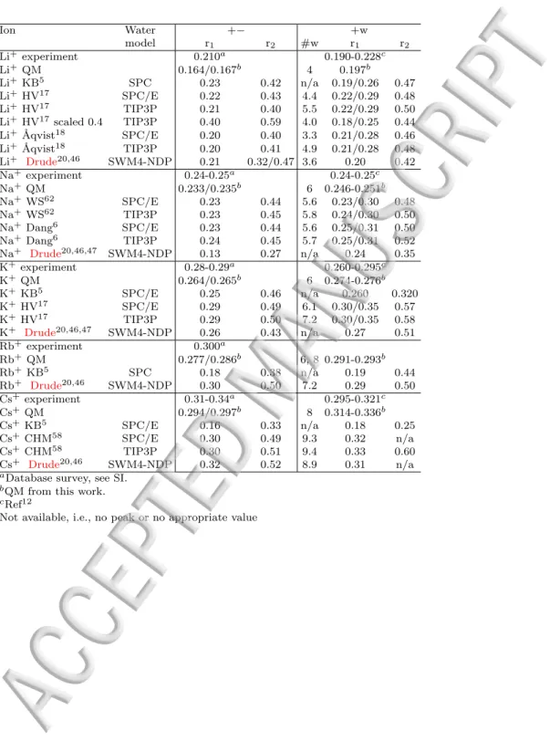
TABLE III. Radial distribution functions (rdf) calculated from MD simulations for cation–acetate (+−) and metal cation–water oxygen (+w) (values are calculated from 1 M concentration simulations). r1 and r2 is the separation dis-tances in nm for the first and second peak maximum. #w is the average number of water molecules in the first solvation shell calculated from simulations carried out with the lowest concentration of ions, i.e. 0.03 M or 0.1 M.
Ion Water +− +w model r1 r2 #w r1 r2 Li+ experiment 0.210a 0.190-0.228c Li+ QM 0.164/0.167b 4 0.197b Li+ KB5 SPC 0.23 0.42 n/a 0.19/0.26 0.47 Li+ HV17 SPC/E 0.22 0.43 4.4 0.22/0.29 0.48 Li+ HV17 TIP3P 0.21 0.40 5.5 0.22/0.29 0.50 Li+ HV17scaled 0.4 TIP3P 0.40 0.59 4.0 0.18/0.25 0.44 Li+ ˚Aqvist18 SPC/E 0.20 0.40 3.3 0.21/0.28 0.46 Li+ ˚Aqvist18 TIP3P 0.20 0.41 4.9 0.21/0.28 0.48 Li+ Drude20,46 SWM4-NDP 0.21 0.32/0.47 3.6 0.20 0.42 Na+experiment 0.24-0.25a 0.24-0.25c Na+QM 0.233/0.235b 6 0.246-0.251b Na+WS62 SPC/E 0.23 0.44 5.6 0.23/0.30 0.48 Na+WS62 TIP3P 0.23 0.45 5.8 0.24/0.30 0.50 Na+Dang6 SPC/E 0.23 0.44 5.6 0.25/0.31 0.50 Na+Dang6 TIP3P 0.24 0.45 5.7 0.25/0.31 0.52 Na+ Drude20,46,47 SWM4-NDP 0.13 0.27 n/a 0.24 0.35 K+experiment 0.28-0.29a 0.260-0.295c K+QM 0.264/0.265b 6 0.274-0.276b K+KB5 SPC/E 0.25 0.46 n/a 0.260 0.320 K+HV17 SPC/E 0.29 0.49 6.1 0.30/0.35 0.57 K+HV17 TIP3P 0.29 0.50 7.2 0.30/0.35 0.58 K+ Drude20,46,47 SWM4-NDP 0.26 0.43 n/a 0.27 0.51 Rb+ experiment 0.300a Rb+ QM 0.277/0.286b 6, 8 0.291-0.293b Rb+ KB5 SPC 0.18 0.38 n/a 0.19 0.44 Rb+ Drude20,46 SWM4-NDP 0.30 0.50 7.2 0.29 0.50 Cs+ experiment 0.31-0.34a 0.295-0.321c Cs+ QM 0.294/0.297b 8 0.314-0.336b Cs+ KB5 SPC/E 0.16 0.33 n/a 0.18 0.25 Cs+ CHM58 SPC/E 0.30 0.49 9.3 0.32 n/a Cs+ CHM58 TIP3P 0.30 0.51 9.4 0.33 0.60 Cs+ Drude20,46 SWM4-NDP 0.32 0.52 8.9 0.31 n/a
aDatabase survey, see SI. bQM from this work. cRef12
FIG. 1. Radial distribution functions of M+ relative to ac-etate oxygen atoms simulated in 0.03 M (dotted lines), 0.1 M (dashed lines) and 1 M (solid lines) concentrations. Non-polarizable forcefields (simulations with SPC/E water) are shown in the left panels and polarizable forcefields in the pan-els to the right. The curves were smoothed by averaging the measurements over 20 steps to remove spurious jumps. The forcefield parameter sets are given in Table I.
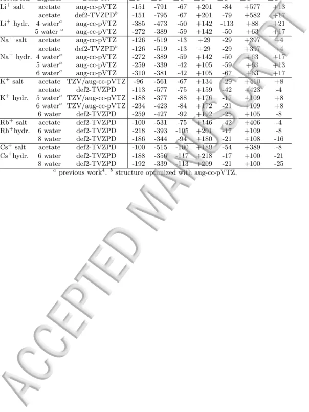
TABLE IV. Free energies of interaction (∆Gint) between al-kali ion–acetate and alal-kali ion–water in PCM, decomposed by EDA-PCM54 into contributions from electrostatics (∆Gele), exchange (∆Gex), repulsion (∆Grep), polarization (∆Gpol), desolvation (∆Gdesol) and dispersion (∆Gdisp). The values were obtained with MP2 and are given in kJ/mol.
Metal ion Ligands Basis set ∆Gtot ∆Gele ∆Gex ∆Grep ∆Gpol ∆Gdesol ∆Gdisp Li+ salt acetate aug-cc-pVTZ -151 -791 -67 +201 -84 +577 +13
acetate def2-TVZPDb -151 -795 -67 +201 -79 +582 +17 Li+ hydr. 4 watera aug-cc-pVTZ -385 -473 -50 +142 -113 +88 +21 5 watera aug-cc-pVTZ -272 -389 -59 +142 -50 +63 +17 Na+ salt acetate aug-cc-pVTZ -126 -519 -13 +29 -29 +397 +4
acetate def2-TVZPDb -126 -519 -13 +29 -29 +397 +4 Na+ hydr. 4 watera aug-cc-pVTZ -272 -389 -59 +142 -50 +63 +17
5 watera aug-cc-pVTZ -259 -339 -42 +105 -59 +63 +13 6 watera aug-cc-pVTZ -310 -381 -42 +105 -67 +63 +17 K+salt acetate TZV/aug-cc-pVTZ -96 -561 -67 +134 -29 +410 +8
acetate def2-TVZPD -113 -577 -75 +159 -42 +423 -4 K+hydr. 5 watera TZV/aug-cc-pVTZ -188 -377 -88 +176 -17 +109 +8
6 watera TZV/aug-cc-pVTZ -234 -423 -84 +172 -21 +109 +8 6 water def2-TVZPD -259 -427 -92 +192 -25 +105 -8 Rb+ salt acetate def2-TVZPD -100 -531 -75 +146 -42 +406 -4 Rb+hydr. 6 water def2-TVZPD -218 -393 -105 +201 -17 +109 -8 8 water def2-TVZPD -186 -344 -94 +180 -21 +108 -16 Cs+ salt acetate def2-TVZPD -100 -515 -100 +180 -54 +389 -8 Cs+hydr. 6 water def2-TVZPD -188 -356 -117 +218 -17 +100 -21 8 water def2-TVZPD -192 -339 -113 +209 -21 +100 -25
TABLE V. Equilibrium constants (experimental log Ka and calculated log KCIP), free energies of complexation (∆G), activity coefficients (γ) and interaction energies (∆E) for the alkali ion–acetate and the alkali ion–water interactions in solu-tions at 298 K for different concentrasolu-tions. Critical radii used in the calculations of log K, ∆G and activity calculations are based on CIP distances (Table S3). For the non-polarizable forcefields, results are averages (standard deviations) of five simulations (100 ns each). The polarizable forcefield parame-ters were calculated from five 10 ns simulations.
Ion Water Concentration log K ∆G (kJ/mol) γ ∆Eintion- ∆Eint
ion-model (M) MD exp.84 MD exp. MD exp. acetate (kJ/mol) water (kJ/mol)
Li+ HV17 SPC/E 0.03 +0.17(13) −1.05 0.96 −178 −240 0.1 +0.00(3) −0.11 0 +0.25 0.91 0.79 1 −0.09(3) 0 0.55 0.69 Li+ HV17 TIP3P 0.03 +0.28(20) −1.90 0.94 −218 −473a 0.1 −0.04(20) −0.11 0 +0.25 0.91 0.79 1 +0.32(4) −1.90 0.32 0.69 Li+ HV17 TIP3P 0.03 −2.00(0) +11.0 1.00 n/a −629 scaled 0.4 0.1 −2.50(4) −0.11 +14.0 +0.25 1.00 0.79 1 +0.60(4) −3.80 0.18 0.69 Li+ ˚A18 SPC/E 0.03 +0.47(45) −3.40 0.90 −206 −413 0.1 +0.33(11) −0.11 −2.30 +0.25 0.80 0.79 1 +0.33(2) −1.85 0.32 0.69 Li+ ˚A18 TIP3P 0.03 +0.57(44) −4.00 0.87 −232 −495 0.1 +0.70(13) −0.11 −4.10 +0.25 0.66 0.79 1 +0.33(2) −1.85 0.32 0.69 Li+ Drude20,46 SWM4-NDP 0.1 −2.00(100) −0.11 +5.0 +0.25 0.99 0.79 1 −0.22(10) +1.2 0.62 0.69 Na+WS62 SPC/E 0.03 −0.93(30) +4.80 1.00 −134 −340 0.1 −0.96(11) −0.26 +5.40 +0.65 0.99 0.79 1 −1.07(2) +6.10 0.92 0.75 Na+WS62 TIP3P 0.03 −0.96(46) +4.55 1.00 −178 −424 0.1 −0.91(14) −0.26 +5.10 +0.65 0.99 0.79 1 −0.93(1) +5.30 0.90 0.75 Na+Dang6 SPC/E 0.03 −0.29(14) +1.60 0.98 −124 −285 0.1 −0.39(8) −0.26 +2.20 +0.65 0.96 0.79 1 −0.47(1) +2.65 0.75 0.75 Na+Dang6 TIP3P 0.03 −0.41(26) +1.90 0.99 −188 −359 0.1 −0.32(4) −0.26 +1.85 +0.65 0.96 0.79 1 −0.32(1) +1.85 0.68 0.75 Na+ Drude20,46,47 SWM4-NDP 0.1 −0.26 +0.65 0.79 1 Cluster formation 0.75 K+HV17 SPC/E 0.03 −0.41(6) +2.40 0.99 −60 0.1 −0.52(3) −0.41 +2.95 +1.00 0.97 0.79 1 −0.66(0) +3.75 0.82 0.78 K+HV17 TIP3P 0.03 −0.74(15) +4.05 0.99 −89 0.1 −0.68(2) −0.41 +3.90 +1.00 0.98 0.79 1 −0.73(1) +4.20 0.84 0.78 K+ Drude20,46,47 SWM4-NDP 0.1 +1.30(23) −0.41 −7.5 +1.00 0.36 0.79 1 +1.20(11) −7.0 0.06 0.78 Rb+ Drude20,46 SWM4-NDP 0.1 −0.32(13) −0.35 +1.70 +0.85 0.95 0.78 1 −0.44(2) +2.50 0.74 0.79 Cs+ CHM58 SPC/E 0.03 −0.40(11) +2.15 0.95 −53 0.1 −0.38(2) −0.31 +2.15 +0.75 0.96 0.79 1 −0.55(6) +3.10 0.78 0.80 Cs+ CHM58 TIP3P 0.03 −0.56(10) +3.15 0.99 −79 0.1 −0.58(2) −0.31 +3.30 +0.75 0.98 0.79 1 −0.63(1) +3.60 0.81 0.80 Cs+ Drude20,46 SWM4-NDP 0.1 −0.29(7) −0.31 +1.65 +0.75 0.95 0.79 1 −0.44(1) +2.55 0.74 0.80
V. CONCLUSIONS
Extensive simulations of alkali–acetate solutions were performed with different polarizable and non-polarizable forcefield parameters. Observables were calculated from the simulations and compared to experimental measure-ments that are relevant to simulations of proteins in so-lutions. QM EDA calculations were performed in order to estimate the contributions of polarizability and non-classical contributions to the interaction energies between the ions and acetates. Some of the parameters did not reproduce the correct rdf structures for the solutions. For all alkali ions except Li+, good agreement between
calculated and experimentally observed activity coeffi-cients was obtained in 1 M concentrated solutions by at least one of the tested parameter sets. Activity co-efficients were overestimated for the non-Li+ ions when simulated in 0.1 M solutions. On the other hand, cal-culated complexation free energies were in most cases within few kJ/mol or less of the experimental values, and the simulations reproduced the higher propensity to ob-serve ion–acetate complexes in lower concentrations in density-normalized rdf. EDA calculations revealed that although the contribution of polarization with respect to the overall interaction energy between the ions and the acetates was significant, it was much smaller than the electrostatic contribution. Polarization, however, was shown to be important for Li+–water interactions. Differ-ences between the non-polarizable forcefield parameters for Na+ appeared to be due to the interactions between
the cations and the water, and point out that further tuning the ion–water interactions may be important to achieve better agreement with the experiment when in-teractions with carboxylates are considered.
Overestimation of the activity coefficients in 0.1 M so-lutions of non-Li+ alkali ions was systematic, and stood
in contrast to the agreement between simulation and ex-periment in 1 M solutions. Since none of the water mod-els that were employed in the simulations overestimated the dielectric constant of the water, it is not likely that the screening of the charge-charge interactions was the source of this discrepancy. Instead, it may well be that the simulation protocol, which uses finite interaction cut-off was the source of this artifact. It can be expected that this would be less pronounced on the surface of proteins, when the acetates are more static and the Coulomb cage extends to a larger volume3,15.
Simulations of Li+–acetate solutions did not achieve
an overall good agreement with the experiment. The polarizable parameters reproduced all observables well when the solution concentration was 1 M, but when it was smaller. The ˚Aqvist parameters with SPC/E water yielded activity coefficients that were close to the exper-imental values for 0.1 M solutions, but were too low for 1 M solutions, whereas calculations of the activity coeffi-cient were closer to the experimental value when carried out with the HV parameter set in a 1 M Li–acetate so-lution. Since the simulation protocol was similar for the
different alkali ions, agreement with the experiment at 0.1 M may be due to cancellation of errors (the force-fields overestimated the anion-cation interactions, which compensated for the opposite effect introduced by the Coulomb cutoff). EDA calculations revealed that the contributions of the exchange interaction to the overall free energy of interaction between Li+ and water or ac-etate was not higher than for other ions, whereas polar-ization was important for Li+–water interactions. Thus,
developing forcefield parameters that could represent the interactions between Li+, carboxylates and water more realistically should be achievable, but may require a po-larizable model.
VI. SUPPLEMENTARY MATERIAL
See supplementary material for CGenFF acetate pa-rameters and papa-rameters for all ions for the polarizable force field, critical radius values and equilibrium con-stants for SIP, diffusion concon-stants and distribution of crystallographic distances between carboxylate oxygens and alkali cations.
ACKNOWLEDGMENTS
Some of the simulations were performed on resources provided by the Swedish National Infrastructure for Computing (SNIC) at the center for scientific and tech-nical computing at Lund University (LUNARC), project SNIC 2016/1-518. This study was supported in part by the Swedish Research Council, grant number VR 2014-04406. JZS thanks the Brazilian National Council for Scientific and Technological Development for a scholar-ship (CNPq-305626/2013-2).
1R. Friedman, E. Nachliel, and M. Gutman, Bioch. Bioph. Acta.
1710, 67 (2005).
2M. Gutman, E. Nachliel, and R. Friedman, Photochem.
Photo-biol. Sci. 5, 531 (2006).
3R. Friedman, J. Phys. Chem. B 115, 9213 (2011).
4O. Becconi, E. Ahlstrand, A. Salis, and R. Friedman, Israel J.
Chem. 57, 403 (2017).
5B. Klasczyk and V. Knecht, J. Chem. Phys. 132, 024109 (2010). 6L. X. Dang, J. Am. Chem. Soc. 117, 6954 (1995).
7P. Jungwirth and D. J. Tobias, Chem. Rev. 106, 1259 (2006). 8E. F. Aziz, N. Ottosson, S. Eisebitt, W. Eberhardt, B.
Jagoda-Cwiklik, R. Vcha, P. Jungwirth, and B. Winter, J. Phys. Chem. B 112, 12567 (2008).
9R. Friedman, J. Chem. Edu. 90, 1018 (2013).
10T. X. Dang and E. W. McCleskey, J. Gen. Physiol. 111, 185
(1998).
11E. Project, R. Friedman, E. Nachliel, and M. Gutman, Biophys.
J. 90, 3842 (2006).
12H. Ohtaki and T. Radnai, Chem. Rev. 93, 1157 (1993). 13H. I. Okur, J. Kherb, and P. S. Cremer, J. Am. Chem. Soc. 135,
5062 (2013).
14R. Friedman, E. Nachliel, and M. Gutman, J. Biol. Phys. 31,
433 (2005).
15R. Friedman, E. Nachliel, and M. Gutman, Biophys. J. 89, 768
16E. Project, E. Nachliel, and M. Gutman, PLoS One 6, 21364983
(2011).
17B. Hess and N. F. van der Vegt, Proc. Natl. Acad. Sci. U.S.A.
106, 13296 (2009).
18J. ˚Aqvist, J. Chem. Phys. 94, 8021 (1990).
19B. Roux and M. Karplus, J. Phys. Chem. 95, 4856 (1991). 20H. Yu, T. W. Whitfield, E. Harder, G. Lamoureux, I. Vorobyov,
V. M. Anisimov, A. D. MacKerell, and B. Roux, J. Chem. The-ory Comput. 6, 774 (2010).
21L. X. Dang and T.-M. Chang, J. Chem. Phys. 106, 8149 (1997). 22D. Jiao, C. King, A. Grossfield, T. A. Darden, and P. Ren, J.
Phys. Chem. B 110, 18553 (2006).
23N. Gresh, G. A. Cisneros, T. A. Darden, and J.-P. Piquemal, J.
Chem. Theory Comput. 3, 1960 (2007).
24B. de Courcy, J.-P. Dognon, C. Clavagu´era, N. Gresh, and J.-P.
Piquemal, Int. J. Quant. Chem. 111, 1213 (2011).
25M. Soniat and S. W. Rick, J. Chem. Phys. 140, 184703 (2014). 26T. Dudev, M. Devereux, M. Meuwly, C. Lim, J. P. Piquemal,
and N. Gresh, J Comput Chem 36, 285 (2015).
27G. E. Marlow and B. M. Pettitt, Biopolymers 60, 134 (2001). 28L. Vrbka, P. Jungwirth, P. Bauduin, D. Touraud, and W. Kunz,
J. Phys. Chem. B 110, 7036 (2006).
29S. J. Lee, Y. Song, and N. A. Baker, Biophys. J. 94, 3565 (2008). 30J. Heyda, J. Pokorn´a, L. Vrbka, R. V´acha, B. Jagoda-Cwiklik,
J. Konvalinka, P. Jungwirth, and J. Vondr´asek, Phys Chem Chem Phys 11, 7599 (2009).
31D. Horinek, S. I. Mamatkulov, and R. R. Netz, J. Chem. Phys.
130, 124507 (2009).
32S. Pokorna, P. Jurkiewicz, L. Cwiklik, M. Vazdar, and M. Hof,
Faraday Discuss. 160, 341 (2013).
33P. Ganguly, T. Hajari, and N. F. A. van der Vegt, J. Phys.
Chem. B 118, 5331 (2014).
34F. R. Beierlein, T. Clark, B. Braunschweig, K. Engelhardt,
L. Glas, and W. Peukert, J Phys Chem B 119, 5505 (2015).
35L. Pineda De Castro, M. Dopson, and R. Friedman, J. Phys.
Chem. B 120, 10628 (2016).
36G. Lamoureux, A. D. M. Jr., and B. Roux, J. Chem. Phys. 119,
5185 (2003), http://dx.doi.org/10.1063/1.1598191.
37B. R. Brooks, R. E. Bruccoleri, B. D. Olafson, D. J. States,
S. Swaminathan, and M. Karplus, J. Comp. Chem. 4, 187 (1983).
38B. R. Brooks, C. L. Brooks, A. D. MacKerell, L. Nilsson,
B. Roux, Y. Won, G. Archontis, C. Bartels, S. Boresch, A. Caflisch, L. Caves, Q. Cui, A. Dinner, S. Fischer, J. Gao, M. Hodoscek, K. Kuczera, T. Lazaridis, J. Ma, E. Paci, R. W. Pastor, C. B. Post, M. Schaefer, B. Tidor, R. W. Venable, H. L. Woodcock, X. Wu, and M. Karplus, J. Comp. Chem. 30, 1545 (2009).
39J. A. Lemkul, B. Roux, D. van der Spoel, and A. D. MacKerell,
J. Comput. Chem. 36, 1473 (2015).
40H. J. C. Berendsen, D. van der Spoel, and R. Vandrunen,
Com-put. Phys. Commun. 91, 43 (1995).
41D. van der Spoel, E. Lindahl, B. Hess, G. Groenhof, A. E. Mark,
and H. J. C. Berendsen, J. Comput. Chem. 26, 1701 (2005).
42M. J. Abraham, T. Murtola, R. Schulz, S. Pll, J. C. Smith,
B. Hess, and E. Lindahl, SoftwareX 12, 19 (2015).
43W. Jiang, D. J. Hardy, J. C. Phillips, A. D. MacKerell,
K. Schulten, and B. Roux, J. Phys. Chem. Lett. 2, 87 (2011), http://dx.doi.org/10.1021/jz101461d.
44J. C. Phillips, R. Braun, W. Wang, J. Gumbart, E. Tajkhorshid,
E. Villa, C. Chipot, R. D. Skeel, L. Kal´e, and K. Schulten, J Comput Chem 26, 1781 (2005).
45H. V. Annapureddy and L. X. Dang, J Phys Chem B 116, 7492
(2012).
46Y. Luo, W. Jiang, H. Yu, A. D. MacKerell, and B. Roux, Faraday
Discuss. 160, 135 (2013).
47H. Li, V. Ngo, M. C. Da Silva, D. R. Salahub, K. Callahan,
B. Roux, and S. Y. Noskov, J. Phys. Chem. B 119, 9401 (2015).
48S. B. Rempe, L. R. Pratt, G. Hummer, J. D. Kress, R. L. Martin,
and A. Redondo, J. Am. Chem. Soc. 122, 966 (2000).
49S. B. Rempe and L. R. Pratt, Fluid Phase Equilibria 183-184,
121 (2001).
50K. Leung, S. B. Rempe, and O. A. von Lilienfeld, J. Chem. Phys.
130, 204507 (2009).
51C. N. Rowley and B. Roux, J. Chem. Theory. Comput. 8, 3526
(2012).
52A. Y. Mehandzhiyski, E. Riccardi, T. S. van Erp, T. T. Trinh,
and B. A. Grimes, J Phys Chem B 119, 10710 (2015).
53J.-P. Piquemal, L. Perera, G. A. Cisneros, P. Ren, L. G. Pedersen,
and T. A. Darden, J. Chem. Phys. 125, 054511 (2006).
54P. Su, H. Liu, and W. Wu, J. Chem. Phys. 137, 034111 (2012). 55K. Vanommeslaeghe, E. Hatcher, C. Acharya, S. Kundu,
S. Zhong, J. Shim, E. Darian, O. Guvench, P. Lopes, I. Vorobyov, and A. D. Mackerell, J. Comput. Chem. 31, 671 (2010).
56A. D. MacKerell, D. Bashford, M. Bellott, R. L. Dunbrack,
J. D. Evanseck, M. J. Field, S. Fischer, J. Gao, H. Guo, S. Ha, D. Joseph-McCarthy, L. Kuchnir, K. Kuczera, F. T. K. Lau, C. Mattos, S. Michnick, T. Ngo, D. T. Nguyen, B. Prodhom, W. E. Reiher, B. Roux, M. Schlenkrich, J. C. Smith, R. Stote, J. Straub, M. Watanabe, J. Wiorkiewicz-Kuczera, D. Yin, and M. Karplus, J. Phys. Chem. B 102, 3586 (1998).
57A. D. Mackerell, M. Feig, and C. L. Brooks, J. Comput. Chem.
25, 1400 (2004).
58P. Bjelkmar, P. Larsson, M. A. Cuendet, B. Hess, and E. Lindahl,
J. Chem. Theory Comput. 6, 459 (2010).
59H. J. C. Berendsen, J. R. Grigera, and T. Straatsma, J. Phys.
Chem. 91, 6269 (1987).
60H. J. C. Berendsen, J. P. M. Postma, W. F. van Gunsteren, and
J. Hermans, Interaction models for water in relation to protein
hydration., Intermolecular Forces. (D. Reidel Publishing
Com-pany Dordrecht, 1981).
61E. Ahlstrand, D. Sp˚angberg, K. Hermansson, and R. Friedman,
Int. J. Quant. Chem. 113, 2554 (2013).
62S. Weerasinghe and P. E. Smith, J Chem Phys 119, 11342 (2003). 63B. Hess, H. Bekker, H. J. C. Berendsen, and J. G. E. M. Fraaije,
J. Comp. Chem. 18, 1463 (1997).
64S. Miyamoto and P. A. Kollman, J. Comp. Chem. 13, 952 (1992). 65G. Bussi, D. Donadio, and M. Parrinello, J. Chem. Phys. 126,
014101 (2007).
66M. Parrinello and A. Rahman, J. Appl. Phys. 52, 7182 (1981). 67T. Darden, D. York, and L. Pedersen, J. Chem. Phys. 98, 10089
(1993).
68S. Jo, T. Kim, V. G. Iyer, and W. Im, J. Comput. Chem. 29,
1859 (2008).
69P. E. M. Lopes, J. Huang, J. Shim, Y. Luo, H. Li, B. Roux, and
A. D. MacKerell, J. Chem. Theory Comput. 9, 5430 (2013).
70G. Lamoureux, E. Harder, I. V. Vorobyov, B. Roux, and A. D. M.
Jr., Chem. Phys. Lett. 418, 245 (2006).
71E. Ahlstrand, K. Hermansson, and R. Friedman, J. Phys. Chem.
A 121, 2643 (2017).
72S. Peifeng and L. Hui, J. Chem. Phys. 131, 014102 (2009). 73M. W. Schmidt, K. K. Baldridge, J. A. Boatz, S. Elbert, M.
Gor-don, J. H. Jensen, S. Koseki, N. Matsunaga, K. A. Nguyen, S. Su, T. L. Windus, M. Dupuis, and J. A. Montgomery, J. Comput. Chem. 14, 1347 (1993).
74H. Li and J. H. Jensen, J. Comput. Chem. 25, 1449 (2004). 75C. Møller and M. Plesset, Phys. Rev. 46, 0618 (1934).
76D. Rappoport and F. Furche, J. Chem. Phys. 133, 134105 (2010). 77D. Feller, J. Comput. Chem. 17, 1571 (1996).
78K. L. Schuchardt, B. T. Didier, T. Elsethagen, L. Sun, V.
Gu-rumoorthi, J. Chase, J. Li, and T. L. Windus, J. Chem. Info. Model. 47, 1045 (2007).
79T. Leininger, A. Nicklass, W. Kuchle, H. Stoll, M. Dolg, and
A. Bergner, Chem. Phys. Lett. 255, 274 (1996).
80A. Bondi, J. Phys. Chem. 68, 441 (1964).
81E. Project, E. Nachliel, and M. Gutman, J Comput Chem 29,
1163 (2008).
82N. Bjerrum, Danske Vidensk Selskab 7, 1 (1926).
83R. A. Robinson and R. H. Stokes, Electrolyte solutions
84A. E. Martell and R. M. Smith, Critical stability constants, Vol. 1