Distributed Computing in Peer-to-peer Networks

Distributed Computing in Peer-to-peer

Networks

Emir Ahmetspahi´

c

LITH-IDA-EX–04/095–SE

Link¨opings Universitet

Institutionen f¨or datavetenskap

Final Thesis

Distributed Computing in Peer-to-peer

Networks

by

Emir Ahmetspahi´

c

LITH-IDA-EX–04/095–SE

2004-09-27

Supervisor: Niclas Andersson Examiner: Nahid Shahmehri

Avdelning, Institution Division, Department Institutionen för datavetenskap 581 83 LINKÖPING Datum Date 2004-09-27 Språk

Language RapporttypReport category ISBN Svenska/Swedish

X Engelska/English X ExamensarbeteLicentiatavhandling ISRN LITH-IDA-EX--04/095--SE C-uppsats

D-uppsats Serietitel och serienummer_{Title of series, numbering} ISSN Övrig rapport

____

URL för elektronisk version

http://www.ep.liu.se/exjobb/ida/2004/dd-d/095/

Titel

Title Distributed Computing in Peer-to-peer Networks

Författare

Author Emir Ahmetspahic

Sammanfattning

Abstract

Concepts like peer-to-peer networks and distributed computing are not new. They have been available in different forms for a long time. This thesis examines the possibility of merging these concepts. The assumption is that non-centralized peer-to-peer networks can be used for effective sharing of computing resources. While most peer-to-peer systems today concentrate on sharing of data in various forms, this thesis concentrates on sharing of clock cycles instead of files.

Nyckelord

Keyword

Abstract

Concepts like peer-to-peer networks and distributed computing are not new. They have been available in different forms for a long time. This thesis examines the possibility of merging these concepts. The assumption is that non-centralized peer-to-peer networks can be used for effective sharing of computing resources. While most peer-to-peer systems today concentrate on sharing of data in various forms, this thesis concentrates on sharing of clock cycles instead of files.

Contents

Preface 11

About report . . . 11

About the author . . . 11

About the supervisors . . . 11

Acknowledgements . . . 12

1 Introduction 13 1.1 Goals and Requirements . . . 13

1.2 Lack of Centralized Services . . . 14

1.3 Full Security Model . . . 14

1.4 Full Brokering Capabilities . . . 15

1.5 Limitations . . . 15

2 Concepts and Related Works 17 2.1 Distributed Supercomputing . . . 17

2.1.1 Related Works . . . 19

2.2 Peer-to-peer Networks . . . 21

2.2.1 Service Architectures . . . 22

2.2.2 Internet History Through Different Architectures . . . 24

2.2.3 Related Works . . . 25 3 Theory 31 3.1 Communication . . . 32 3.1.1 Finding Hosts . . . 34 3.1.2 Establishing Connection . . . 34 3.1.3 Permanent Connections . . . 35 3.1.4 Temporary Connections . . . 36

3.1.6 Maintaining Connection . . . 37

3.1.7 Ending Connection . . . 38

3.1.8 Sending Request for Offers . . . 39

3.1.9 Examples . . . 39

3.2 Brokering . . . 44

3.2.1 Job and Machine Descriptions . . . 44

3.2.2 Rules . . . 45

3.3 Security . . . 55

3.3.1 Different Cryptographic Concepts . . . 56

3.3.2 Threats and Suggested Solutions . . . 60

4 Implementation 65 4.1 Example . . . 67

5 Evaluation 69

6 Discussion and Future Work 73

A XML Schema 77

Preface

This chapter contains background information about this master thesis. Also there is contact information for the author and supervisors of this thesis.

About report

During the fall of 2002 I had several ideas about what to do for my master thesis. All these ideas had one thing in common - distributed computing. In November 2002, I contacted Niclas Andersson at National Supercomputing Centre (NSC) in Link¨oping. After meeting with Niclas Andersson and Leif Nixon my ideas were somewhat modified. In late October 2003 I started working on my master thesis. The result of this work is presented in this report.

About the author

The author of this report is Emir Ahmetspahi´c. I am currently completing my final year as a student in the Master of Science Programme in Communication and Transportation Engineering at Link¨oping University. I can be reached at the following e-mail address: emiah182@student.liu.se

About the supervisors

The supervisor of this master thesis was Niclas Andersson. He currently works as a parallel computing expert at the National Supercomputing Centre (NSC) in Link¨oping, Sweden. Niclas can be reached at the following e-mail address: nican@nsc.liu.se

Formal examinator of this thesis was Nahid Shahmehri. She is professor in computer science at the Department of Computer and Information Science (IDA), Link¨oping University in Link¨oping, Sweden. She is currently also

director of the Laboratory for Intelligent Information (IISLAB). She can be reached at the following e-mail address: nahsh@ida.liu.se

Acknowledgements

First and foremost I would like to thank Niclas Andersson. He has been extremely helpful and always took the time to point out errors and explain different concepts I did not understand previously. Also I would like to thank Leif Nixon who corrected countless mistakes in English grammar that were present in the first draft of this report. He also offered many useful programming advices. Finally, I wish to thank all other personnel at the National Computing Centre in Link¨oping that made my stay there a pleasant one.

Chapter 1

Introduction

As it can be noticed by the title of this report, this study concerns itself with the distribution of computing power in peer-to-peer networks. This chapter presents the goal of the thesis and requirements that need to be satisfied so that this master thesis can be considered successful. Also there is a short discussion of requirements and limitations.

1.1

Goals and Requirements

The goal of this thesis is to present a system, which is going to enable effective use of distributed computing. This system needs to satisfy the following requirements:

1. The system should lack any centralized services. 2. The system should provide full security model. 3. The system should have full brokering capabilities.

The thesis is divided into three parts. First there is a survey of already existing systems. Having a survey of existing systems has two important benefits. Firstly, because of time constraints involved with this thesis it is important not to waste any time on solving problems that have already been successfully solved by others. Secondly, by studying other systems, errors and mistakes made by the authors of these systems are brought to the attention and thus are not going to be repeated.

In the second part of the thesis, a system that satisfies all the requirements is going to be created. The system is going to be designed in three layers where each layer satisfies one of the three of the above mentioned require-ments: Network, brokering and security. Some of the ideas incorporated into these three layers are going to be borrowed from other successful systems for distributed computing and peer-to-peer networking. There is no need to cre-ate new solutions for the problems, where satisfying solutions already exist. Other times when there are no satisfactory solutions available, new solutions are going to be designed. This system is then going to be scrutinized with the great care so that it can be made sure that there are no obvious flaws. In the third part of the thesis, this system is going to be implemented.

This report mimics these three phases that this thesis experienced. The first part concerns itself with examination of related works and explanation of concepts that the reader needs to understand to be able to fully enjoy this report. The second part of the report presents the system through three subchapters. Each subchapter presents a layer of the system. And lastly there is a presentation of the code.

1.2

Lack of Centralized Services

The system is fully distributed i.e. there are no central services. It is built upon a network architecture known as peer-to-peer. This enables the system to treat all the participating nodes equally. There are no clients or servers. Everyone provides and uses resources after their own possibilities and needs. Scaling problems which usually appear in client-server architectures are also avoided.

1.3

Full Security Model

Every network is the sum of its users. If users think that joining a network is going to pose a risk to their data or computers they are not going to join the network. Thus security threats need to be handled by the system. Users should be protected as much as possible from their malicious peers. This report contains formal examination of threats to the system and presents possible solutions to these threats.

1.4

Full Brokering Capabilities

For a user to join a network there needs to be some incentive. In a system built for distributed computing, the incentive is that the user, after joining a network can use idle computers owned by other peers on a network. When the user is not using his computer he or she provides his or hers machines to other peers on the network. To be able to efficiently share resources between peers on the network there needs to be some means to easily describe job and machine requirements. These requirements are later used for matching jobs and machines. One of the integral parts of this thesis is to provide such mechanisms that efficient sharing of resources among peers is made possible.

1.5

Limitations

Because of the sheer amount of work needed for creation of the system for distributed computing, there are some compromises that are going to be made. Compromises were made mainly in two areas because of the lack of time. These two areas are security and brokering. A full security model is going to be created for the system but it is not going to be implemented in code. In the area of brokering a decision has been made that system is not going to support queuing. Jobs can not be queued for later execution. Nodes are either available (and accept jobs) or they are busy (and do not accept jobs).

Chapter 2

Concepts and Related Works

There are dozens and dozens of different computing concepts. The Reader of this report needs to understand some of these to be able to fully under-stand the master thesis presented in this report. This chapter presents these concepts. Some readers are probably already familiar with these concepts but they are presented here anyhow because of their importance. Also, there is presentation of previous work in the fields of peer-to-peer computing and distributed computing.

2.1

Distributed Supercomputing

Traditionally computing centres around the world have used big computing machines, so called supercomputers to fulfil their computing needs. Usually these computing machines were built in comparably low quantities. Machines from different companies were incompatible with each other’s. Different com-panies used different architectures and different operating systems. Users were usually locked into solutions from one company without the possibility of smooth change. All these different factors contributed to the high price of the traditional supercomputers. In the mid-nineties the situation began to change.

During the late eighties and early nineties computers moved into ordinary people’s homes. There were several reasons for this but perhaps the main reason was the success of the Internet among the general public. The home market was big in units but was not as profitable as selling supercomputers to big companies and institutions. Companies that wanted to stay afloat

usually had to sell many units. That was the one of the reasons that many big companies at the beginning did not pay much attention to this market. In the eighties home market was fragmented but as the nineties came In-tel based personal computers (PC) became dominant. As the home market exploded in the nineties Intel profited greatly. Soon no other computer com-pany could invest as much as Intel in R&D. Intel’s x86 architecture, which was technically inferior to some other architectures, was soon surpassing all other architectures when it came to price to performance ratio. Computers sitting at people’s desktops were faster than supercomputers ten years be-fore. The realization that these computers could be stacked together into clusters and the availability of comparably easy to use software for cluster-ing, like Beowulf, started eroding the positions of monolithic supercomputers at computing centres. At the same time there was a realization that com-puters sitting on people’s desktops at work, or at home were idle most of the time. Many companies and individuals realized that this was a huge untapped resource.

At various universities and companies around the world there was a febrile activity among researchers. Different ideas were tested. Some people were working towards uniform access to different clusters and supercomputers while others worked on harvesting the power of idle desktops. Soon dif-ferent systems started popping up. Some like ever popular SETI@home and distributed.net exploited idle desktops in a master-slave architecture. Others like Condor used a centralized broker while allowing all the nodes to act as workers and masters. Perhaps most revolutionary of all these new ideas was the concept called Grid.

The computing Grid is a concept modelled upon the electric grid. In the electric grid, electricity is produced in power plants and made available to consumers in a consistent and standardised way. In the computing grid, computing power is to be produced instead of electricity and is also to be made available to consumers in a consistent and standardised way. According to Ian Foster [7] a grid is a system that:

1. Co-ordinates resources that are not subject to centralized control 2. Is using standard, open, general-purpose protocols and interfaces 3. Delivers non-trivial qualities of service

Currently there are several large-scale grid deployments. Some of these are GriPhyN, EUGRID, NorduGrid and TeraGrid. The Globus toolkit,

which is used in some form by all the four previously mentioned projects, has become the de facto standard of the Grid world.

2.1.1

Related Works

There are several dozens of different systems for distributed computing. Most of these systems are only created for specific tasks and lack brokering environ-ment. One such system is distributed.net. Other systems have full brokering capabilities. Two of these systems for distributed computing are presented in next two subchapters.

Condor

Condor started its life as a part of the Condor Research Project at the Uni-versity of Wisconsin-Madison. The goal of the project is to develop mecha-nism and policies that would enable High Throughput Computing on large collections of distributively owned heterogeneous computing resources.

Condor organizes machines in pools. Such condor pool consist of resources and agents. Agents are machines used by the users to submit jobs while resources represent machines that the jobs can be executed on. Depending on its setup a single machine can act both as an agent and as a resource. Every Condor pool contains a matchmaker. The matchmaker is a single machine that acts as a central manager of resources inside the pool. Resources and agents send information about themselves to a matchmaker.

Information sent to the matchmaker is in the form of the classified ad-vertisments (ClassAds). ClassAds are semi structured data structures that contain keys and corresponding values. The matchmaker’s job is to match job ClassAds and resource ClassAds. If a match has been made between an agent and a resource, the matchmaker will contact both of them and no-tify them of a match. The agent now contacts the resource to verify that the match is still valid. If the match is validated, agent involves claiming protocols.

Jobs can be executed in six different environments. These environments are called universes. Different universes fit different types of jobs. Prior to submitting a job a Condor user needs to define his job. This is done with the help of a submit file. The submit file is semi structured data file otherwise known as dictionary. It contains key-value pairs. In the Condor literature

keys are usually referred to as attributes. A simple job submit file looks like this:

MPI job description (4 nodes)

universe = mpi

executable = some_mpi_job requirements = Memory > 256 machine_count = 4

queue

The universe attribute in above example declares that the job is to be run in the MPI universe. The machine count attribute specifies how many nodes are to be used for the execution of this job. (More thorough information on Condor’s execution environments and matchmaking can be found in the arti-cles Matchmaking: Distributed Resource Management for High Throughput Computing [1] and Distributed Policy Management and Comprehension with Classified Advertisments [15]).

Distributed Network

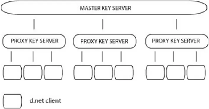
Distributed.net is a volunteer project for distributed computing created in 1997. The Distributed.net system, unlike the previously mentioned Condor system, lacks a general execution environment. All jobs need to be specifically tailored for the network. When a new project becomes available users need to download a new version of the software. Such a new version contains a module that allows for processing of the new project’s work units.

Distributed.net is built upon a client-server architecture. At the top of the system there is a master server which is also known as a master key server. It issues and keeps track of issued work units. Under the master server there are proxy key servers which request large blocks of work units from the master server. These large chunks, known as super blocks are split

into smaller blocks - work units, which are sent to requesting clients. The Distributed.net network architecture is illustrated in figure 2.1.1

Figure 2.1: Overview of distributed.net architecture

All jobs are centrally managed and can not be created by the clients. The clients only purpose is to serve the master key server with raw processing power. After clients’ finish processing work units they send them back to proxy key servers which in turn send them back to the master key server.

2.2

Peer-to-peer Networks

It is hard to a find single point in history, which could be characterized as the starting point of the service architecture type known as peer-to-peer. Different people would probably point out different points in history. What some may consider as a very important paper on peer-to-peer, others will tend to diminish as unimportant. What is certain is that the history of peer-to-peer networking is closely intertwined with the history of the network that is today known as the Internet.

As hard as it is to find a single starting point for peer-to-peer, it is even harder to find a starting point for the Internet. Some people find that J.C.R. Licklider’s publication of paper [3] on how interaction between humans can be enhanced by creating computer networks, is a stepping stone of Internet. Licklider was the first chief of Defence Advance Research Project Agency, also known as DARPA. The predecessor of today’s Internet, ARPANET was launched by the agency in 1969. ARPANET had several services that had peer-to-peer like functions and thus can be considered as a stomping ground of peer-to-peer architecture.

2.2.1

Service Architectures

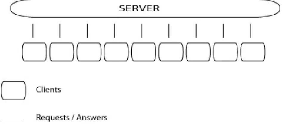
Network services can roughly employ two different architectures for commu-nication between computers on the network. The first architecture type is known as client-server architecture and is widely employed on the Internet today [6]. The main characteristic of client-server services is its distinction between service providers, known as servers, and service requesters, known as clients. Usually there are a few big servers and many small clients. This can be seen in figure 2.2. At the top is one, big server that handles requests from many clients.

Figure 2.2: Client-server network

The easiest way to understand client-server architecture is to look closely at the media situation in today’s society. There are few content providers (TV stations, newspapers, etc) and there are many content consumers (reg-ular people). This is exactly the structure that the client-server architecture in different computer services mimics. Few servers (content providers) and many clients (content consumers). Depending on what type of service you want to create you might find this mimicking good or bad. Generally services that intend to provide information from centrally managed repositories are well suited for client-server architectures.

One such example is the Network File System or NFS [14]. NFS was introduced by Sun Microsystems in 1982 and has as its primary goal to allow effective sharing of files from a central location. This gives several advantages to NFS users. Among others, it decreases storage demands and allows for centrally managed data files. Figure 2.3 contains a simplified interaction between NFS client and file server.

Figure 2.3: Communication between NFS server and client

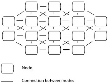
In contrast to client-server services, peer-to-peer services do not create an artificial difference between servers and clients. All computers on peer-to-peer network are equals and can both provide and request information. A real world equivalence of this architecture is ordinary people meeting each other in a town square. They can either choose to talk to (provide content) or to listen to (download content) other people. This is illustrated in figure 2.4.

Figure 2.4: Peer-to-Peer network

It is important to notice that the border between these architecture types is not sharp. Different experts are going to give different answers when asked what exactly peer-to-peer is. With the arrival of new services this border is going to get even more blurred.

2.2.2

Internet History Through Different Architectures

Services used on ARPANET were usually built with client-server architec-ture. Although this architecture was used, hosts did not act only as clients or servers, which is the case with most of the hosts on today’s Internet. Hosts on ARPANET were usually both servers and clients. Computers would usually act one time as clients, just to assume the role of server next time someone was accessing the computer. Usage pattern between hosts as whole was sym-metric [6]. Because of this early Internet is usually considered as peer-to-peer network.

ARPANET quickly became popular and started growing immensely. Ex-plosive growth radically changed the shape of the network. What started as a network between few computing sites became a natural part of every home in the developed world. This growth was not only positive. Several prob-lems appeared. Most of these probprob-lems caused the Internet to become less open. Less open networks favour client-server type services over peer-to-peer services. Below is a list of some of these problems.

Unsolicited advertisements, otherwise known as spam were literally un-known on Internet before the Internet boom in the early nineties. Today they have overrun early peer-to-peer like services as Usenet. Lack of accountabil-ity in early peer-to-peer services as Usenet and e-mail make them a popular target for unscrupulous people that send out spam.

Another change that appeared in the early nineties was decreased reach-ability between hosts. Originally every host on the Internet was able to reach every other host. A host that can reach the Internet was also reachable by computers on the Internet. This suited well symmetric usage patterns that dominated on early Internet. This was about to change in the early nineties. Firstly, system administrators started deploying firewalls, which are basically gates between different parts of networks. With the help from firewalls the system administrator can control the traffic flow to, and from the Internet. Usually they allow users on internal networks to reach the Internet while they disable access from the Internet to computers on local networks. This is done to increase security level on internal networks and is as such a very useful tool. Another change that affected reach-ability on the network was the deployment of dynamic IP addresses. Because of shortage of IP

addresses dynamic IP assignment became norm for many hosts on Internet. An individual computer receives different IP addresses by its Internet service provider (ISP) every time it connects to the Internet.

As mentioned previously all of these changes favoured client-server archi-tecture type for services over peer-to-peer like services. This caused Internet usage patterns to change from symmetric to asymmetric. Many users down-loading data and few, big service providers.

Then in the late nineties interest in peer-to-peer like services surged again. It was mostly fuelled by the success of Napster. In the wake of the Napster trial and shutdown of the original Napster network, several more or less successful peer-to-peer services followed.

2.2.3

Related Works

The next four subchapters are going to examine four different peer-to-peer like services. The first two, Usenet and DNS were services that already appeared on early Internet while the other two, Napster and Gnutella are latecomers to peer-to-peer world.

Domain Name System

The Domain Name System or DNS [11] [13] for short was introduced in 1983 as an answer to the Internet’s growing problems. Originally every host on the Internet contained a flat text file known as hosts.txt. This file contained the mapping between IP addresses like 130.236.100.21 and more user friendly names like nsc.liu.se. This file was copied around the Internet on regular basis. Managing this file became more and more tedious as Internet grew from few hosts to thousands of hosts. At the end, maintaining a accurate host list became almost impossible. DNS was the answer to this problem.

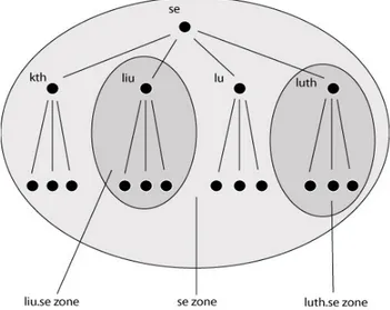
With the introduction of DNS, several peer-to-peer like structures ap-peared. Firstly, DNS introduced a hierchical system for storing records about hosts on the Internet. There is no single host that contains information about all the other hosts. Thus there is not a single failure point as is the case in client-server systems. The name servers at Link¨oping University are responsible for host names in liu.se zone. They do not have any authorative information about any other zones. If there is a hypothetical power outage at Link¨oping University that affects the name servers, only host names under liu.se are not going to be resolvable. This power outage is not going to

dis-able name resolving of hosts outside liu.se zone. Figure 2.5 contains simple illustration of different zones on Internet.

Figure 2.5: DNS Zones

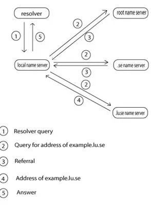
When a user types a host name in his web browser, his computer is going to try to translate the host name into an IP address. His computer contacts its local name server and supplies it with a host name it needs to resolve. It is assumed that the host name that is being searched is example.lu.se. Now the local name server contacts a root name server and asks him about the IP number of example.lu.se. As an answer it receives a referral to a name server that is responsible for the se zone. The root name server does not know the IP number of example.lu.se, but it knows that the se name server knows more. The se name server can not resolve searched host name either so it sends a reference to the name server that is responsible for the lu.se zone. Finally the name server at lu.se can answer the query. The local name server receives the answer and sends it back to the user’s computer. This process is illustrated in figure 2.6.

Another peer-to-peer like structure that DNS introduced is caching of data. The above mentioned local name server is not going to throw away the mapping between example.lu.se and IP address after sending the answer to the requesting user. It is going to keep the data for some time. This is done in case that some other user requests this information again. Next time someone requests this data, the local name server is going to be able to

Figure 2.6: DNS Query

answer directly without having to query other name servers. Data is moved close to the requesting computer. This reduces load on the name servers and the amount of data traffic flowing in and out from name servers.

Usenet

Usenet [2] was for a long time one of the Internet’s most popular services. It is still in use today although its popularity has decreased. This is one of the services that has been greatly hurt by the tremendous growth of spam. Users on the Usenet network can post their messages in different groups, which are also known as news channels. These messages are then spread among different Usenet hosts who choose which news channels they want to subscribe to.

Introduced in 1979, Usenet originally used Unix-to-Unix copy protocol (UUCP) [9]. Computers running UUCP would automatically contact and exchange messages with each other. Today Usenet has switched to a TCP/IP based protocol known as the Network News Transfer Protocol (NNTP) [10].

NNTP implements several peer-to-peer like functions. For example every message stores in its header, the path it has taken. If news server A sees that a message has already passed through news server B, it is not going to try to send the message to news server B.

Napster

Napster is a proprietary file sharing service that allowed users to swap their music files with each others. It is probably the main reason that peer-to-peer architecture experienced a revival in the late nineties. This document describes the original Napster software that allowed users to swap their music files with each other. After various legal troubles this version 1 of Napster was closed in February 2001. The software was rewritten and released as Napster v2.0 which is essentially an online music store. As Napster was proprietary software and not freely available this chapter had to be based on reports [5], [4] written by people that had reverse engineered the protocol. These reports are not official and may or may not contain errors.

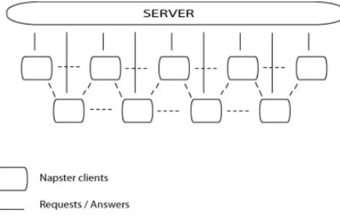
Napster uses a dual architecture network for distribution of music files. It is an example of the previously mentioned systems that blurs the line between peer-to-peer and client-network architectures. File indexing in Napster net-work is done via a simple-client model while file exchange is handled directly by the peers on the network. This model, which is pictured in figure 2.7, is also referred to as a centralized peer-to-peer service.

To gain access to Napster network the user needs to register first. Reg-istering is done automatically from the Napster client. User names on the Napster network are unique and are used in conjunction with a password to uniquely identify every user. This identification is done by Napster server. After successful logon onto the network, clients automatically upload their list of shared files to the main Napster server. The server indexes this file list into its database. When a specific client needs to find some file it issues a query to the Napster server. The server parses its database. In case the file is found, the file location is returned. The client is now free to request the searched file from the peer that has it. The download procedure varies a bit depending on if the peer with the requested file is firewalled or not. Gnutella

Gnutella is an example of a decentralized peer-to-peer service. Unlike Nap-ster there is no central repository of information on the Gnutella network. Searching and downloading is completed by peers on the network querying its neighbours. This description is based on the draft of Gnutella Protocol Specification 0.6 [12].

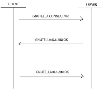
The Gnutella network is usually referred to as GNet [12]. Nodes partici-pating in GNet are referred to as servents, which is a contraction of SERver and cliENT. Because the Gnutella network lacks any fixed structure, servents need to get the host address of at least one other servent to be able to connect to the network. Finding out servent addresses can be done in two different ways. The servent can save peer addresses while present on the network and then use them next time it connects or it can use the GWebCache protocol which allows the servent to retrieve host addresses by sending simple HTTP queries to special GWebCache servers. After the address is obtained the servent connects to the network. Figure 2.8 contains a simplified handshake between a servent connecting to the network (client) and a servent already on the network (server).

Because of the lack of a central repository for information, Gnutella is almost impossible to shut down. The way the Napster service was shut down after Napster Inc. lost their case against RIAA (Recording Industry Asso-ciation of America), would be impossible with Gnutella. This is Gnutella’s greatest strength, and at the same times its greatest weakness. Although the lack of a central directory server makes Gnutella harder to shut down,

Figure 2.8: Gnutella handshake

it harms its performance greatly. Searching on decentralized peer-to-peer systems is simply never going to be on par with searching on centralized peer-to-peer systems.

If a servent on the network needs to find a specific file it issues a query message. This query message is sent to all of the servent’s neighbours. Neigh-bours in turn forward the message to their own neighNeigh-bours. This way the message is transported across the network. Usually after the message has been forwarded seven times it is discarded. Every node that receives a query message checks for the requested file and answers in case that they have the file. The requesting servent can now start downloading the file.

Chapter 3

Theory

This chapter is going to present a full description of the network that satisfies the requirements set in chapter 1. A system for distributed computing can be divided into four parts. These four parts or layers are:

• Communication • Brokering • Security • Execution

The Communication layer concerns itself with how peers connect to the network and how they communicate with each other while being on the network. It also provides a mechanism to protect the network from fragmen-tation and provides a foundation for distribution of jobs across the network. This layer is the one that fulfils the first of the three requirements of this thesis - no central points in the network. The next subchapter contains a full explanation of the communication layer.

The brokering layer handles matching of jobs and machines. It includes the matching algorithm and an XML based language for description of jobs and machines. This layer fulfils the second requirement of this thesis - full brokering capabilities. Like with the communication layer there is a sub-chapter that describes this layer.

The security layer handles the security of the system. Together with the execution layer it fulfils the third and final requirement of this thesis - full

security for the users of the system. The subchapter that describes this layer contains a formal examination of the threats and presents possible solutions to these.

The final layer - the execution layer handles execution of the jobs. It is partly described by a subchapter on security and partly described in the chapter that describes implementation of the network.

3.1

Communication

One of the requirements set for this system was lack of centralized points. Thus the main characteristic of the network that the system is run on has to be a lack of any centralized points. Such networks are usually called peer-to-peer networks. This network needs to be created for the purpose of distributing jobs.

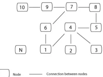
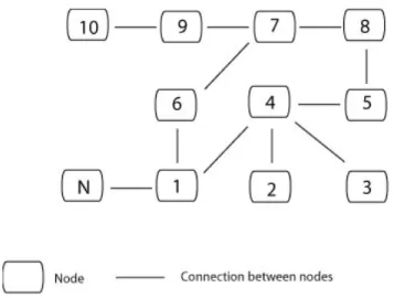
The easiest explanation of how such a network is created is through ex-amples. Thus there is going to be an extensive use of examples and figures in this subchapter. Figure 3.1 contains an illustration of a sample peer-to-peer network with ten nodes. This sample network is going to be used as the base of many hypothetical situations that are going to be examined in this subchapter. Nodes one to ten are connected to each other. Node N wants to join the network. To do this, node N has to know the address of at least one node already present on the network.

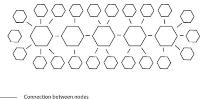
Each node, already present on the network, is connected to one or more nodes. The owners of the nodes are the ones that decide how many nodes their own computer should be connected to. The general rule is that more connections to other nodes means more traffic. Nodes with low bandwidth to the rest of the world should minimize the amount of connections and hence minimize traffic flowing into the node. On the other end, by minimizing the number of connections, the owner increases the risk of his or her node being cut off from the network. For node 2 in figure 3.1 only node 4 has to disappear for it to be cut off from the network. If node 4 is to be cut off, four different nodes have to disappear. A greater amount of connections means also that a node can reach a greater number of hosts in fewer hops. In figure 3.1, node 4 can reach six nodes in two hops, while node 2 can only reach 4 nodes in the same amount of hops. Thus nodes with high bandwidth should preferably have many connections. Making high-speed nodes prefer having many connections has one pleasant side effect - creation of a backbone of high-speed nodes. This is illustrated in figure 3.2. High bandwidth nodes are located in the middle of the network while low bandwidth nodes are on the fringes of the network.

Figure 3.2: Network with high and lowbandwidth nodes

This structure is automatically created because high-speed nodes are go-ing to strive to have many connections. This gives them benefits - high connectivity and decreased risk of being cut off from the network. At the same time low bandwidth nodes strive to be on the fringes of the network to avoid having too much traffic.

3.1.1

Finding Hosts

Like with Gnutella, there is no fixed structure on the network. Thus to connect to the network, the new node N in figure 3.1 has to know the address of at least one node already present on the network. Every node, aspiring to connect to or already connected to the network, stores a list of addresses of all known hosts. Nodes aspiring to connect to the network are going to check this list for entries. They are randomly going to choose one entry and try to connect to it. In the case of a failure, the connecting node is going to fetch a new entry and try instead to connect to that node. In the example from figure 3.1, it is assumed that node N’s list of known hosts only contains one entry - the address of node 1. Thus to connect to the network node N will have to connect to node 1. After connecting to the network, nodes can expand their known hosts list either by asking other hosts or by listening to the packets traversing the network.

3.1.2

Establishing Connection

All nodes on the network have three tables that are of vital importance to the connection procedure. First of these three tables is the one already mentioned above - the list of all known hosts. As it is said, it is a list that contains the addresses of all hosts known to the owner of the list. The second of these tables is the list of permanently connected nodes. For example node 4 in figure 3.1 has nodes 1, 2, 3 and 5 in this list. Packets that are travelling on the network are forwarded and received from these nodes. And finally, the third table is the list of all temporarily connected nodes. The difference between permanently connected nodes and temporarily connected nodes is that later ones are only connected for some pre-configured time frame, while the first ones are connected indefinitely.

Nodes on the network do not accept nor forward packets to nodes that they are not permanently or temporary connected to. Packets that are di-rectly received from other nodes are discarded.

The amount of nodes one host is connected to is regulated by the owner of that host. Based on the characteristics of the host, the owner chooses if the host should connect to few or many nodes. Besides setting the maximum amount of nodes its host should connect to, owner sets also the minimum amount of nodes his or hers host should connect to. When a host exceeds the maximum size of connections, it is not going to allow any more connections.

If a node on a network is connected to less nodes than the maximum size of connections allows, and at the same time is connected to more nodes than the minimum amount of connections, that node is not going to actively search after new nodes to connect to. Such a node is passively accepting connections. When the amount of connections falls under the value for the minimum amount of connections, the node starts actively searching for other nodes to connect to. This is the reason that the value for the minimum amount of connections is sometimes also referred to as the threshold between actively searching for and passively accepting connections. If the sample network in figure 3.1 is used again and there is assumption made that node 4 accepts at most five connections while the threshold value is three, node 4 is not going to connect to more than five nodes. At present it is also not going to try to connect to more nodes. Node 4 is already connected to four other nodes and that value is above the threshold value between passively accepting and actively searching. If node N tries to connect to node 4, node 4 is going to accept the connection. If node 2 and 3 somehow disappeared from the network, node 4 would switch to active mode and start trying to establish more connections.

3.1.3

Permanent Connections

To be able to explain the difference between permanent and temporary con-nections, there is again going to be an extensive use of the sample network in figure 3.1. It is assumed that node 1, which is connected to two other nodes, is allowed to connect to maximum three other nodes. Thus it is accepting new connections but is not actively searching for them. Threshold value is two.

Node N is, as can be seen in the figure, not connected to any nodes on the network. It is outside of the network. Thus its permanent connection list is empty. Its list of known hosts contains only one entry - node 1. To connect to the network node N will have to contact node 1 and try to establish connection with it. Upon contacting node 1, node N for the reasons explained later provides node 1 with information on how many nodes it is connected to and how many nodes it is allowed to connect to at most.

Node 1 looks into its permanent connection list, sees that it is allowed to connect to one more node and allows node N to establish connection with it. Such a connection is called a permanent connection.

3.1.4

Temporary Connections

But what would happen if node 1 was only allowed to connect to two hosts at maximum? Would node 1 just ignore node N’s connection query? In this case N is never going to be able to connect to the network - it only knows of node 1.

Answer to the second question above is no, node 1 is not going to ignore node N’s query. As mentioned in the previous chapter, node N is in its query sending information on how many other nodes it is connected to. Node 1 notices that N is not connected to anyone else - thus N is not part of the network. Because of this, node 1, which does not have place for any more permanent connections, allows node N to connect for some short time frame. This short amount of time can be used by N to find addresses of other nodes. N can then try to connect to these nodes and become a permanent part of the network. At the time the temporary connection dies, node N is hopefully going to have a permanent connection to some other node on the network. The allowed number of temporary connections is configurable by the owner of the node. If a node does not menage to create a permanent connection before the temporary connection is terminated it can try again to temporarily connect to the same node as before.

3.1.5

Getting to Know New Hosts

After establishing a connection with node 1, N becomes part of the network as illustrated in figure 3.3.

It is assumed that the size of the passive - active threshold for node N is two. Node N is still going to be actively searching for nodes to connect to. N can find new nodes to connect to in two different ways.

The first way of finding new nodes is to listen for packets traversing the network. Via its connection to node 1, N is going to start receiving packets that are travelling on the network. N adds the originators of these packets into its list of known hosts. From there it fetches entries and asks these nodes if it can establish permanent connections with them. N is not going to be able to establish any more temporary connections. N does not have any need for those and they are not more over allowed for nodes that are already connected to the network.

The other way of getting to know new nodes is to query already connected nodes. For example, N can ask node 1 for its list of known hosts. Upon

Figure 3.3: N is part of the network

receiving node 1’s known hosts list, node N will add it to its own known host list and try connecting to one of these hosts.

3.1.6

Maintaining Connection

Every node on the network expects to receive packets from hosts it is per-manently connected to within some given time frame. The size of this time frame can be configured manually on every host. Currently the default value is ten seconds. This might or might not be optimal. No tests have been conducted to prove that length of this time frame is optimal but it has been shown to function fine in the implementation that has been made for the purpose of this thesis. After this time frame has passed, nodes send so-called ping packets to each other. This is done to assure that nodes on the other end of the connection are still present on the network. Ping packets are not sent between nodes that are temporarily connected.

To illustrate how this work, the sample peer-to-peer network in figure 3.3 is going to be used. It is assumed that node 3 in the figure 3.3 has not received any packets from node 4 within node 3’s given time frame. Node 3 is going to notice this and send a ping packet to node 4. Upon receiving the ping packet, node 4 is going to answer and reset its timer for node 3. When node 3 receives answer it is, like node 4, going to reset its timer. In case that node 4 is unreachable or does not answer, node 3 is going to assume that node 4 has left the network and drop node 4 from its list of permanent

connections. Packets arriving from node 4 are not going to be accepted, nor are any new packets going to be forwarded to node 4.

3.1.7

Ending Connection

Connections on the network can be terminated in two ways. Nodes can either go down gracefully, which is preferred, or they can just vanish from the network.

There are many reasons nodes can just disappear from the network with-out notifying their neighbours. They can crash because of some malfunction in software or hardware, they can go down because of power failure or the system administrator could simply shut them down. When this happens, the nodes that are permanently connected to the node that has disappeared are going to notice this by not receiving any packets from that specific node. As explained in the the previous subchapter, the nodes connected to a node that has vanished are going to try to reach that node by sending ping packets to it. Because the node is gone, it is not going to send any answer. The nodes sending ping packets are not going to receive any answers and thus are going to remove that node from their list of permanently connected nodes.

When a node is leaving the network in a controlled manner it is going to send bye packet to all the nodes it is permanently connected to. The bye packet is going to contain a list of all nodes the leaving node was permanently connected to and a list of all hosts it knows. Upon receiving the bye packet the other nodes append the list of known hosts to their own list of known nodes. The receivers of bye packet also try to reach nodes the leaving node has been permanently connected to.

Contact of these nodes is not done directly with ping packets but by using the network. Ping packets that are not sent directly but forwarded on the network are called crawler pings. They are forwarded from one node to another. Among other things, crawler ping packets contain information on who is being searched, who is searching and time to live, which tells how many times the packets are to be forwarded. If they reach the node that is being searched, that node is going to answer with a ping packet. If the searched node is not reached, the issuing node is going to try to establish connections with the searched node. This is done mainly to avoid fragmentation of the network and is studied more thoroughly in example in 3.1.9.

3.1.8

Sending Request for Offers

Crawler ping packets is not the only packet type that is forwarded between nodes. Packets called request for offers (RFO) are also forwarded. Their purpose is to inform nodes that there is a job that needs to be matched to a machine. Every RFO packet contains information about the job that allows the machine that has received this packet to a involve matching algorithm and see if it satisfies the requirements set by the job issuer. Like crawler ping packets, RFO packets also contain a time to live field that terminates the packet after it has passed a certain amounts of hops.

3.1.9

Examples

Every network or system that wants to function properly all the time needs to be able to handle exceptions. In this part of the chapter several what-if cases are going to be presented. For every case there is a problem presentation and a proposed solution to that problem. As with the chapters above there is going to be an extensive use of examples and illustrations.

Fragmentation of the Network

Sometimes a network is going to consist of two subnetworks that are con-nected through one single host. This host is acting as a gateway between the networks. If this host leaves the network, network split is imminent. The network split creates two networks. Both of these networks are smaller and give its users less nodes to process their jobs on. Because of this, remaining nodes on the network will always try to avoid fragmentation and keep the network intact.

In a hypothetical situation, node 4 in figure 3.1 experiences a power failure and disappears off the network. Because of the nature of the failure, node 4 is not going to be able to notify the nodes it is connected to about its departure. The situation pictured in figure 3.4 is created.

As can be seen, nodes 2 and 3 are cut off from the network. They are not anymore part of the network. It is assumed that these nodes are low bandwidth nodes and have maximum connection size 1. They are after some time going to notice that node 4 is gone. They are going to send ping packets to node 4 but are not going to receive any answers. Node 4 is gone. After some time node 4 is dropped from connection tables. Nodes 2 and 3 begin

Figure 3.4: Node 4 is not part of the network

to actively search for new nodes to connect to. Hypothetically node 2 could try to establish connection with node 3 (or vice versa). This would lead to situation pictured in figure 3.5.

Figure 3.5: Node 2 and 3 have created their own network

As can be seen the network split has been made permanent. Node 2 and 3 do not allow more than one connection and are never going to be able to connect to the rest of the original network. There is a one network comprising of nodes 2 and 3 and the second network which contains rest of the nodes. To avoid this situation. nodes that connect to one host at most, are not

allowed to connect to the other hosts that also are only allowed to connect to one host at most. It could be argued that nodes that connect to at most two hosts should neither be allowed to connect to hosts with at most one connection to avoid situation pictured in figure 3.6.

Figure 3.6: Fragmented network

Because there have not been any extensive testing of settings there can not be any arguing on what the optimal settings are. In the network imple-mented for purpose of this master thesis, it was only prohibited for nodes with maximum connection size one to connect to each other. That was shown to work fine but should more extensive experiments show that more prohibition is needed, it can be easily implemented.

Another case of network fragmentation can happen when hosts like node 7 in figure 3.1 goes down. Node 7 is important because it is the only node that connects the subnetwork consisting of nodes 9 and 10 to other nodes. When node 7 goes down, the situation in figure 3.7 is created. Suddenly there are two networks.

This kind of fragmentation can not be avoided if node 7 disappears with-out notifying its neighbours of its departure. But in the case that the host leaves network gracefully all nodes that are connected to node 7 (in this case nodes 6, 8 and 9) are going to be notified that the host 7 is leaving and what hosts it was connected to. Now these nodes issue crawler ping packet. Crawler ping packets’ goal is to find out if network has been split into two

Figure 3.7: Node 7 has left the network

parts. If it is intact, nodes that node 7 has been connected to, are going to be reachable. In this case node 7 notifies nodes 6, 8 and 9 that it is parting the network. All three nodes issue two crawler ping packets. Node 8 looks for nodes 6 and 9. Node 9 is going to look for nodes 6 and 8 and node 6 for nodes 8 and 9. Now let’s take a closer look at the packets issued by node 6. These packets are sent by node 6 to the nodes that it is permanently connected to, in this case node 1. After being passed through nodes 4 and 5, these crawler ping packets are going to reach node 8. Node 8 is going to notice that it is the target of the one of those two packets. Node 8 answers by sending ping packet to node 6. Now both nodes know that they can reach each other. Both are part of the same network. While the answer for crawler ping targeting node 8 has been returned, node 6 is never going to receive answer for crawler ping targeting node 9. Node 6 assumes that the network has been fragmented. After this assumption has been made node 6 tries to establish connection with node 9. Two networks have been merged into one. Incorrect Configuration of Low or High Bandwidth Node

Sometimes users of the network are not going to be very computer literate. For example they can assume that their low bandwidth node can easily handle thirty connections to other nodes. Some other time they might decide that their high bandwidth node should not connect to more than one or two other

nodes. So how do those erroneous decisions affect the network?

In case of erroneous configuration of a low bandwidth node, the perfor-mance of network is not going to be seriously hurt. Nodes 2 and 3 are again assumed to be low bandwidth nodes on sample network from figure 3.1. The difference from previous examples is that the owner of node 2 decides that he should set the threshold between passive - active searching to thirty. Thus node 2 strives to connect to at least thirty other nodes. For every extra host node 2 connects to, the amount of traffic flowing from and into the node increases. After some time the network link on node 2 is going to get satu-rated. Node 2’s connection to outside world is clogged. Packets are going to be dropped and the owner of the node is not going to be able to do anything meaningful with his or her machine. Because other nodes are configured properly only node 2 is going to be hurt by this faulty configuration.

On the other end of the scale is the erroneous configuration of high band-width nodes. Instead of connecting to ten or maybe fifteen other nodes, the high bandwidth host connects to only one host. The owner does not under-stand benefits of being connected to many nodes. Like in the case with faulty configuration of low bandwidth node, this is not either going to decrease per-formance of the network as long as there are not many users who configure their high bandwidth nodes incorrectly. If there are many users who do this, network performance is probably going to degrade because of lack of nodes acting as the backbone of the network.

Keeping Resources for Itself

As with any other system with several users, there are going to be many misbehaving users. Sometimes some specific resource on the network is going to be a high performance computing node. It can be a powerful vector computer or a cluster of Linux nodes. As such it is going to be highly sought after. If it is assumed that node 3 in figure 3.1 is such a high performance node and that the owner of node 4 knows this, a problem could arise. As can be seen in figure 3.1, node 4 is node 3’s only link to the rest of the network. A Malicious owner of node 4 could configure his node not to forward any job requests to node 3. The owner of node 4 is keeping node 3 for his own computing needs. To avoid this, nodes on the network need to be able to analyse job requests. This will allow all nodes on the network to notice offending nodes and disconnect those. It is very unlikely that this problem is going to arise as high performance computing nodes are probably going

to have a fast connection to the outside world and be able to connect to ten - fifteen hosts instead of just one. Even if this is not likely to happen it is important that the network can handle situation like this no matter how unlikely it is.

3.2

Brokering

Every machine which is participating as a node on the network contains a description file. This file describes what resources a specific machine has to offer to different jobs and what requirements it poses on jobs that want to execute on that specific machine. For example how fast the clock speed of CPU is or the amount of Random Access Memory (RAM). It is not necessary for a description file to provide true values. A specific machine might have 512MB of RAM, but the owner wants only to allow jobs that do not require more than 256MB of RAM. Thus the owner specifies 256MB of RAM in the machine description file. As every machine’s requirements are described by a machine description file so is every job submitted to the network described by a job description file. This file is similar to machine description files but describes job properties and requirements instead of machine requirements. The following chapter contains a description of machine and job description files. It also contains a description of how a user submits jobs to the system.

3.2.1

Job and Machine Descriptions

Before submitting a job, a job specification needs to be written. The job specification is written as a job description file. This file needs to follow the rules defined in a W3C XML Schema [16], which can be found in appendix A. This XML Schema contains all the rules and requirements necessary and should be as such studied carefully by the network users. As it is a plain text file, job descriptions can be written in simple text editor, for example jed on UNIX systems or notepad on Windows. The machine description file is also a plain text file and follows exact the same rules as job description file.

Before becoming part of the network every node reads its own machine description file. Thus machine description files need either to be written by the user and made available for node on upstart or the node needs to be able to check the machine’s properties on upstart. This checking of machine prop-erties is done in different ways on different operating systems. For example

on Linux machines the node could parse /proc directory, gather necessary information from there and create machine description file automatically. A machine description file can look like this:

Figure 3.8: Machine description file

3.2.2

Rules

As was mentioned earlier, the XML Schema in appendix A defines rules for job and machine description files. The syntax of machine and job description files is heavily influenced by previous work in this area, specifically Condor’s ClassAd mechanism [1] [15], which is briefly described in chapter 2 and SSE draft. Upon reading the machine or job description file the node is going to check validity of these files against schema in appendix A. The validation of the file is done at the same time as the parsing of a description file. Node’s machine description file together with job description files provides necessary requirements for making matching of jobs and machines possible. The job specification contains all the information that the nodes on the network are going to need to successfully execute the job should they choose to accept that specific job.

Job description files consist of two parts. The requirement part specifies job requirements and preferences, while the environment part specifies all the information needed for successful execution of the job. While the job specification consist of two parts, machine description files do not need the environment part and consist only of the requirement part.

The requirement part contains machine and job requirements and pref-erences. Everything placed between <requirement>and </requirement>is considered as part of the requirement part. As can be seen from figure 3.8 the requirement consists of several nested tags that in turn also consist of several other nested tags. These tags are defined in the XML Schema in appendix A. Every valid tag in the requirement part must contain two tags

inside them and can optionally contain one more tag. The tags ”value” and ”operator” are obligatory while the tag point is optional. Here a follows short explanation of these three tags.

The value tag is as previously mentioned obligatory and nested inside every tag that is part of the requirement. In case the tag value contains a non-string value, the tag is required to have the attribute ”unit”. This attribute allows different users to use different units when specifying job and machine properties. For example a node owner can express his machine CPU clock speed in MHz while the specification for job CPU clock can be written in GHz. Thus 0.5 GHz and 500 MHz represent same value. The conversation of different units is done automatically by the system.

The ”operator” tag is also an obligatory part of all the tags that are part of the requirement. Its value can be one of following six

• equal • not equal • less than

• equal or less than • greater than

• equal or greater than

With the help of these six operators, a job can be matched to a machine. Lastly, tags in the requirement can contain the tag ”point”. With the help of the ”point” tag the job issuer can express his or her preferences. For example the user can state that his job can be executed on machines with 128 Megabyte or more of RAM. For every additional 10 Megabytes of RAM that the offering machine has to offer, it is to be ”awarded” some amount of points. In the following example:

<cpu> <value unit="MHz">500</value> <operator>eqmt</operator> <point per="100">10</point> <\cpu> <ram>

<value unit="Mb">128</value> <operator>eqmt</operator> <point per="128">2</point> <\ram>

job specification awards offering machine with 2 points for every additional 10 Megabytes of RAM. In the same example every additional 100 MHz of CPU clock speed are awarded 10 points. If two machines, the first one with following preferences: <cpu> <value>600</value> <operator>eqlt</operator> </cpu> <ram> <value>138</value> <operator>eqlt</operator> </ram>

and the second one with these preferences: <cpu> <value>800</value> <operator>eqlt</operator> </cpu> <ram> <value>128</value> <operator>eqlt</operator> </ram>

answer a job request, the job issuer is going to compare these two machines according to his preferences. The first machine is going to receive 12 points while the second one is going to receive 30 points. Machine number two has more points than machine number one. Thus machine number 2 suits the job issuer better and is chosen to process the job.

Environment tags denote the part of the job specification that contains information on the environment needed for the successful execution of the job. Inside the environment part three different tags can occur

• download • upload • execute

The ”download” tag specifies the path of a file or directory that should be downloaded and the name of that file or directory on the system after it has been downloaded. For example

<download>

<name>localName</name>

<path>ftp://example.com/someFile</path> </download>

specifies that file someFile on FTP host example.com should be downloaded and then renamed to localName after it has been downloaded. The envi-ronment part can contain several download tags. In that case all files are downloaded. Downloading of files can be done in different ways. In the above example the file was to be downloaded from an FTP server. Nodes can also use different protocols as HTTP or TFTP to download files.

The ”execute” tag can only occur once in a specific environment tag. It specifies which file should be executed after downloading all files. Usually, a file to be executed is a simple shell script that initializes all the variables required by the job and then starts the job. Usually the ”execute” tag looks like this:

<execute>localFileName</execute>

Finally after finishing the job, node looks at the upload tags. Upload tags have similar syntax as download tags. They consist of the name of a local file and the path to which the file should be uploaded. For example

<upload>

<name>localFile</name>

<path>ftp://example.com/remoteFile</path> </upload>

specifies that the node should connect to the FTP server example.com and store the file localFile there as remoteFile. As with download, different pro-tocols can be used for uploading and several files can be uploaded by using multiple upload statements.

After writing the job description file, the user is ready to submit a job. The user submits a job from his or her local node (henceforth L). L parses the job description file and creates a request for offer (RFO) packet. Besides containing information from the job description file, RFO packets have four more fields. A Unique packet identification number (UID), a Time to live (TTL) field, contact information for node issuing job request and contact information of node the forwarding this packet. After node L has created an RFO packet it sends it to all of its neighbouring nodes.

Upon reception of this packet node N that is neighbour to L examines the packet UID. This is done to avoid processing packets that have already been processed once. It also prevents loops in the network, where the same packet is sent around several times. In the case that the packet UID matches UID of some other packet that has already been received, N is going to discard the packet. Otherwise the packet is kept.

After checking the packet UID, N examines the TTL field. This field is usually initiated to between seven and ten by the job issuer (in this case L). Every node that receives the packet decreases this field value by one. Thus L decreases this packet by one also. In the case that TTL field value is zero or less the packet is discarded. As can be seen in figure 3.9, the size of the TTL field decides how many hosts are going to be reached by the request.

If the packet has passed both of these aforementioned checks, node N is going to pass the packet to its neighbours. The packet is not sent to L because L is the node that sent the message to N and thus has this RFO packet already.

After sending the packet, node N is going to check its own status. There are three possible states for every node on the network. These are

• available • matching • working

Available means that the node is not doing any work and can accept jobs should they match the node’s preferences. Matching means that the node is

Figure 3.9: High TTL increases range of the packet

currently invoking the matching algorithm or has matched a job to itself and is waiting for the job issuer to answer. In the case that the job issuer does not answer in some pre-configured time frame, the state of the node is going to be reverted back to available. When the node starts to process the job its state is changed to ”working”. If while checking its status, node N finds out that the status is ”working” or ”matching” it is not going to do anything. If status is ”available” node N is going to invoke the matching algorithm.

The matching algorithm is a piece of code that decides if both machine and job requirements can be met. The match is said to be successful when both machine and job requirements have been met. The matching of job to specific node is done in two steps. First, a node that has received job request in form of the RFO packets checks if both machine’s and job’s requirements are satisfied. If both have been satisfied, the node answers to the job issuer. Now the job issuer applies the matching algorithm again to verify the job applicant’s claims. If they are verified, the job issuer stores information about the successful job application and the number of points the job applicant received. The job issuer does not immediately answer to first successful job applicant. Instead it waits for some pre-configured amount of time so that nodes that made a successful match have enough time to answer. This allows even nodes that are located far away (on the network) to be treated fairly.

After this time frame has passed, the job applicant that got the highest value according to the point mechanism is chosen to process the job. The process in which a specific node switches between these three above mentioned states is illustrated in figure 3.10.

Figure 3.10: Rules for switching between different node states

The matching algorithm on nodes that are issuing the job and on nodes that are applying for a job works in a similar fashion. Job description files allows the user to define name of the specific resource that is requested. It also allows them to define how much of that resource is needed. For example the following job description file:

<os> <value>linux</value> <operator>eq</operator> </os> <cpu> <value unit="MHz">1500</value> <operator>eqmt</operator> </cpu>

requests that the operating system on node that is applying for the job must be Linux and that the CPU clock speed should at least be 1500Mhz. The user who has written example above, has made clear that a match can only be made if the job applicants have values for CPU clock speed and operating