Will the Asian countries buy up the United States? : Current account imbalances and the Uncovered Interest Rate Parity: Japan, China and the U.S. 1970-2008

Will the Asian countries buy up

the United States?

Current account imbalances and the Uncovered Interest Rate Parity:

Japan, China and the U.S. 1970-2008

Bachelor thesis within Economics Author: Rytis Makauskas

Tutor: Lars Pettersson, Therese Norman Jönköping 06-2012

Bachelor Thesis in Economics

Title: Will the Asian countries buy up the United States? Current account imbalances and the Uncovered Interest Rate Parity: Japan, China and the U.S. 1970-2008

Author: Rytis Makauskas

Tutor: Lars Pettersson, Therese Norman

Date: June 2012

Subject terms: Current account, Mundell-Fleming model, uncovered interest rate parity, financial account.

Abstract

This paper aims to explain the current account imbalances between the United States of America, Japan and China. According to theory, such imbalances should offset each other so that the international balance of payments account is zero. The study also tests the Uncovered Interest Rate Parity (UIP) theory for the same sample of countries. The focus is on the empirics of the topic, therefore time-series analysis is used. The results suggest that American current account deficit can indeed be explained by the surpluses of the Japanese and Chinese current accounts. Furthermore, the conclusion regarding the UIP is that it simply does not hold in the real world. Finally, the main implication of this study is that the Asian countries will eventually buy up American assets if the trend of imbalances continues.

Table of Contents

1

Introduction………...4

1.2 Purpose, limitations and outline………..……….…………..…4

2 Background………...5

2.1 Post Bretton-Woods system………...5

2.2 Historical context………...…..6

3 Theoretical Framework…..………7

3.1 Literature………....….10

4 Empirical section…………..………....11

4.1 Data description and methodology………....…12

4.3 Regression Model for Exchange rate prediction by Interest Rate Parity theory (UIP)...12

4.4 Additional regression model on the U.S. and China (UIP)……..…..13

5 Results and analysis……….……..….13

5.1 Current Accounts………...13

5.2 Uncovered Interest Rate Parity………...…14

5.2.1 United States and Japan………..…...…14

5.2.2 United States and China………..……...…15

6 Implications……….………...16

7 Conclusion……….……….……...19

References……….…...20

Appendix……….…...22

4

1 Introduction

The importance and implications of exchange rate fluctuations have been widely discussed in the academic world (Meese, R.A., Rogoff, K., 1983). Even though the exchange rate is only a number for most people, it surely affects economies and policy-making decisions worldwide. In a globalized world with enormous volumes of trade and economic integration, a country usually finds itself powerless to protect its own

economy due to openness to trade or, more generally, economic exposure. Weaknesses of economic interdependence are especially evident during external shocks and crises, when current account comes into play.

A current account is a part of the balance of payments accounts and indicates country's external position, that is whether a country is a net debtor or net creditor to the rest of the world. Soon after the breakdown of the original Bretton-Woods system, global imbalances started to deteriorate sharply. In 1971 the U.S. government, followed by most of the world's economies, abandoned the gold standard and started the era of floating exchange rate regime.

Many countries started manipulating exchange rates through open market operations to lower the value of their currencies and help the export sector, because depreciation makes domestic goods and services cheaper for foreigners, while appreciation does the reverse. Interestingly, the three countries examined in this thesis – the United States of America, Japan and China – experienced the phenomenon which contradicts the usual economic theory. Over the years, the U.S. saw its currency depreciating together with a downward trend in its current account balance, while Japan’s yen appreciated and the country accumulated large current account surplus. China followed somewhat similar pattern as Japan when it comes to the current account, but its currency, yuan, was fixed by the government for a long period of time.

The importance of the topic should be understood in an international context, i.e. large current account imbalances lead to distribution of domestic and foreign assets. As it will be shown in Section 5, due to huge and persistent current account deficit the U.S. is losing its ownership of domestic assets to Asian and oil-exporting countries. In addition, current account imbalances generally have direct and indirect implications on other economic variables. Furthermore, according to the results of this study, the Uncovered Interest Rate parity does not hold for the chosen countries. On the other hand, it still provides basic understanding of the underlying mechanisms and could be used to estimate the nominal exchange rate levels.

1.2. Purpose, limitations and outline

The purpose of this thesis is to analyze the long term imbalances of Japanese, Chinese and American current accounts in an international context, and to test whether the Uncovered Interest Rate Parity holds. These countries are the major players in the world economy these days, although the emphasis in the study is put on Japan and the U.S. because the tension between them in the 1970s-1980s has many similar implications for the current tension between the U.S. and China. The period under study spans for 38 years (1970-2008).

5 Curious readers might wonder why the euro zone is not included in the analysis. The reason is that the euro was introduced in 1999, therefore the data covers a period of only 9 years which is too short to draw any meaningful conclusions. However, this limitation does not change the results of the analysis, although it would be interesting to include the euro zone in future studies.

The outline of the paper is as follows. Section 2 provides a brief discussion on the background of the topic together with historical context. Section 3 introduces the main theories that are relevant for analysis. This part also reviews the previous studies within the field and briefly provides the reader with the most important findings. The following section is devoted to the models used in the analysis. Section 5 presents the results from the regressions, while Section 6 is focused on the implications. Finally, the last part of the paper provides concluding remarks.

2

Background

2.1. Post Bretton – Woods system

The Bretton-Woods system was an international monetary management system in which countries pegged their currencies to the U.S. dollar, which in turn was fixed at $35/ounce level. Throughout the duration of this system (1944-1971) the U.S. was flooding the world with dollars, especially in the late 1960s, when it got involved into the Vietnam War and saw its gold reserves depleting from $25 billion in the 1940s to only half of that level in the mid-1960s (Eichengreen, 2004). In addition, at that time France started to convert dollars back into gold as the uncertainty about the U.S. ability to back up the dollar presented itself. The crucial point was in 1971, when President Nixon announced that the U.S. will no longer convert dollars to gold as its gold

coverage decreased from 55% to 22%. This is known as the Nixon Shock and the end of the Bretton-Woods international monetary system.

The Post-Bretton-Woods system can be summarized by having relatively flexible exchange rates between the major currencies, active bank interventions in the markets and some fixed level of exchange rates for the newly industrialized economies (Meese, R. 1990). The transition period in the 1970s was marked by countries leaving the Bretton-Woods system by converting dollars to gold which meant nothing but further gold reserves depletion for the U.S. These events obviously had an impact on the stability of the international financial system and, to some extent, credibility of the U.S. After the breakdown of the Bretton-Woods system, the regime of floating exchange rates was introduced.

The system of floating exchange rates should, theoretically, mean the absence of

reserves in general, because balance of payments surpluses and deficits should not arise. However, countries still used it to prevent speculative attacks on currencies. After the Asian crisis in the late 1990s, the Asian governments agreed to peg their currencies to

6 the dollar and keep their reserves in dollars. This development led to increasing Asian current account surpluses and American deficit – the problem of current account imbalances which we observe nowadays.

2.2. Historical context

The 1970s were marked by two oil crises that struck the world. Not long before the first oil crisis in 1973 Japan became a modest net creditor to the rest of the world – a trend that is evident up to these days, although on a much larger scale. An increasing current account surplus was coupled with a 37.7% appreciation of Japanese yen throughout the 1970s. However, appreciation during this period was not smooth. Two oil crises, namely in 1973 and 1979, slowed the appreciating yen.

The 1980s were a period of the United States becoming net debtor of the world, and Japan being its net creditor. The U.S. trade deficit was a hot topic and eventually led to the Plaza Accord in 1985, resulting in an agreement to devalue the dollar to improve the U.S. current account condition. However, it failed to alleviate trade deficit with Japan as American exports were unable to gain grounds in Japanese domestic market due to its restrictions on imports. Furthermore, Japan's export-led economy suffered from strengthened yen (50% in 3 years) which in turn initiated loose monetary policy and asset price bubble in the late 1980s (Hayashi, F., Prescott, E.C., 2002).

The following decade started with 42% of Japan's total FDI going to the U.S., proving its position as the biggest creditor. As for the current account, in the middle of the 1990s the U.S. had a deficit of 1.5% of its GDP, while Japan was enjoying a surplus of 2.1% of its GDP. The first decade of the new millennium was exceptionally successful for Japan when it comes to the current account as it more than doubled in a period of only 7 years, amounting to 4.8% of Japanese GDP in 2007. On the other hand, this

development cannot be entirely attributed to exchange rate movements because it remained relatively stable during the period. Generally, according to economic theory, a country with positive current account tends to see its currency appreciating, which fits the Japanese case pretty well.

However, Japan has been suffering from deflationary pressures since the mid-1990s with interest rates at near-zero level. Deflation in Japan made it nearly impossible to decrease interest rate in the face of global crisis, when every country tried to spur economic activity by lowering them. On the other hand, the yen experienced a mild appreciation in the whole 1995-2010 period. Specifically, during 2007-2010 period Japanese currency appreciated by nearly 25% (OECD Statistics), while the interest rate fell from 0.5% in 2007 to 0.1% in 2010 (Bank of Japan Statistics). It contradicts the Mundell-Fleming model regarding interest rates but this phenomenon can be justified by taking into account the history of low lending rates in Japan.

Graph 1 below provides a starting point to get a grasp of how current accounts moved over time.

7 Graph 1. Current Accounts of the U.S., Japan and China, $ Billion, 1977-2008.

Source: International Financial Statistics, IMF.

One can immediately see that the current accounts of these countries trend in opposite directions, which means that the U.S. deficit is being partially financed by Japan. As it will be discussed later on, this phenomenon has serious implications for the balance of the global economy.

3

Theoretical Framework

According to theory, a country that is running a current account surplus is a net creditor to the rest of the world. It means that the country in question is providing resources to other economies and thus is owed money by them. On the other hand, if there is a deficit of the current account, a country is a net debtor and is investing more than it is saving for the future. Accordingly, it does not mean the deficit country is necessarily weak – it may use economic policies to boost its industry by borrowing resources from the rest of the world, which is recorded in the current account, and repay debts later, which is recorded in the financial account (Bishop, M., 2004).

To further understand the implications of current account surplus/deficit it is useful to have an insight into the composition of current account. The four components of current account – goods, services, income and current transfers – provide the ground for

analyzing where a surplus/deficit stems from.

The first three parts of current account are actual resources for an economy to function, while the 'current transfers' part is just unilateral transfers, such as aid or grants, with nothing in return. In Japan's case in 2007, almost half of its current account surplus was due to trade surplus with other countries ('goods' part of current account) - $123 billion (Bank of Japan Statistics). According to the Mundell-Fleming model with a balance of payments (BP) curve and less than perfect capital mobility, current account surplus should lead to increased interest rates and appreciated currency (Fleming, J.M. 1962, Mundell, R. 1963). Graphical presentation of the Mundell-Fleming model is given in Graph 2. -1000.00 -800.00 -600.00 -400.00 -200.00 0.00 200.00 400.00 600.00 1977 1979 1981 1983 1985 1987 1989 1991 1993 1995 1997 1999 2001 2003 2005 2007 Japan U.S. China

8 Graph 2. Mundell-Fleming model (IS-LM-BP)

IS curve: Y = C + I + G + NX, where Y is output, C – consumption, I – investment, G – government spending, and NX is net exports.

LM curve: M/P = L( i, Y ), where M is nominal money supply, P – price level, L – real money demand, i – interest rate, and Y is output. Note that higher interest rate or lower output causes lower money demand.

BP curve: BP = CA + KA, where BP stands for balance of payments, CA is current account and KA is capital account.

The IS curve represents equilibrium in goods and services market for different national income and interest rate levels; the LM curve represents equilibrium in money market; the BP curve portrays balance of payments position. If the IS and LM curves cross above the BP line, such as at point G, then there is a balance of payments surplus, whereas if they cross below the BP line, such as at point F, there is a deficit. The IS-LM-BP model is usually used to analyze monetary and fiscal policies under different exchange rate regimes. However, the relationship between current account and exchange rate in the model suggests that the current account surplus will shift the IS curve to the right, leading to the balance of payments surplus and excess demand for domestic currency, which in turn will create pressure for appreciation.

It is important to keep in mind that the magnitude of movements in the IS-LM-BP model depend on elasticity of each curve, or in other words, on country’s relative sensitivity to changes in interest rates and output levels.

Furthermore, a paper by Obstfeld and Rogoff (1996) provides an intertemporal approach to the current account. This approach is based on the notion that the current account balance is the result of future investment-saving decisions. Therefore, if the current account is essentially saving minus investment, Asian countries’ propensity to save and America’s tendency to spend will create disequilibrium of international payments. Rogoff and Obstfeld found that this approach is extremely useful in explaining the oil price shocks of the 1970s for OECD countries. What is more, they

9 extended models to incorporate relative prices, asymmetric information, complex

demographic structure, and asset-market incompleteness, and concluded that the intertemporal approach models are consistent for open-economy policy analysis and should be used together with the IS-LM models (Obstfeld, M., Rogoff, K. 1996). Another relevant theory is the J-curve theory which states that it takes time for current account balance to improve after depreciation (Demirden, T., Pastine, I. 1995). The reason is that due to sticky prices trade balance does not adjust immediately – it worsens initially and improves over time (Graph 3). The J-curve theory helps to explain the lags in current account improvement.

Graph 3. J-curve

According to the J-curve theory, if a country wants to improve its current account balance through depreciation (point X), it will see the balance worsening in the beginning (point Y) and only after some time it will improve (point Z).

Furthermore, the interest rate parity theory is crucial to analyze exchange rate

movements as it states that the interest rate differential is equal to the expected rate of depreciation (Frankel, J.A., 1979):

∆e = r – r*,

where r is the domestic interest rate, r* is foreign interest rate, and ∆e is the expected rate of depreciation. The variable ∆e could also be understood as the difference between the forward (future) and spot exchange rates of the currencies in question. According to this theory, a country with higher interest rate should see its currency depreciating. In other words, country A must offer a higher interest rate to attract investors if its currency is to depreciate in the future. This theory is also known as ‘covered interest rate parity’ because investors back their investments by agreeing on the future exchange rate in advance. If they do not back their investments by futures, then the difference between interest rates is the expected rate of depreciation (uncovered interest rate parity - UIP).

This particular relationship between current account and exchange rate has attracted much attention over the years, as the world became more interdependent than ever

10 before. Growing volumes of trade and economic integration in general made it of

special importance to research and examine the connection between exchange rate and current account. Most researchers agree that both are vital to the economy in the sense that they provide some indication about the overall condition of an economy. However, the conclusions contradict each other in some cases.

3.1. Literature

Ueda (1988) provides some explanation for the developments and connection between the current account and exchange rate in 1970s and 1980s. According to him, the current account surplus that was accumulated by Japan in 1970s induced capital outflows and gave strong pressure for the yen to appreciate. The Bank of Japan intervened in the foreign exchange market to prevent sharp swings in exchange rate. However, expectations of the yen depreciation arose after the intervention, resulting in further capital outflows. On the other hand, the 1980s were a different story. With foreign interest rates being higher than Japanese and relaxation of capital flows by the authorities, it was no surprise to see massive capital outflows to the U.S. as Japanese investors bought American assets due to favorable international conditions (Ueda, K.,1988). Ueda's explanation of the developments during these two decades makes sense, although it misses the very important Plaza Accord in 1985.

A paper on global current account imbalances and exchange rate adjustments by Rogoff and Obstfeld (2005) has some interesting insights. One of them is the connection

between the tax cuts in the 1980s by the Reagan Administration and the increasing U.S. current account deficit at the time. Another period of similar practice was during the presidency of George W. Bush when tax cuts resulted in increasing current account deficit. These events fit well into the Mundell-Fleming model with less than perfect capital mobility which portrays that fiscal expansion (tax cuts in this case) causes people to spend more money on imports, which worsens the current account (Rogoff, K. and Obstfeld, M., 2005). Interestingly, they found that currency under- and

overvaluations were followed by changes in the U.S. external position. These

developments were also relevant for Japan because of the two countries’ trade practice. It can be found that after the tax cuts in the U.S. its current account deficit soared, while the Japanese were enjoying a growing surplus.

The scholars analyzed the periods of 1981-1989 and 2001-2009 when Reagan and Bush were in office, respectively. Equipped with Rogoff and Obstfeld's reasoning and data from the IMF, one can track down the impact of the tax cuts in the U.S. on its current account balance as well as on Japan's. Of course, it would be naive to attribute the growing surplus in Japan solely to the developments in the U.S.; the way to look at it is that due to the scale of global economic integration events in one country can have specific effect on other country's position.

What is more, exchange rate adjustments also occurred during the two periods. The Reagan period was marked by a sharp yen appreciation, especially in his second term. Nonetheless, Japan's current account balance performed better during Reagan's first term in office, which was the period of big tax cuts and recovery from the recession in early 1980s resulting in consumption boom. On the other hand, the yen-dollar exchange

11 rate remained at roughly the same level (trending mildly towards appreciation, however) during the presidency of G. W. Bush while Japan's current account more than doubled since its level in 2001, reaching the peak in 2007 (Graph 1). According to Rogoff and Obstfeld, exchange rate adjustments occurred before changes in the current account balance (Rogoff, K. and Obstfeld, M., 2005).

A discussion paper by B.E.Loopesko and R.A.Johnson (1987) on realignment of the yen-dollar exchange rate provides a test on the adjustment process in Japan. They use the Federal Reserve Board staff's Multi-Country Model (MCM) to come up with simulations. The model suggests that the Japanese fiscal expansion would be less effective in narrowing the two countries' trade imbalance than the U.S. fiscal

contraction (Loopesko, B.E., Johnson, R.A., 1987). The researchers also predicted a further yen appreciation against the dollar which, as can be observed, materialized since the mid-1980s.

Yet another paper written by Wyplosz (2010) particularly examines today's hot topic of huge imbalances between the U.S. and Chinese current accounts. He argues that the source of dispute is the same as it was almost 30 years ago between the U.S. and Japan. Wyplosz uses national saving and investment approach to explain the current Sino-American imbalances and concludes that low saving and high investment in the U.S. on one hand, and high national saving in China on the other, created this disequilibrium. Furthermore, he argues that financial deregulation in the U.S. and increased openness in China widened the gap between their current accounts. Finally, he found that the U.S. budget balance and its net private saving have almost perfect negative correlation (Wyplosz, C., 2010).

Finally, a paper by Meredith and Chinn (2004) on uncovered interest rate parity

provides some explanation about why the uncovered interest rate parity usually does not hold in the real world. According to them, the exchange rates in the long-run are driven by the ‘fundamentals’, which are not included in the UIP theory. Furthermore, although the UIP explains the variation in the exchange rates better than the random walk

hypothesis, the explained volatility is still just a small part of the observed variance in the exchange rates (Meredith, G., Chinn, M.D., 2004).

It is evident from the literature that there is no ultimate answer to the current account imbalance and exchange rate problem. However, one should consider different possible conclusions provided by different approaches.

4

Empirical Section

This section provides data description and regression models that are used in order to analyze the current accounts and exchange rates predicted by the interest rate parity theory for the U.S., Japan and China. It also briefly describes the method that is used to obtain the results.

12

4.1. Data description and methodology

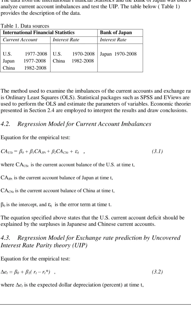
The data from the International Financial Statistics and the Bank of Japan was used to analyze current account imbalances and test the UIP. The table below ( Table 1) provides the description of the data.

Table 1. Data sources

International Financial Statistics Bank of Japan Current Account Interest Rate Interest Rate

U.S. 1977-2008 U.S. 1970-2008 Japan 1970-2008 Japan 1977-2008 China 1982-2008

China 1982-2008

The method used to examine the imbalances of the current accounts and exchange rates is Ordinary Least Squares (OLS). Statistical packages such as SPSS and EViews are used to perform the OLS and estimate the parameters of variables. Economic theories presented in Section 2.4 are employed to interpret the results and draw conclusions.

4.2. Regression Model for Current Account Imbalances

Equation for the empirical test:

CAUSt= β0 + β1CAJPt + β2CACNt+

ε

,

where CAUSt is the current account balance of the U.S. at time t,

CAJPt is the current account balance of Japan at time t,

CACNt is the current account balance of China at time t,

β0 is the intercept, and

ε

The equation specified above states that the U.S. current account deficit should be explained by the surpluses in Japanese and Chinese current accounts.

4.3. Regression Model for Exchange rate prediction by Uncovered

Interest Rate Parity theory (UIP)

Equation for the empirical test:

∆et = β0 + β1( rt – rt*) , (3.2) where ∆et is the expected dollar depreciation (percent) at time t,

13

β0 is the intercept, β1 is the parameter of the interest rate differential, rt is the interest rate in the U.S. at time t, and rt* is the interest rate in Japan at time t.

Economically speaking, the equation above states that the higher interest rate in the U.S. should lead to the dollar depreciation.

4.4. Additional regression model on the U.S. and China (UIP)

First of all, the reader should be careful when considering the model to test the UIP for China and the U.S. The reason is that the data is limited since only 26 observations are included, which is an issue when performing any kind of regression. Second, the capital flows and exchange rate were regulated by the Chinese government until 1996 (Nancy, Y.N. 2009), which also has implications for the results obtained from the regression. The equation for the regression is the same as in the previous subsection, except that r* stands for Chinese interest rate.

5

Results and analysis

This section presents the results obtained after performing the regressions. It also provides analysis to interpret the results in economic fashion.

5.1. Current Accounts

The following table (Table 2) presents OLS results, which are followed by economic interpretation based on respective theories.

Table 2. U.S., Japanese and Chinese current accounts, 1977-2008.

Dep.Var.: U.S. CA

Variable β t-stat. sign. DW R-squared

Constant 21.221 0.522 0.605 0.42 0.792

Japan CA -2.369 -4.997 0.000 China CA -1.062 -4.078 0.000

First of all, it is evident from Table 2 that both explanatory variables should be included in the model as their p-values are very low. Second, the coefficients for Japan and China are negative (-2.369 and -1.062, respectively), which means that an increase in their current account balances leads to the increasing current account deficit of the U.S. Furthermore, even though the intercept is not statistically significant, it does have an economic message behind it. The intercept in this case represents countries that are not included in the model but trade with the U.S. and have positive current account balances. It is worth mentioning that the biggest piece of the intercept would be

14 explained by the combined surpluses of oil-exporting countries – mainly OPEC members (Arezki, R., Hasanov, F. 2009). What is more, the Durbin-Watson test statistic is 0.42 which is substantially lower than 2, and says that there is serious autocorrelation. However, in this particular case it is expected because both China and Japan have surpluses in their current accounts. Finally, the R-squared is 0.792, so nearly 80% of the variation in the dependent variable (CAUS) can be explained by the variation in the

independent variables (CAJP and CACN). Overall, the results from the regression are in line with

the Mundel-Flemming model, as it is seen that current account surplus in one country transforms to a current account deficit in another country.

5.2. Uncovered Interest Rate Parity (UIP)

This subsection is devoted to the results obtained from the regression on the UIP.

5.2.1. United States and Japan

The table below (Table 3) shows the results from the regression on the UIP. The failure of the UIP is briefly discussed together with probable reasons of why it fails.

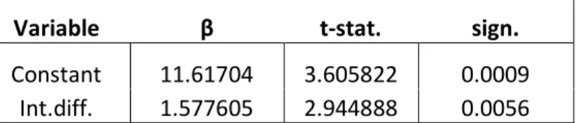
Table 3. Expected dollar depreciation, 1970-2008.

Dep.Var.: Dollar depreciation

Variable β t-stat. sign. R-squared

Constant 11.61704 3.605822 0.0009 0.194133

Int.diff. 1.577605 2.944888 0.0056

As it is seen from the Table 3, the interest rate differential for the U.S. and Japan (variable Int.diff.) should be included in the model explaining the changes in the exchange rate of these countries. The regression says that when the interest rate differential increases by 1 unit, the dollar depreciates by 1.57%. However, the model has quite poor explanation power, as only about 19% of the variance in the exchange rate is explained by the variation in the interest rate differential. It is useful to take a closer look at the plotted data to verify this (Graph 4).

15 Graph 4. Yen/Dollar exchange rate and interest rate differential, %, 1970-2008

Sources: Bank of Japan and International Financial Statistics, IMF

The results from the regression are similar to those of Meredith and Chinn (2004), who found that the UIP works better in explaining the exchange rate movements over longer time periods, but it still is a poor predictor for the future changes in the exchange rate. However, the slope parameter is of correct sign and its value is closer to 1, which is what the UIP theory states.

The Uncovered Interest Rate parity does not hold, according to these results, which might be due to fact that it does not incorporate other important variables, such as money supply, inflation and output levels (Neely, Ch.J., Sarno, L. 2002).

5.2.2. United States and China

Table 4. Expected dollar depreciation, 1982-2008.

Dep.Var.: Dollar depreciation

Variable β t-stat. sign. R-squared

Constant 5.168144 2.417464 0.0229 0.008833

Int.diff. 0.246680 0.481344 0.6343

Table 4 essentially carries the same message as Table 3, but for the U.S. and China. The results are that the UIP is weak in explaining the variance in the exchange rate by the variance in interest rate differential. In this case, it performs extremely weak as the R-squared value is very low. However, one should remember that China has been fixing the value of yuan and regulating its capital markets for a long period of time, which obviously affects the results of tests like this. In addition, low statistical significance and R-squared values are found by other scholars that analyzed the Uncovered Interest Rate parity (see Bilson (1981), Cumby and Obstfeld (1985), Chinn (2006)).

-40 -30 -20 -10 0 10 20 1970 1972 1974 1976 1978 1980 1982 1984 1986 1988 1990 1992 1994 1996 1998 2000 2002 2004 2006 2008 change% r-r*

16

6

Implications

6.1. Current accounts

The balance of payments (BP) analysis states that a deficit in one of the accounts must be offset by a surplus in the other. In nowadays international context it means that the relative balance of the international transactions is reached by the U.S. having a deficit in its current account and Asian countries having a surplus in their current accounts. The question is then ‘Can this trend go on forever?’

Apparently, it has been going for a while and the U.S. current account deficit has been financed by the surplus in its financial account (Graph 5).

Graph 5. U.S. Current and Financial accounts, $ Millions

Source: U.S. Department of Commerce, Bureau of Economic Analysis

Importantly, the surplus in the U.S. financial account implies the sales of domestic assets (see Appendix) to Japan and China primarily, and to oil-exporters, which

consequently means that the U.S. is losing ownership of its assets (Mueller, A.P., 2011). If one wants to take the discussion one step further, a question of autonomy would be next but it is out of the scope of this thesis.

Furthermore, ‘excessive’ current account imbalances may be seen as a signal of a country’s creditworthiness, especially when it comes to deficits. This is already happening as Standard & Poor’s, a credit rating agency, downgraded the U.S.’s AAA rating to AA+ in 2011 (Bloomberg, August 6, 2011). It is complicated to perform econometric analysis on the problem of solvency as there are factors such as market expectations and degree of openness, which are difficult to measure; therefore there is no clear-cut answer to the question of ‘How long can this trend go?’

In addition, the obvious suggestion for the U.S. policy-makers is to decrease the current account deficit by increasing the level of saving if they do not want to see their country

17 being owned by the Asian countries. This improvement can also be achieved through foreign direct investment (FDI) because it does not alter country’s external position (Rossini, G. et al, 2006).

However, the results from the regression suggest that further research is needed to fully explain these current account imbalances. It might be useful to include the OPEC countries into the model as the recent article in The Economist suggests (R.A., 2012).

6.2. Exchange Rates

Interestingly, the UIP fails to explain the changes in the nominal exchange rates but it at least predicts the value pretty good. Using the formula below one can calculate the nominal exchange rate at some period of time:

Et+1 = Et * (( 100 – (r-r*)) / 100 ),

where Et+1 is the nominal exchange rate in t+1,

Et is the current nominal exchange rate, and r-r* is the interest rate difference between the countries in question.

Graphs 6 and 7 represent the actual and UIP predicted exchange rates. Graph 6. Yen VS Dollar, nominal exchange rate

Source: Bank of Japan

Graph 7. Yuan VS Dollar, nominal exchange rate

- 100.00 200.00 300.00 400.00 Yen/Dollar predicted

18

Source: OECD Database

However, for the purposes of further research on the UIP one should obviously consider other factors that affect changes in the exchange rates. The article by John Harvey (2003) suggests that the risk premiums are not a necessary condition to cause the failure of the UIP. He argues that confidence-related variables, such as high U.S. debt and low growth rates, explain the biggest piece of the deviations from the UIP (Harvey, J. 2003). The UIP is a good starting point to understand the international capital flows, but it is rather intuitive that such a simple theory cannot explain our complex and dynamic world. 0 2 4 6 8 10 Yuan/Dollar predicted

19

7

Conclusion

This thesis aimed to analyze the long-term imbalances of the American, Japanese and Chinese current accounts. The results from the regression suggest that nearly 80% of the American current account deficit is explained by the surpluses in the Japanese and Chinese current accounts. However, the relative or temporary balance of international transactions cannot be sustainable in the long-run as the current account deficit implies a surplus in the financial account, which in turn means the loss of ownership of

domestic assets. This phenomenon has serious implications for the deficit country – the United States. If the trend continues, the U.S. will essentially sell its assets to surplus countries – primarily Japan and China, and also the oil-exporting countries. However, it is difficult to say when this development will happen as there are measurement

problems regarding economic variables. Finally, the U.S. should decrease its current account deficit by increasing the level of saving or attracting more foreign direct investment.

Another conclusion that can be drawn from the analysis part is that the Uncovered Interest Rate parity (UIP) does not hold, that is the interest rate differential fails to explain changes in exchange rate. On the other hand, the UIP might be used to estimate the value of a particular exchange rate. However, one should bear in mind that the predictions suggested by the UIP can only be applied in the short-run, as there are other factors that affect the exchange rates which the UIP does not account for.

20

REFERENCES

1. Arezki, R., Hasanov, F. April 2009. “Global Imbalances and Petrodollars”, IMF Working Paper 09/89.

2. Bilson, J.F.O. 1981. “The ‘Speculative Efficiency’ Hypothesis”, Journal of Business, Vol. 54, No.3, p.435-451.

3. Bishop, Matthew. 2004. “Essential Economics: An A to Z Guide (The Economist)”, Bloomberg Press; 1st edition.

4. Chinn, M.D. 2006. “The (partial) rehabilitation of interest rate parity in the floating rate era: Longer horizons, alternative expectations, and emerging markets”, Journal of International Money and Finance, Vol. 25, p. 7-21. 5. Cumby, R.E, Obstfeld, M. 1985. “International Interest-Rate and Price-Level

Linkages Under Flexible Exchange Rates: A Review of Recent Evidence”, National Bureau of Economic Research, Working Paper No.921, p. 121-151. 6. Demirden, T., Pastine, I. 1995. “Flexible exchange rates and the J-curve: An

alternative approach”, Economic Letters 48, 1995, p. 373-377.

7. Detrixhe, J. August 6, 2011. “U.S. Loses AAA Credit Rating as S&P Slams Debt Levels, Political Process”, Bloomberg.com.

8. Eichengreen, B. 2004. ’’Global Imbalances and the lessonso of Bretton

Woods’’, National Bureau of Economic Research, Working Paper 10497, p. 5. 9. Fleming, Marcus J., "Domestic Financial Policies under Fixed and under

Floating Exchange Rates," IMF Staff Papers, November 1962.

10. Frankel, J.A. 1979. “On the mark: A Theory of Floating Exchange Rates based on Real Interest Differentials”, The American Economic Review, Vol.69, No.4. 11. Harvey, J. 2003. “Deviations from Uncovered Interest Rate Parity: A Post

Keynesian Explanation”, Working Papers 200301, Texas Christian University, Department of Economics.

12. Hayashi, Fumio and Prescott, Edward C, 2002. “The 1990s in Japan: A Lost Decade”, Review of Economic Dynamics 5, 206-235, 2002.

13. Loopesko, B.E., and Johnson, R.A. 1987. “Realignment of the Yen-Dollar exchange rate: Aspects of the adjustment process in Japan”, International Finance Discussion Papers, No.311, August, 1987.

14. Meese, R. 1990. ’’Currency fluctuations in the Post-Bretton Woods Era’’, The Journal of Economic Perspectives, Vol. 4, No. 1, p. 117-134.

15. Meese, R.A., Rogoff, K. 1983. “Empirical exchange rate models of the seventies: Do they fit out of sample?”, Journal of International Economics vol.14, p. 3-24.

16. Meredith, G., Chinn, M.D. 2004. ” Monetary Policy and Long Horizon Uncovered Interest Parity”, IMF Staff Papers 51, 3 (November 2004), p. 409-430.

17. Mueller, A.P., 2011. “Balance of Payments Analysis”, Continental Economics Institute Research Paper Series 2011.

18. Mundell, Robert, "Capital Mobility and Stabilization Policy under Fixed and Flexible Exchange Rates," Canadian Journal of Economics and Political

21 19. Nancy, Ni Y. 2009. “China's Capital Flow Regulations: The Qualified Foreign

Institutional Investor and the Qualified Domestic Institutional Investor Programs”, Review of Banking & Financial Law, Vol. 28, 2008-2009, p. 299-301.

20. Neely, Ch. J., and Sarno, L. 2002. “How well do monetary fundamentals forecast exchange rates?”, The Federal Bank of St. Louis, September/October Review, p.51-74.

21. Obstfeld, M., Rogoff, K. 1996. “The Intertemporal Approach to the Current Account”, National Bureau of Economic Research, No.4893.

22. R.A. April 26, 2012. “Global imbalances: The Black Hole”, The Economist, Free Exchange blog.

23. Rogoff, K. S., and Obstfeld, M. 2005. “Global Current Account Imbalances and Exchange Rate Adjustments”, Brookings Papers on Economic Activity, Vol. 2005, No. 1.

24. Rossini, G., and Zanghieri, P. 2006. “Current account composition and sustainability of external debt”, Applied Economics 41, p. 3-7.

25. Ueda, K. 1988. “Perspectives on the Japanese Current Account Surplus”, Macroeconomics Annual 1988, National Bureau of Economic Research, Vol.3. 26. Wyplosz, C., 2010. “Is an undervalued renminbi the source of global

imbalances?”, VoxEU.org, April 30, 2010.

Data set

1. Bank of Japan Statistics, Exchange rate and Interest rate, 1970-2008. 2. International Financial Statistics, IMF, Current Accounts 1977-2008. 3. OECD Database, Nominal exchange rates, China 1980-2008.

4. U.S. Department of Commerce, Burreau of Economic Analysis, U.S. Current and Financial Accounts 1970-2008.

1. Foreign-owned assets in the U.S.

3. SPSS output for current account imbalances regression

Model Summaryb

Model R R Square Adjusted R Square

Std. Error of the

Estimate Durbin-Watson

1 ,890a ,792 ,778 120,28313 ,420

a. Predictors: (Constant), China, Japan

b. Dependent Variable: U.S

Coefficientsa Model Unstandardized Coefficients Standardized Coefficients t Sig. B Std. Error Beta 1 (Constant) 21,221 40,616 ,522 ,605 Japan -2,369 ,474 -,543 -4,997 ,000 China -1,062 ,260 -,443 -4,078 ,000

4. EViews output for UIP regressions 1. Yen VS Dollar

2. Yuan VS Dollar

Dependent Variable: CHANGE_ Method: Least Squares

Date: 05/08/12 Time: 18:28 Sample (adjusted): 1970 2007

Included observations: 38 after adjustments

Variable Coefficient Std. Error t-Statistic Prob. C -11.61704 3.221746 -3.605822 0.0009 R_R_ 1.577605 0.535710 2.944888 0.0056 R-squared 0.194133 Mean dependent var -3.282892 Adjusted R-squared 0.171747 S.D. dependent var 10.42876 S.E. of regression 9.491045 Akaike info criterion 7.389770 Sum squared resid 3242.877 Schwarz criterion 7.475959 Log likelihood -138.4056 Hannan-Quinn criter. 7.420436 F-statistic 8.672365 Durbin-Watson stat 1.566421 Prob(F-statistic) 0.005631

Dependent Variable: CHANGE Method: Least Squares Date: 05/08/12 Time: 18:36 Sample (adjusted): 1980 2007

Included observations: 28 after adjustments

Variable Coefficient Std. Error t-Statistic Prob. C 5.168144 2.137837 2.417464 0.0229 R_R_ 0.246680 0.512481 0.481344 0.6343 R-squared 0.008833 Mean dependent var 5.479137 Adjusted R-squared -0.029289 S.D. dependent var 10.62886 S.E. of regression 10.78339 Akaike info criterion 7.662641 Sum squared resid 3023.320 Schwarz criterion 7.757798 Log likelihood -105.2770 Hannan-Quinn criter. 7.691731 F-statistic 0.231692 Durbin-Watson stat 1.474229 Prob(F-statistic) 0.634298

Appendix