A branch-and-cut method for the Vehicle Relocation Problem in the One-Way Car-Sharing

(1)

DEGREE PROJECT, IN OPTIMIZATION AND SYSTEMS THEORY , SECOND LEVEL

STOCKHOLM, SWEDEN 2015

A branch-and-cut method for the

Vehicle Relocation Problem in the

One-Way Car-Sharing

(2)

(3)

Institutionen för matematik Fakultät für Mathematik

Avdelning för Optimeringslära Lehrstuhl für Angewandte Geometrie och Systemteori und Diskrete Mathematik

A branch-and-cut method for the

Vehicle Relocation Problem in the

One-Way Car-Sharing

S Z Y M O N J A N U S Z A L B I N S K I

Master’s Thesis in Optimization and Systems Theory (30 ECTS credits) Master Programme in Engineering Physics (120 credits) Royal Institute of Technology year 2015 Advisors at TUM: Dr. Michael Ritter, M. Sc. Wolfgang Riedl Supervisor at KTH: Prof. Dr. Anders Forsgren

Examiners: Prof. Dr. Peter Gritzmann (TUM) Prof. Dr. Anders Forsgren (KTH)

TRITA-MAT-E 2015:15 ISRN-KTH/MAT/E--15/15--SE

Royal Institute of Technology

School of Engineering Sciences

KTH SCI

SE-100 44 Stockholm, Sweden URL: www.kth.se/sci

(4)

I hereby confirm that this is my own work, and that I used only the

cited sources and materials.

(5)

Abstract

The purpose of this thesis is to develop an algorithm which solves the Vehicle Relocation Problem in the One-Way Car-Sharing (VRLPOWCS) as fast as possible. The problem describes the task of relocating the cars to areas with the largest demand. The chauffeurs who relocate the cars are transported by shuttle buses. Each car is assigned an individual relocation utility. The objective is to find shuttle tours that maximise in a given time the relocation utility while balancing the distribution of the cars. The VRLPOWCS is formulated as a mixed integer linear program. Since this problem is NP-complete we choose the branch-and-cut method to solve it. Using additional cutting planes – which exploit the structure of the VRLPOWCS – we enhance this method. Tests on real data show that this extended algorithm can solve the VRLPOWCS faster.

Sammanfattning

Syftet med detta examensarbete är att utveckla en algoritm som löser fördelningsprob-lemet av car-sharing bilar (VRLPOWCS) så snabbt som möjligt. Probfördelningsprob-lemet beskriver uppgiften att flytta bilarna till områden där efterfrågan är störst. Bilarna flyttas av chaufförer som är transporterade med bussar. Varje bil ges ett flyttningsvärde. Målet är att hitta resor för bussarna så att inom ett visst tidsintervall det totala flyttningsvärdet är maximerat med hänsyn till en given fördelning. VRLPOWCS formuleras som ett lin-järt heltalsprogrammeringsproblem. Eftersom problemet är NP-fullständigt, använder vi branch-and-cut metoden för att lösa det. Metoden utvidgar vi med cutting planes vilka utnyttjar VRLPOWCS strukturen. Tester med olika riktiga data visar att den utvidga algoritmen kan lösa VRLPOWCS snabbare.

Zusammenfassung

Das Ziel dieser Arbeit ist die Entwicklung eines Algorithmus, der das Umparkproblem im Free-Floating Carsharing (VRLPOWCS) schnellstmöglich löst. Beim Umparkproblem werden Carsharing Fahrzeuge in Gebiete mit der höchsten Nachfrage umverteilt. Dabei werden die Autos von Fahrern umgeparkt, welche von Kleinbussen transportiert werden. Jedem Auto wird ein individueller Nutzenwert zugewiesen. Das Ziel des Umparkprob-lems ist das Finden von Bustouren, die in gegebener Zeit den Umparknutzen unter Beachtung einer gewissen Verteilung der Fahrzeuge in den Zielräumen maximieren. Das VRLPOWCS wird als ganzahlig-lineares Optimierungsproblem formuliert. Zur Lösung des VRLPOWCS wird ein Schnittebenenverfahren verwendet, da das Problem NP-vollständig ist. Das Verfahren wird mit Schnitten verbessert, die die Struktur des VRLPOWCS ausnutzen. Testläufe mit echten Daten zeigen, dass der erweiterte Algorithmus das VRLPOWCS schneller lösen kann.

(6)

(7)

Acknowledgements

I would like to express my gratitude to all those who have enabled me to write this thesis. First of all I want to thank my two examiners, Prof. Dr. Peter Gritzmann and Prof. Dr. Anders Forsgren, who both enabled me in an uncomplicated manner to write this thesis simultaneously at both chairs. I am very grateful for the assistance and supervision given to me by Prof. Dr. Anders Forsgren. Tack så mycket!

Of equal importance was the commitment and advice provided by my two advisors Dr. Michael Ritter and M. Sc. Wolfgang Riedl. I would like to express my appreciation to both of them for their valuable and constructive suggestions during the development of this thesis. Their countless comments as well as willingness to discuss and to answer my questions were of great help.

I also want to thank Anja König for carefully reading through this thesis and pointing out errors. Naturally, any remaining inconsistencies are entirely my own.

Finally, I am much obliged to my family – especially to my parents – for their immense support and encouragement throughout my whole studies.

(8)

(9)

Chapter 1 One-way car-sharing

“The concept of using a car but not owning one.” 1

The term “car-sharing” describes shared vehicle programs which give people the pos-sibility to use temporarily a car. This idea was born in 1948 in Zurich, Switzerland, when a housing community started to commonly use vehicles in the “Selfage” program. In the next decades some more projects were initialised in Europe and the United States, but car-sharing eked out a niche existence until the 1990s [Mil+05].

The trend towards urbanisation in the recent years lead to the rediscovery of car-sharing as a solution to the changed mobility behaviour in big cities. Since the millennium years, car-sharing became more and more popular and several car-sharing companies have offered their services to a growing number of customers. In Germany, for example, the number of car-sharing vehicles grew from 1,500 in 1999 to 15,500 in 2015 according to the Bundesverband CarSharing, Germany’s national car-sharing association (see Fig. 1.1). At the begin of 2015 1,040,000 customers – 37.4 percent more than in 2014 – were registered with 150 German car-sharing providers [Bun15b]. Today, in almost ev-ery major city in Germany several providers offer their services. In Sweden, car-sharing has not been that popular although in 1983 the car-sharing program “Vivalla bil” opened in Örebro [Ber98]. However, since December 2014 a big car-sharing provider offers its services in Stockholm.

There are several models of car-sharing services, among them one-way car sharing which is very popular in Germany. In the one-way car-sharing – also called free-floating car-sharing – the car-sharing providers define zones in the city where the cars can be parked. These zones usually cover the city centre and hotspots like railway stations or airports. The customers can use web-based services to locate available cars and member cards to access them. The usage of the cars is typically charged per minute, starting at the moment when the customers open the cars and ending when they park them somewhere in the predefined zones.

1

(14)

Chapter 1 One-way car-sharing 1.500 3.500 5.500 7.500 9.500 11.500 13.500 15.500 17.500 0 100.000 200.000 300.000 400.000 500.000 600.000 700.000 800.000 900.000 1.000.000 1.100.000 1997 1998 1999 2000 2001 2002 2003 2004 2005 2006 2007 2008 2009 2010 2011 2012 2013 2014 2015 CarSharing ‐F ahrz e ug e Fahrber e ch tig te CarSharing‐Entwicklung in Deutschland jeweils zum 01.01. des Jahres Fahrberechtigte gesamt CS‐Fahrzeuge gesamt

Figure 1.1: Evolution of car-sharing in Germany since 1997 [Bun15a]. The yellow bars show the number of authorised chauffeurs in Germany (“Fahrberechtigte”, left y-axis), the black line the number of car-sharing cars available (“CarSharing-Fahrzeuge”, right y-axis).

The possibility for the customers to leave the cars after the usage at an arbitrary location makes it necessary for the provider to relocate the cars.

(15)

1.1 Vehicle relocation in the one-way car-sharing

In the one-way car-sharing, the distribution of the cars in the city is mainly influenced by the customers’ demand which depends on the time of day and location.

Imagine Friday night in a major city. People have spent some leisure time in the city centre and now want to go home. Many of those who are living in the outer districts of the city do not want to use public transport at night. Instead, they prefer to use car-sharing vehicles since it is faster and more convenient. For that reason, many cars are moved from the city centre to the suburbs on Friday night. On Saturday almost none of these cars is used for rides to the city centre because many people stay at home or use other forms of transport. Meanwhile, other people spend Saturday shopping in the city centre. Some of them want to bring their bulky purchases home using a car-sharing vehicle. Unfortunately, it is almost impossible to find one since most of the cars are still in the outskirts. Consequently, the demand in the city centre exceeds the supply, while in the outer zones a lot of cars are sitting idle. A similar situation arises also dur-ing weekdays when many people use those cars for drivdur-ing the last mile home from work. This uneven distribution results in a challenge for car-sharing companies who want to maximise their revenues by providing their customers the best possible service. Therefore, the providers need to relocate the cars to meet the (expected) demand. The demand for car-sharing vehicles is normally not the same in every zone. At hotspots like city centres, railway stations or airports, the need for such cars is usually higher. In suburbs or commercial zones, it is typically lower. Based on the previously determined demand, the providers divide the zones into two classes. The from-zones are those zones where the expected demand is lower than the current number of cars located (suburbs, commercial zones), whereas the to-zones comprise all the areas with an expected high demand (city centres, railway stations, airports). The task is then to reduce the surplus of cars in the from-zones and to increase the number of cars in the to-zones. For that purpose, the from-zones are considered as sources from which cars can be taken to satisfy the expected demand in the to-zones. The to-zones can be seen as sinks: cars can be moved to them but not away. As a consequence, an additional relocation between the to-zones will not be considered.

One possibility to relocate the cars is to offer the customers incentives for moving the cars (for example free minutes or lower minute prices). This passive relocation has the disadvantage that the providers cannot completely control which cars are moved to which to-zone. An alternative is the active relocation done by the providers. Thereby, the vehicles are moved between the zones by chauffeurs who are transported by

shuttle buses. Every chauffeur is assigned to a shuttle for a complete tour due to

organisational reasons. The bus takes the chauffeurs from the start-depot to the selected from-zone cars and drops them off sequentially. After arriving at the predefined

(16)

Chapter 1 One-way car-sharing

to-zones, the chauffeurs park the cars and walk to the meeting point. There they are picked up by the shuttle bus. Having collected all the chauffeurs, the shuttle heads for the next group of from-zone cars. This pick-up and drop-off can be repeated until the maximal working time is reached. Then the shuttle takes the chauffeurs to the

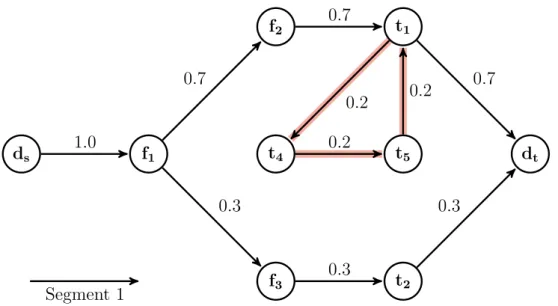
end-depot, which may not necessarily be the start-depot. Fig. 1.2 illustrates the idea

of the relocation process.

ds f1 f2 f3 f4 f5 f6 f7 f8 t1 t2 t3 dt

Figure 1.2: Example of a relocation tour where a shuttle (blue arcs) twice drops off three chauffeurs at from-zone nodes and then picks them up in the to-zones. Out of eight cars available, the chauffeurs relocate six (black arcs).

While moving cars from the from-zones to the to-zones, the chauffeurs can stop at petrol stations to refuel the cars. When the cars are refuelled during the relocation the provider economise, using one employee to carry out two tasks. This is often necessary as refuelling car-sharing cars may be not convenient for the customers. Of course, the providers could also offer rewards to the customers for refuelling the cars. However, it is doubtful if this motivates the customers to stop by a petrol station since the refuelling costs time. For this reason, we assume that the providers do the refuelling and therefore prefer to relocate cars with a lower fuel level.

The car-sharing companies’ aim is to increase the utilisation rate of the cars by adapting the distribution of the vehicles between the zones to the expected demand. For this

(17)

1.2 Scope of the thesis

purpose the providers distinguish not only between from-zones and to-zones but also between the particular to-zones. This allows them to control the distribution of

the cars which are to be relocated among the individual to-zones. Therefore, the

providers determine the expected demand for each to-zone before the relocation takes place. This prediction is then used to assign individual weights to the to-zones. The higher the expected demand for a to-zone, the higher its weight and the more cars – with respect to other to-zones – should be moved to this to-zone. The maximal number of cars that can be parked in a to-zone is limited due to restricted parking space, which varies for every to-zone.

1.2 Scope of the thesis

The relocation problem was addressed by R. Bürkle, C. Grupp, M. Kaiser and M. Knoll [Bür+14], a group of mathematics students who worked on this problem during a course in summer 2014 at the Technische Universität München (TUM), Germany. They formulated this problem as a mixed-integer linear program and were able to solve it with heuristic methods. The model uses four index-sets and therefore the number of variables is comparably high. It is apparent that this high complexity influences negatively the computational time for solving the problem, especially for big problem instances (by means of number of cars and to-zones). Hence, one could consider simpler models like planing only drop-off tours or using just one shuttle bus. On the other hand, by renouncing as many simplifications as possible, this model gives a more realistic representation of the problem.

The scope of this thesis is to develop an algorithm which solves an extension of the four-index model as fast as possible. As one can show, the relocation problem is

NP-complete. That means, there is no algorithm known by now which can solve the problem

in polynomial runtime. Consequently, one has to make use of combinatorial optimisa-tion methods. The method chosen in this thesis is the branch-and-cut algorithm which is used by almost every modern Mixed-Integer Programming (MIP) solver [FLS10]. Since these solvers have to be able to solve different types of optimisation problems, the cuts they use are typically cutting planes which can be generated independently of the problem. These cuts cannot exploit the special structure of the corresponding problem. Therefore, the aim of this thesis is to find such special cuts for the relocation problem which improve the performance of an existing branch-and-cut method. To validate the usefulness of the additional cuts as well as to asses their impact, the developed branch-and-cut algorithm has to be tested on real-life instances.

(18)

Chapter 1 One-way car-sharing

Summarising, six objectives are defined:

1. Discussion and adaptation of the four-index model.

2. Identification of useful additional cutting planes which exploit the structure of the relocation problem.

3. Implementation of the developed branch-and-cut algorithm for the relocation problem in a computer program.

4. Testing the program with real-life instances. 5. Analysis of the test results.

6. Developing of a branch-and-cut method for solving the relocation problem. We achieve these objectives as follows:

In Chapter 2 we state the Vehicle Relocation Problem (VRLPOWCS) in the One-Way Car-Sharing. Then we discuss the four-index model and show that this formulation of the VRLPOWCS is correct.

Chapter 3 presents problems which are related to the VRLPOWCS. Using these relations we prove that the VRLPOWCS is NP-complete.

After giving an introduction to the theory of branch-and-cut in Chapter 4, we present and discuss in Chapter 5 several cutting planes which we deduced from the Orienteering Problem and adapted to the VRLPOWCS. In addition, we propose separation methods for three of these cutting planes and show certain correlations between them.

Chapter 6 describes the implementation of the proposed branch-and-cut algorithm in a computer program which can solve the VRLPOWCS. In Chapter 7 we state the set-up of the tests and present the test criteria we use for evaluation. In Chapter 8 we analyse and discuss the numerical results of the tests under several perspectives.

This thesis is closed in Chapter 9 with a summary and an outlook on further research questions regarding the Vehicle Relocation Problem in the One-Way Car-Sharing.

(19)

Chapter 2 The vehicle relocation problem in the

one-way car-sharing

The informal description of the relocation process in the previous chapter shows that it is a non-trivial task to find an optimal solution to this problem. Therefore, a mathematical model is introduced to describe the so called Vehicle Relocation

Problem in the One-Way Car-Sharing (VRLPOWCS). This formulation is

based on a mixed-integer linear program (MIP) proposed by R. Bürkle, C. Grupp, M. Kaiser and M. Knoll [Bür+14]. In this chapter we first define the VRLPOWCS formally and point out special characteristics of the problem. Then we discuss the adaptations and extension we made to the four-index model for our purposes. The correctness of this formulation is showed, too. Furthermore, we prove that this formulation already implies certain constraints, among others the subtour elimination constraints. Finally, we a symmetry breaking inequality for excluding certain symmetries in the model.

2.1 Problem statement

In this section we formally introduce the VRLPOWCS. To describe this problem mathematically, the following sets and parameters are introduced:

Let V be a finite node set which is partitioned into three subsets: V = {ds, dt}⊍Vf r⊍Vto.

ds and dt describe the start-depot and the end-depot. Recall that these two depots

do not necessarily have to be the same. The from-zone nodes Vf r ⊊ V stand for

the locations of the cars parked within the from-zones which can be relocated. As mentioned before, the car-sharing provider does not want to relocate all cars parked in the from-zones. Hence, in the problem only those cars (which correspond to the from-zone nodes) appear which were selected in advance as candidates for a relocation. Every from-zone node i ∈ Vf r is associated with a non-negative utility value ui∈ Q≥0.

Vto⊊ V denotes the to-zone nodes. Every to-zone node t ∈ Vto is assigned a to-zone capacity Qt∈ N. It describes the maximal number of cars that can be moved to to-zone

t∈ Vto due to limited parking space in the to-zones. Furthermore, every to-zone t ∈ Vto

(20)

Chapter 2 The vehicle relocation problem in the one-way car-sharing

the to-zones according to the expected demand. The higher the expected demand of a to-zone, the higher its weight. Dividing the weights by the total weight, Ω = ∑t∈Vtoωt,

one obtains the relative weight ωt

Ω ∈ (0, 1] of the corresponding zone t ∈ Vto. Thus,

the relative weights allow a more demand-driven distribution by preferring distinct to-zones. This is elaborated in more detail in Section 2.2.6.

The arc set A ⊊ V × V indicates the possible journeys of the shuttles and cars between the nodes i ∈ V and j ∈ V, not the actual road network in the city. Therefore, it contains the following arcs:

• [ds, j,], ∀j ∈ Vf r,

• [i, j], ∀i ∈ Vf r, j∈ V /{ds, dt},

• [i, j], ∀i ∈ Vto, j∈ V /{ds}.

The function

ty∶ A Ð→ N0

assigns every arc [i, j] ∈ A a non-negative weight. This weight is the shuttle travel

time, ty_i,j ∶= ty([i, j]) ∀[i, j] ∈ A. Note that due to one-way streets, road works or traffic

situations the travel time from node i to j may be in general not the same as from j to

i. This justifies also the usage of a directed graph (see Definition 2.1). The maximal

shuttle working time is limited by Z ∈ N.

The set of car arcs, Acar ∶= {[i, j] ∶ i ∈ Vf r, j∈ Vto} ⊊ A includes all arcs which can

be used by the cars. For all car arcs [i, j] ∈ Acar, a second weight is assigned by the

function

tx∶ AcarÐ→ N0.

It describes the car travel time, tx

i,j∶= tx([i, j]) ∀[i, j] ∈ Acar.

These sets and functions induce the so called relocation graph.

Definition 2.1 (Relocation graph)

Let V , A, ty _{and t}x _{be defined as stated above. The weighted, directed graph G =}

(V, A, ty_{, t}x_{) is called the relocation graph.}

As mentioned in Section 1.1, a fleet of shuttle buses transports the chauffeurs. The

shuttle set K = {1, . . . , K}, K ∈ N, contains all the buses which are available. Every

shuttle k has a capacity Ck∈ N which denotes the maximal number of seats.

Each shuttle can repeat the drop-off and pick-up process at most R ∈ N times. This requires the introduction of the segment set R = {1, . . . , R}. A segment r ∈ R begins

(21)

2.1 Problem statement

and ends when a shuttle k ∈ K heads from a to-zone node i ∈ Vto to a from-zone node

j∈ Vf r. The last segment 1 ≤ rlast≤ R ends when the shuttle arrives in the end-depot.

Observe that R is an upper limit on the maximal number of segments allowed. That means, a shuttle does not have to use all segments but can return to the end-depot be-fore. Then it remains there since it is not allowed to leave the end-depot any more. It is important to choose R as small as possible since it influences the problem size. However, one cannot determine R optimally in advance since this value is part of the optimal solu-tion of the VRLPOWCS. As a consequence, one has to approximate R (see Secsolu-tion 8.5). Due to the introduction of segments one has to differentiate in which segment a node is visited. Consequently, one has to clone the graph G R times and connect the individual

segment levels (cf. Fig. 2.1). By introducing segment-nodes and segment-arcs, the

nodes V and the arcs A are distinguished by their segment level.

Definition 2.2

a) Let R = {1, . . . , R}, R ∈ N, be the set of segments. Define ˜V ∶= V × R, the set of

segment-nodes. For every subset S ⊂ V define analogously ˜S∶= S × R.

b) ˜A⊊ ˜V × ˜V, is the set of segment-arcs. It contains the following directed arcs:

(i) [(ds,1), (j, 1)], ∀j ∈ Vf r,

(ii) [(i, r), (j, r)], ∀i ∈ Vf r, j∈ V /{ds, dt}, 1 ≤ r ≤ R,

(iii) [(i, r), (j, r)], ∀i ∈ Vto, j∈ Vto∪ {dt}, 1 ≤ r ≤ R,

(iv) [(i, r), (j, r + 1)], ∀i ∈ Vto, j∈ Vf r, 1 ≤ r ≤ R − 1.

The cars cannot change the segment-level, i.e. they can be only moved in the same segment. Hence, the set ˜Acar is defined as follows:

˜

Acar∶= {[(i, r), (j, s)] ∈ ˜A∶ i ∈ Vf r, j∈ Vto, r= s}. Remark 2.3 (Equivalence classes on the segment sets)

˜

V contains R times the node set V (cf. Fig. 2.1). That is, every node i ∈ V has R

clones which differ by the segment. This induces an equivalence relation: Ψ = {((i, r), (j, s)) ∈ ˜V × ˜V ∶ i = j}.

Thus, the equivalence class [i]Ψ= {(j, r) ∈ ˜V ∶ j = i, r ∈ R} represents all segment-nodes

(i, r) ∈ ˜V. To simplify notation, node i ∈ V is in the following considered as

(22)

Analogously, one can define an equivalence relation on the set of segment-arcs ˜A:

Φ = {([(i, r), (j, s)], [(g, p), (h, q)]) ∈ ˜A× ˜A∶ i = g, j = h}.

The corresponding equivalence classes are

[[(i, j)]]_Φ= {[(g, p), (h, q)] ∈ ˜V ∶ i = g, j = h ∈ R}.

They contain all the segment-arcs which connect the same nodes on different segments. Like for the segment-nodes, arc [i, j] ∈ A represents in what follows equivalence class [[(i, j)]]_Φ.

The weight functions defined for the relocation graph have to be adapted to the segment-arcs. Since the weights do not depend on the particular levels, the functions are defined on the corresponding equivalence classes.

The weight function

˜ty _{∶ ˜}_A_{/ ∼}

ΨÐ→ N0, [i, j]Ψ↦ ty([i, j]), h

assigns to every arc in the arc equivalence class [i, j]Ψ∈ ˜A/ ∼Ψ the shuttle travel time

of the corresponding arc [i, j] ∈ A in the relocation graph. In the same way the weight function

˜tx_{∶ ˜}_A

car/ ∼ΨÐ→ N0, [i, j]Ψ↦ tx([i, j])

assigns to every car arc in the car arc equivalence class [i, j]Ψ∈ ˜Acar/ ∼Ψ the car travel

time of the corresponding arc [i, j] ∈ Acar in the relocation graph.

These sets allow to define the segment-graph which contains R clones of the relocation graph (see Fig. 2.1).

Definition 2.4 (segment-graph)

Let ˜V, ˜A, ˜ty and ˜tx be defined as stated above. The weighted, directed graph

˜

G= ( ˜V , ˜A, ˜ty, ˜tx) is called the segment-graph.

Every shuttle bus can complete a tour on the segment-graph. Such a VRLPOWCS-tour is defined as follows.

Definition 2.5 (VRLPOWCS-tour)

Let ˜G= ( ˜V , ˜A, ˜ty, ˜tx) be the segment-graph. Furthermore, let K = {1, . . . , K}, K ∈ N,

be the set of available shuttles and R = {1, . . . , R}, R ∈ N, the set of available segments.

Ck∈ N denotes the maximal seat capacity of shuttle k ∈ K, Z ∈ N the maximal shuttle

working time. A VRLPOWCS-tour Tk= (a1, . . . , am), k ∈ K, is a sequence of m ∈ N

(23)

2.1 Problem statement

Figure 2.1: Illustration of a segment-graph. Each segment in the segment-graph defines a new level of the relocation graph by cloning all nodes.

1. Every segment-node (i, r) ∈ ˜V is visited at most once.

2. The first arc starts in the start-depot and is traversed in the first segment, i.e.

a1= [(ds,1), (j, 1)] for some j ∈ Vf r.

3. The tour is connected and every segment-node entered in some arc is left in the next arc (except the start- and end-depot), i.e.

al−1= [(i, r), (j, s)] ⇒ al= [(j, r), (h, p)] for i, j, h ∈ V, 1 ≤ r ≤ s ≤ p ≤ R,

2 ≤ l ≤ m.

4. The last arc connects a to-zone node with the end-depot dt in some segment

1 ≤ r ≤ R: am= [(i, r), (dt, r)], i ∈ Vto.

5. The travel time of the tour does not exceed a given time limit Z ∈ N: ∑m

l=1

tyal≤ Z.

If shuttle ˆk is not used for a tour, the corresponding VRLPOWCS-tour is an empty sequence, Tˆ_k= ().

In the VRLPOWCS, multiple tours can be combined. Consequently, the VRLPOWCS is defined in the following way.

(24)

Definition 2.6 (Vehicle Relocation Problem in the One-Way Car-Sharing)

Given

• ˜G= ( ˜V , ˜A, ˜ty, ˜tx), the segment-graph,

• K = {1, . . . , K}, K ∈ N, the set of available shuttles, • R = {1, . . . , R}, R ∈ N, the set of available segments, • Ck∈ N, the maximal seat capacity of shuttle k ∈ K,

• Z ∈ N, the maximal shuttle working time, • Qt∈ N, the capacity of to-zone t ∈ Vto,

• ωt∈ N, the weight of to-zone t ∈ Vto,

• ui, the utility value assigned to from-zone node i ∈ Vf r,

find a set of VRLPOWCS-tours, T = (T1, . . . ,TK), such that:

1. Every from-zone node i ∈ Vf r is visited at most once.

2. The cars are relocated such that in no to-zone node t ∈ Vto the capacity limit Qt

is exceeded.

3. The relocation utility is maximised with respect to the smallest possible deviation from the distribution of the cars among the to-zones as imposed by the weights

ωt, t ∈ Vto.

Having defined the VRLPOWCS, in the next section we present a mixed-integer linear program which formulates this problem.

2.2 Mathematical modeling

In the following we show how we formulate the VRLPOWCS stated in Definition 2.6 as an mixed-integer linear program. Therefore, the index sets, parameters, variables and (in)equalities related to this optimisation problem are discussed. As previously mentioned, this model is an extension of another formulation (cf. [Bür+14]). The main amendments we did concern the objective function, the introduction of soft-constraints and the timing soft-constraints. An overview of the entire program can be found in Appendix A.

(25)

2.2 Mathematical modeling

2.2.1 Assumptions

To state a mathematical formulation of the VRLPOWCS, certain assumptions have to be made.

• It is assumed that the cars designated for relocation are “locked” for the customers. That means, the shuttles do not have to adapt their routes during the tours due to the fact that existing cars “vanish” or new ones “appear”.

• Furthermore, it is presumed that the from-zones are widely distributed whereas the parking places in the to-zones are rather clustered. This justifies the assumption that the shuttle bus drops off the chauffeurs near the particular cars in the from-zones while in the to-zones the shuttle stops only once at a predefined meeting point. The chauffeurs need therefore some transfer time to get to the from-zone cars and later to the meeting point in the to-zone. This transfer time

U ∈ N is assumed to be the same for all zones and for all chauffeurs and is added

to the travel time of the cars.

• The shuttle fleet is considered to be homogeneous, i.e. all buses have the same capacity C ∈ N: Ck= C ∀k ∈ K. In addition, it is assumed that every shuttle is

fully occupied.

• The time unit used in this model are seconds.

• The (minimal) travel times between the particular stops are computed in advance by aid of a route planner.

• The shuttle buses are presumably minibuses. Consequently, the net travel time for the cars and the buses is the same. The decision if a car has to be refuelled is also taken in advance. The time for fuelling is then already included in the travel time of the corresponding car. Thus, the travel time of the cars is in general longer as the one of the shuttles since the cars have eventually to be refuelled. • The function

u∶ Vf rÐ→ [1, 2], i ↦ 2 − fi,

defines the utility values. It depends solely on the relative fuel level of the corresponding car i ∈ Vf r, fi∈ [0, 1]. ui ∶= u(i), describes the relocation utility of

the car associated with from-zone node i ∈ Vf r.

2.2.2 Sets

The model is defined on the relocation graph G = (V, A, ty_{, t}x_{) (see Definition 2.1)}

(26)

Remark 2.7).

Vf r = {1, . . . , nf}, nf ∈ N, denotes the from-zone nodes, Vto= {1, . . . , nt}, nt∈ N, the

to-zone nodes. Sometimes it can be useful to decompose V into two other subsets,

V = Vout⊍ Vin with Vout= {ds} ∪ Vf r and Vin= Vto∪ {dt}.

The sets K and R are defined as stated in Section 2.1. That means, the number of available shuttles K (and thus of available chauffeurs), and the maximal number of segments allowed R is set in advance.

2.2.3 Parameters

Besides the parameters which are used under certain assumptions (see Section 2.2.1), the model uses the parameters as described in Section 2.1:

• Qt∈ N, capacity of to-zone t ∈ Vto.

• wt∈ N, weight of to-zone t ∈ Vto.

• Z ∈ N, maximal working time for the shuttles.

2.2.4 Variables

To formulate the optimisation problem five variables are used:

The binary variable yi,j,k,r (called shuttle decision variable) decides if shuttle k ∈ K

goes from node i ∈ V to node j ∈ V in segment r ∈ R. It is defined as

yi,j,k,r=⎧⎪⎪⎨⎪⎪

⎩

1, if shuttle k ∈ K goes from node i ∈ V to node j ∈ V in segment r ∈ R, 0, else.

Remark 2.7 (Shuttle decision variables induce a segment-graph)

The shuttle decision variables yi,j,k,r allow to distinguish which arc [i, j] ∈ A is used

in which segment r ∈ R by a shuttle k ∈ K. Hence, the shuttle decision variables define which segment-arcs [(i, r), (j, s)] ∈ ˜A are traversed by shuttle k and thus also

which segment-nodes (i, r) ∈ ˜V are visited. Consequently, the usage of these variables

induces the node set ˜Vy = ˜V and the arc set ˜Ay ⊋ ˜A. In combination with some

distinct constraints (see Section 2.2.6), this arc set ˜Ay can be restricted to ˜Ay_rest such

that ˜Ay_rest= ˜A holds. Summarising, by aid of the shuttle decision variables the

segment-graph ˜G can be induced.

Thus, it is sufficient to use the relocation graph G as framework for assigning the parameters (travel times, weights and capacities of the to-zones, relocation utilities of

(27)

the from-zones) to the nodes i ∈ V and arcs [i, j] ∈ A, which represent the equivalence classes of segment-nodes ˜V/ ∼Φ and segment-arcs ˜A/ ∼Ψ.

Analogously to the shuttle decision variable, the binary variable xi,j,k,r (car decision variable) determines if a car parked at from-zone node i ∈ Vf r is moved to to-zone

node j ∈ Vto by a chauffeur who has been dropped off by shuttle k ∈ K in segment

r∈ R: xi,j,k,r= ⎧⎪⎪⎪ ⎪⎨ ⎪⎪⎪⎪ ⎩

1, if a car is moved from i ∈ Vf r to j ∈ Vto by a chauffeur that has been

dropped off by shuttle k ∈ K in segment r ∈ R 0, else.

Due to different travel times for the shuttles and for the cars, the drop-off and the pick-up times have to be coordinated. This is done by using the timing variable

wi,k,r ∈ N. It defines the time point at which shuttle k ∈ K arrives at node i ∈ V in

segment r ∈ R and is limited by the maximal working time Z ∈ N.

The distribution of the cars among the to-zones is modelled by aid of soft-constraints (see inequalities (2.15) and (2.16)). For that purpose, two penalty variables are introduced: pt∈ [0, +∞) measures the positive deviation of the car distribution in the

corresponding to-zone t ∈ Vto, qt∈ [0, +∞) the negative deviation.

2.2.5 Objective

The Vehicle Relocation Problem in the One-Way Car-Sharing asks for a solution that maximises the utility of relocating cars from from-zones to to-zones in a given time period while taking into account some given distribution between the to-zones. Thus, both requirements – maximise the total relocation utility and distribute the cars between the to-zones according to the predefined distribution – have to be incorporated in the objective function.

To obtain the total relocation utility, one has to sum up the utility values of all cars which are relocated. This is the case when ∑j∈Vto∑k∈K∑r∈Rxi,j,k,r= 1. Consequently,

the first component of the objective function is ∑ i∈Vf r ui⋅ ( ∑ j∈Vto ∑ k∈K ∑ r∈R xi,j,k,r).

The distribution of the cars between the to-zones according to the weights is formulated in this model by aid of soft-constraints. The deviation of the actual distribution from the imposed one is therefore penalised by subtracting the penalty variables from the

(28)

total relocation utility. Hence,

− ∑

t∈Vto

(pt+ qt)

is added as the second component to the objective function. Both components are then combined in a convex combination. A trade-off parameter λ ∈ [0, 1] controls the impact of the soft-constraints (the higher lambda, the more the distribution is taken into account). Summarising, the objective function of the VRLPOWCS looks as follows: max ((1 − λ) ⋅ ∑ i∈Vf r ui⋅ ( ∑ j∈Vto ∑ k∈K ∑ r∈R xi,j,k,r) − λ ⋅ ∑ t∈Vto (pt+ qt)). (2.0) 2.2.6 Constraints

Before stating the constraints, a simplifying notation is introduced:

Notation

As mentioned above, the model is formulated on the relocation graph G = (V, A, ty_{, t}x_).

Consequently, the shuttle decision variables yi,j,k,r are only defined for arcs [i, j] ∈ A.

Thus, given two node sets V1, V2⊆ V , the sum over the shuttle decision variables has

to be of the form

∑

[i,j]∈A∶

i∈V1,j∈V2

yi,j,k,r.

Although mathematically correct, this notation is rather cumbersome. Therefore, this notation is substituted by the following one:

∑

i∈V1

∑

i∈V2

yi,j,k,r.

Strictly speaking, this notation is wrong since it includes arcs which are not defined in the relocation graph, too. However, this notation increases the readability and thus it is used in the thesis to define the sum over a set B = {[i, j] ∈ A ∶ i ∈ V1, j∈ V2}.

The constraints can be categorised into five classes: connectivity constraints, drop-off and pick-up constraints, timing constraints, to-zone constraints and variable-defining constraints.

(29)

Connectivity constraints

Setting the corresponding car decision variables to zero, it is guaranteed that the cars can be moved only to to-zones

xi,j,k,r= 0 ∀i ∈ V, j ∈ V /Vto, k∈ K, r ∈ R, (2.1)

and never again out of any to-zone

xi,j,k,r= 0 ∀i ∈ Vto, j∈ V, k ∈ K, r ∈ R. (2.2)

The outflow (of the shuttles) from the start-depot is restricted to one by ∑

j∈Vf r

yds,j,k,1≤ 1 ∀k ∈ K. (2.3)

The inequality states that the shuttles can (but do not have to) leave the start-depot. The reason for this is the fact that eventually not all K shuttles are necessary for relocating cars and therefore the provider can economise by using the minimal number of shuttles required.

As mentioned in Remark 2.7, the model is formulated on the relocation graph which contains only distinct arcs. However, in contrast to the segment-graph, the relocation graph does not distinguish the arcs by segments. Consequently, these arcs have to be excluded by setting the outflow out of the start-depot in any segment (except the first one) to zero,

yds,j,k,r= 0 ∀j ∈ Vf r, k∈ K, r ∈ R/{1}. (2.4)

Since the shuttles do not have to leave the start-depot, they should be forced to enter the end-depot only if they do a tour. Thus, the inflow to the end-depot has to equal the outflow from the start-depot

∑ i∈Vto ∑ r∈R yi,dt,k,r− ∑ j∈Vf r yds,j,k,1= 0 ∀k ∈ K. (2.5)

The flow conservation is ensured by three constraints in the model. This is also based on the fact that the shuttle decision variables induce an arc set ˜Ay which has to be

restricted to ˜Ay_rest (see Remark 2.7). The first constraint

∑

j∈V

yi,j,k,1= ∑ j∈Vout

yj,i,k,1 ∀i ∈ Vf r, k∈ K, (2.6)

states that in the first segment the outflow has to equal the inflow for any from-zone node.

(30)

By definition of a VRLPOWCS-tour, a new segment r ∈ R/{1} can be only begun by traversing an arc leading from a to-zone node to a from-zone node. Thus, the outflow for every from-zone node visited in a segment r ∈ R/{1} has to equal the inflow from any other from-zone node in the same segment r or the inflow from a to-zone node which was visited in segment r − 1, i.e. one segment before. This is formulated in the second flow conservation constraint:

∑ j∈V yi,j,k,r= ∑ j∈Vf r yj,i,k,r+ ∑ j∈Vto yj,i,k,r−1 ∀i ∈ Vf r, k∈ K, r ∈ R/{1}. (2.7)

To-zone nodes can be preceded or succeeded by any nodes except the start-depot which is already excluded by the definition of the relocation graph. Thus, it is sufficient to require for all to-zone nodes that the inflow equals the outflow.

∑

j∈V

yi,j,k,r= ∑ j∈V

yj,i,k,r ∀i ∈ Vto, k∈ K, r ∈ R. (2.8)

As mentioned before, it suffices to visit each node in a from-zone at most once since every node i ∈ Vf r represents a single car that can be moved. Hence, the total inflow

for every from-zone node j ∈ Vf r should not exceed one:

∑ i∈V ∑ k∈K ∑ r∈R yi,j,k,r≤ 1 ∀j ∈ Vf r. (2.9)

In contrary, the to-zone nodes can be visited multiple times due to the fact that several cars can be relocated to the same to-zone.

Remark 2.8 (Arc decision variables imply node decision variables)

In many models, a third binary variable, say zi,k,r, is defined to decide if node i ∈ V is

visited by shuttle k ∈ K in segment r ∈ R:

zi,k,r=⎧⎪⎪⎨⎪⎪

⎩

1, if node i ∈ V is visited by shuttle k ∈ K in segment r ∈ R 0, else.

However, the shuttle decision variables already imply zi,k,r since

zi,k,r= ∑ j∈V

yi,j,k,r ∀i ∈ V, k ∈ K, r ∈ R

and ∑j∈V yi,j,k,r≤ 1 by virtue of constraint (2.3). The car decision variables in

combi-nation with constraint (2.9) also imply zi,k,r, but only for from-zone nodes i ∈ Vf r

zi,k,r = ∑ j∈Vto

(31)

as well as to-zone nodes j ∈ Vto

zi,k,r = ∑ i∈Vf r

xi,j,k,r ∀j ∈ Vto, k∈ K, r ∈ R.

In addition, the timing variable wi,k,r ∈ N is only defined when a node i ∈ V is visited

by shuttle k ∈ K in segment r ∈ R. Consequently, it is not necessary to introduce such a node decision variable.

Drop-off and pick-up constraints

By setting the shuttle inflow equal to the car outflow at every from-zone node i ∈ Vf r,

the following constraint allows the shuttle to drop off a chauffeur only at a car which is relocated: ∑ j∈V yi,j,k,r= ∑ j∈Vto xi,j,k,r ∀i ∈ Vf r, k∈ K, r ∈ R. (2.10)

For regulating the pick-up of the chauffeurs, two inequalities are necessary. The first inequality makes sure that the shuttle picks up a chauffeur who has relocated a car to to-zone j ∈ Vto in the same segment. Therefore, the shuttle inflow has to be greater

than or equal to the value of the corresponding car decision variable:

xi,j,k,r≤ ∑ l∈V

yj,l,k,r ∀i ∈ Vf r, j∈ Vto, k∈ K, r ∈ R. (2.11)

The second inequality ensures that to-zone j ∈ Vtois only visited by a shuttle if at least

one car has been relocated to this node. This is achieved by limiting the shuttle outflow in every to-zone node by the aggregated car inflow in the corresponding to-zone node:

∑

l∈V

yj,l,k,r≤ ∑ i∈Vf r

xi,j,k,r ∀j ∈ Vto, k∈ K, r ∈ R. (2.12)

Note, (2.11) and (2.12) guarantee that a chauffeur is picked up by the same shuttle that has dropped him off. This is required due to organisational reasons (see Section 1.1).

The shuttle-fleet has a (homogeneous) maximal transportation capacity which cannot be exceeded. Consequently, every shuttle can visit in every segment at most C ∈ N from-zone nodes. That is, the total outflow in all from-zone nodes for shuttle k in segment r has to be less than or equal to the capacity C:

∑

i∈Vf r

∑

j∈V

(32)

To-zone constraints

Every to-zone has a maximal capacity Qt which must not be exceeded. Therefore, the

total number of cars that are moved to the zone (i.e. the sum over all car decision variables summed over all shuttles and all segments) is limited by Qt:

∑ i∈Vf r ∑ k∈K ∑ r∈R xi,t,k,r≤ Qt ∀t ∈ Vto. (2.14)

As mentioned before, the weights ωt of the to-zones are based on demand predictions.

Thus, some slight deviation from the given distribution (by means of number of cars) may be allowed. As a consequence, the weighted distribution is formulated as soft-constraints in this model. “Soft constraint are those [soft-constraints] we would like to be true - but not at the expense of the others.” [Uni09]. The first constraint controls the undercut of the required number of cars, i.e. that the percentage of the total number of cars, which should be relocated to this zone (determined by wt

Ω), is not significantly

higher than the actual number of cars relocated to this zone.

wt Ω ⋅ ∑i∈Vf r ∑ j∈Vto ∑ k∈K ∑ r∈R xi,j,k,r− ∑ i∈Vf r ∑ k∈K ∑ r∈R xi,t,k,r ≤ pt ∀t ∈ Vto. (2.15)

Analogously, the second constraint ensures that the distribution is not exceeded at any to-zone t ∈ Vto −wt Ω ⋅ ∑i∈Vf r ∑ j∈Vto ∑ k∈K ∑ r∈R xi,j,k,r+ ∑ i∈Vf r ∑ k∈K ∑ r∈R xi,t,k,r≤ qt ∀t ∈ Vto. (2.16)

The penalty variables pt and qt have to be at least as large as the corresponding

differences. Thus, the more a soft-constraint is violated and consequently the larger the difference, the larger is ptor qt. Since the penalty variables are negatively included in the

objective (2.0), the optimal solution will presumably resemble the desired distribution.

Timing constraints

In order to coordinate the drop-off and pick-up between the shuttle and the chauffeurs, five timing constraints are necessary. The starting time of all shuttles is set to zero

wds,k,1= 0 ∀k ∈ K. (2.17) wj,k,r, the earliest arrival time at an incoming node j ∈ V /{ds, dt} for some shuttle k in

segment r, can be modelled in the following way: wj,k,r has to be greater than or equal

to wi,k,r, the starting time at the preceding node i ∈ Vf r plus U, the transfer time of

the chauffeur, plus ty

i,j the travel time of the shuttle from node i to node j. This is of

(33)

variables do not need to be determined. Based on these considerations one obtains the following inequality:

yi,j,k,r⋅ (wi,k,r+ U + tyi,j− wj,k,r) ≤ 0 ∀i ∈ Vf r, j∈ V /{ds, dt}, k ∈ K, r ∈ R. (2.18)

As one can see, (2.18) is a non-linear inequality. Nevertheless, the inequality can be linearised with the aid of the modified big-M method [KTF09, p. 105]. By using a sufficient large constant, called big-M, it is guaranteed that no feasible solution is excluded when linearising the inequality. The smallest possible big-M for inequality (2.18) is (Z + U + ty

i,j). Consequently, introducing the term (Z + U + t y

i,j) ⋅ (1 − yi,j,k,r)

one obtains the linear drop-off timing constraint

wi,k,r+ U + ty_i,j ≤ wj,k,r+ (Z + U + ty_i,j) ⋅ (1 − yi,j,k,r) ∀i ∈ Vf r, j∈ V /{ds, dt}, (2.19)

k∈ K, r ∈ R.

The following lemma shows that the linear and the non-linear constraints are equivalent.

Lemma 2.9 (Linearised timing constraint)

Let G= (V, A, ty, tx) be the relocation graph, K the set of available shuttles, R the set of available segments. Furthermore, let the shuttle decision variables yi,j,k,r and the

timing variables w_i,k,r as well as all parameters be as stated above and constraints (2.0) - (2.17) and (2.24) - (2.28) hold. Then the linearised drop-off timing constraint (2.19)

is equivalent to the non-linear drop-off timing constraint (2.18).

Proof. Consider the two possible cases:

(i) Shuttle k drives in segment r from node i to j. Then yi,j,k,r= 1 and thus

(2.19) wi,k,r+ U + tyi,j≤ wj,k,r ⇔ wi,k,r+ U + tyi,j− wj,k,r≤ 0 (2.18).

(ii) Shuttle k does not use arc [i, j] in segment r. Then yi,j,k,r= 0 and (2.18) becomes

0 ⋅ (wi,k,r+ U + ty_i,j− wj,k,r) ≤ 0.

That means, the timing variable wj,k,r is not determined and can be freely chosen.

Inserting yi,j,k,r= 0 into (2.19) yields in

wi,k,r≤ wj,k,r+ Z ⇔ wi,k,r− Z ≤ wj,k,r.

Since wi,k,r≤ Z by constraint (2.26), the inequality above holds for arbitrary

(34)

Analogously, one models the minimum travel time for a shuttle during a pick-up (which ends after picking up the last chauffeur)

wi,k,r+ U + ty_i,j≤ wj,k,r+ (Z + U + ty_i,j) ⋅ (1 − yi,j,k,r) ∀i ∈ Vto, j∈ Vin, (2.20)

k∈ K, r ∈ R ,

for starting a new segment

wi,k,r−1+ U + ty_i,j≤ wj,k,r+ (Z + U + t_i,jy ) ⋅ (1 − yi,j,k,r) ∀i ∈ Vf r, j∈ Vto, (2.21)

k∈ K, r ∈ R/{1}

as well as the transfer time of the cars (with additional time for fuelling)

wi,k,r+ U + txi,j≤ wj,k,r+ (Z + U + txi,j) ⋅ (1 − xi,j,k,r) ∀i ∈ Vf r, j∈ Vto, (2.22)

k∈ K, r ∈ R.

At the beginning of a tour no transfer time is required. Hence, each shuttle can drive directly from the start-depot to the first from-zone node

ty_d

s,j≤ wj,k,1+ (Z + t

y

ds,j) ⋅ (1 − yds,j,k,r) ∀j ∈ Vf r, k∈ K. (2.23)

Variable-defining constraints

yi,j,k,r and xi,j,k,r are decision variables and thus binary:

yi,j,k,r∈ {0, 1} ∀i ∈ V, j ∈ V, k ∈ K, r ∈ R, (2.24)

xi,j,k,r∈ {0, 1} ∀i ∈ Vf r, j∈ Vto, k∈ K, r ∈ R. (2.25)

The timing variable wi,k,r is limited by the maximal working time

wi,k,r ≤ Z ∀i ∈ V, k ∈ K, r ∈ R. (2.26)

It is not necessary to explicitly require that wi,k,ris non-negative because this is already

implied by virtue of (2.17).

The penalty variables pt and qt have to be positive as they are subtracted in the

objective function

pt≥ 0 ∀t ∈ Vto, (2.27)

(35)

2.3 Correctness of the model

The model stated in Section 2.2 formulates the VRLPOWCS as defined in Definition 2.6 correctly. This can be shown as follows:

Implicit usage of a segment-graph

In Remark 2.7 it was already mentioned that the usage of shuttle decision variables

yi,j,k,r – defined on the relocation graph G – induces the segment-graph ˜G(see

Defini-tion 2.4). However, it was also observed that the induced arc set has to be restricted. This is ensured in the VRLPOWCS model by adding the following two constraints:

• Constraint (2.4) forbids every shuttle to use an arc leading out of the start-depot in any segment which is not the first one.

• Constraint (2.7) ensures that only arcs leading from a to-zone to a from-zone can be used for starting a new tour.

VRLPOWCS-tours

A tour that is feasible for some shuttle k to the VRLPOWCS-model (referred as

shuttle-tour) is a VRLPOWCS-tour as defined in Definition 2.5. To see this, one has

to check that a shuttle-tour fulfils the requirements of Definition 2.5.

1. The timing constraints (inequalities (2.17) and (2.19) - (2.23)) ensure that wi,k,r

is only assigned a value between 0 and Z if segment-node (i, r) is visited by shuttle k. This time point is unique (cf. Proposition 2.10). Consequently, every segment-node can be visited at most once in a shuttle-tour.

2. Constraint (2.3) states that if a shuttle is used for a tour, it has to leave the depot in the first segment in the first arc.

3. The flow conservation in the shuttle-tour is ensured by the three constraints (2.6) - (2.8). Consequently, a shuttle-tour has to be connected.

4. By virtue of constraint (2.5) and the definition of the relocation graph – no arc is leading out of the end-depot – the last arc of a shuttle-tour has to lead to the end-depot.

5. (2.26) ensures that the timing variables wi,k,rare limited by Z. Due to inequalities

(2.19) - (2.23), wi,k,r < wj,k,s holds if i is visited before j, r ≤ s (see proof of

Proposition 2.10). Consequently, a shuttle-tour cannot exceed the time limit Z. Summarising, a valid shuttle-tour is a VRLPOWCS-tour.

(36)

Feasible solution to the VRLPOWCS

A set of K shuttle-tours is a feasible solution to the VRLPOWCS (as defined in Definition 2.6), since:

1. Every from-zone node can be visited at most once by the set of shuttle-tours due to constraint (2.9).

2. Inequality (2.14) guarantees that the maximal capacity Qt of the to-zones t ∈ Vto

cannot be exceeded by the set of shuttle-tours.

3. The shuttle-tour is selected such that in the objective function (2.0) the relocation utility is maximised with respect to the distribution. The two soft-constraints (2.15) and (2.16) control the deviation of the actual distribution from the one induced by the weights wt. Any deviation is penalised in the objective function

(2.0) by using the penalty variables pt and qt defined in constraints (2.27) and

(2.28). In combination with the trade-off parameter λ, a minimisation of the deviation for the shuttle-tour set can be achieved.

The relocation utility is maximised because the model is formulated in such way that no superfluous nodes are visited. This is ensured by the definition of certain constraints.

Maximising the relocation utility

Inequalities (2.1) and (2.2) ensure that cars can be moved only from from-zone nodes to to-zone nodes in the same segment. Furthermore, a from-zone segment-node can be only visited in a shuttle-tour if there is a car located that has to be moved. This is guaranteed by constraint (2.10). By virtue of constraints (2.11) and (2.12), a to-zone segment-node is only visited in a shuttle-tour if at least one car has been moved to it in the same segment. A to-zone segment-node (j, r) ∈ ˜Vto is visited if and only if at

least one car is moved to it from a from-zone segment-node (i, r) ∈ ˜Vf r visited in the

same segment. Summarising, these constraints ensure that only those nodes are visited which help to maximise the relocation utility.

The timing constraints (2.19) - (2.23) coordinate the drop-off and pick-up process by linking the timing variable wi,k,r with the shuttle decision variable yi,j,k,r and the car

decision variable xi,j,k,r. This helps to minimise possible waiting times of the shuttles

as well as of the chauffeurs and therefore to maximise the number of nodes that can be visited by a shuttle in the limited working time Z ∈ N.

Concluding, in this section we have shown that our formulation of the VRLPOWCS is correct.

(37)

2.4 Implied inequalities

The model defined in Section 2.2 contains all constraints necessary to formulate the VRLPOWCS correctly. In particular, these inequalities (especially (2.19), (2.20) and (2.21)) imply two important inequalities: First, they ensure that every level-node is visited at most once, which is crucial for the correctness of the model. Second, the timing constraints already imply the subtour elimination constraints. These two implications are shown in the following.

2.4.1 One-off visit during a segment

The attentive reader may have noticed that constraint (2.9) allows each from-zone node i ∈ Vf r to be visited by at most one shuttle, whereas there is no similar constraint

for to-zone nodes j ∈ Vto. In fact, there is no reason to forbid multiple visits of a

to-zone nodes like in the case of from-zone nodes (see (2.9)). Nevertheless, a to-zone segment-node must not be visited twice by the same vehicle k in one segment r. This is crucial for the validity of several valid inequalities (cf. Chapter 4) as well for the correctness of the VRLPOWCS (see Section 2.4.2).

The following proposition proves that this requirement is implicitly fulfilled by using timing variables in the VRLPOWCS-model as stated in Section 2.2.

Proposition 2.10 (Unique time point)

Let G= (V, A, ty, tx) be the relocation graph, K the set of available shuttles and R the set of available segments. Given for some shuttle k ∈ K a shuttle-tour Tk which is

feasible solution to the VRLPOWCS model stated in Section 2.2. Then w_i,k,r, r∈ R, is uniquely defined for all segment-nodes (i, r) ∈ ˜V visited by shuttle k. Consequently, each segment-node is visited at most once.

Proof. Assume segment-node (i, r) ∈ ˜V is visited twice in some segment r ∈ {1, . . . , R}.

For simplification, (i, r) is distinguished such that (i1, r) ∈ ˜V denotes the segment-node

when visited for the first time, (i2, r) ∈ ˜V when visited for the second time. The

VRLPOWCS is defined on the relocation graph (see Definition 2.1) which allows no loops. Therefore, at least one other segment-node (j, r) has to be visited in between. Therefore, the following two decision variables are set to one: yi1,j,k,r = 1 and yj,i2,k,r= 1.

W.l.o.g. let i, j ∈ Vf r. By virtue of the drop-off timing constraint (2.19) this leads to

the following contradiction:

wi,k,r= wi1,k,r< wi1,k,r+ U + t

y

i1,j ≤ wj,k,r≤ wj,k,r+ U + t

y

j,i2 ≤ wi2,k,r= wi,k,r.

Thus, every segment-node can be visited at most once and its time point is uniquely

(38)

2.4.2 Subtour elimination

One of the fundamental constraints of a Vehicle Routing Problem (VRP) is the prohibition of subtours. A subtour is a disjoint cycle on a graph G = (V, A) which is not interconnected. Hence, if one does not forbid such subtours, it is possible to obtain solutions where the nodes of the graph are partitioned into several cycles, i.e. induced subgraphs. For each such a cycle there exists a VRP tour but since the cycles are not interconnected, there may not exist a VRP tour for the graph G. Such subtours can – among others – be excluded by introducing Subtour Elimination Constraints. They were initially formulated by Dantzig, Fulkerson and Johnson [DFJ54]

∑ i∈S ∑ j∈S ∑ r∈R yi,j,k,r≤ ∣S∣ − 1 ∀S ⊆ V /{ds, dt}, ∣S∣ ≥ 2, ∀ k ∈ K. (2.29)

This constraint states that inside any arbitrary set S at most ∣S∣ − 1 nodes are inter-connected. Consequently, there cannot be any cycles in S. Furthermore, as there have to be ∣S∣ arcs leading out of the ∣S∣ nodes in S, there has to be at least one arc lead-ing from a node i ∈ S to a node j ∈ V /S. That means, a tour has to leave S at least once. As discussed in the next chapter, the VRLPOWCS contains a VRP. Consequently, subtours have to be forbidden in the VRLPOWCS. This is achieved by requiring in Definition 2.5 that every segment-node is visited at most once (cf. Proposition 2.10). Nevertheless, the following corollary shows that the optimisation model defined in Section 2.2 implicitly contains the Subtour Elimination Constraint (2.29) if the decision variables yi,j,k,r and xi,j,k,r are binary. This is in general not the case when relaxing

the integrality restriction for these two variable. This fact is later used for generating cuts (cf. Section 5.1.1).

Corollary 2.11

Let G= (V, A, ty, tx) be the relocation graph, K the set of available shuttles and R the set of available segments. Recall: ˜S ⊆ ˜V is a set of segment-nodes. Given for some shuttle k ∈ K a shuttle-tour Tk which is feasible solution to the VRLPOWCS model

stated in Section 2.2. Then equations (2.19) - (2.21) imply the Subtour Elimination Constraints (2.29), i.e. ∑ i∈S ∑ j∈S ∑ r∈R yi,j,k,r≤ ∣ ˜S∣ − 1 ∀S ⊆ V /{ds, dt}, ∣S∣ ≥ 2, ∀ k ∈ K.

Proof. Let S ⊆ V /{ds, dt}, ∣S∣ ≥ 2. Consider the sum

∑ i∈S ∑ j∈S ∑ r∈R yi,j,k,r.

(39)

2.5 Symmetry breaking inequality

once. If the shuttle-tour visits not all ∣ ˜S∣ segment-nodes, nothing has to be shown.

If ∣ ˜S∣ nodes are visited, there can be at most ∣ ˜S∣ − 1 arcs leading from a segment-node

(i, r) ∈ ˜S to (j, r) ∈ ˜S. This follows from Proposition 2.10 as every segment-node can

be visited at most once and thus no cycles can be contained in ˜S. Consequently, there

can be at most ∣ ˜S∣ − 1 inner arcs in ˜S and the inequality holds. 2

2.5 Symmetry breaking inequality

At the end of this chapter, we introduce the symmetry breaking inequality (SBI). This inequality is not necessary for the correctness of the VRLPOWCS formulation. How-ever, it helps to exclude certain symmetries caused by the model.

As the shuttles are interchangeable, there exist K! permutations of every optimal solution. This may cause unnecessarily computational effort. To avoid such situations with homogeneous fleets, Coelho and Laporte suggest to introduce a symmetry breaking inequality [CL13, p. 543]: By allowing shuttle k to leave the depot only when shuttle

k− 1 also leaves the depot, some symmetry (homogeneity) of the model is “broken”.

∑

j∈Vf r

yds,j,k,1≤ ∑

j∈Vf r

yds,j,k−1,1 ∀k ∈ K/{1}.

Assume l < K shuttles leave the depot. These l shuttles are still interchangeable, i.e. there are still l! permutations possible. To break even this symmetry, one can extend the inequality. Requiring that shuttle k visits a from-zone node with a higher number than shuttle k − 1 (e.g. shuttle k − 1 visits node 5, shuttle k node 7), one obtains a one-to-one assignment of the shuttles. Thus, the symmetry breaking inequality is defined as follows. ∑ j∈Vf r j⋅ yds,j,k,1≤ ∑ j∈Vf r j⋅ yds,j,k−1,1 ∀k ∈ K/{1}. (2.30)

The usage of the symmetry breaking inequality explains also, why constraint (2.3) ∑

j∈Vf r

yds,j,k,1≤ 1 ∀k ∈ K

is formulated as inequality and not with equality. If this constraint would be set equal to one, all shuttles would have to leave the depot. This could lead to infeasible solutions in situations where l < K do a tour. If for example shuttle 5 is selected for a tour while shuttle 4 is set to stay in the start-depot, this leads to a contradiction in the symme-try breaking inequality. Consequently, one has to allow shuttles to stay in the depot. The result is that the first l shuttles are used and the other K−l will remain in the depot.

(40)

Summarising, in this chapter we defined the VRLPOWCS mathematically. To solve this problem, we proposed and discussed a mixed-integer linear program which makes use of four index sets. We showed that this model formulates the VRLPOWCS correctly. Furthermore, we justified why the formulation does not explicitly contain the subtour elimination constraints. Finally, we enhanced the model with the symmetry breaking inequality which excludes symmetries caused by the homogeneity of the shuttles.

(41)