1
Assessing the cost impact of competitive tendering in rail
infrastructure maintenance services: evidence from the Swedish
reforms (1999-2011)
Kristofer Odolinski (VTI), Andrew S.J. Smith (ITS Leeds)
CTS Working Paper 2014:17
Abstract
This is the first paper in the literature to formally study the cost impact of competitive tendering in rail maintenance. Sweden progressively opened up the market for rail maintenance services, starting in 2002. We study the cost impacts based on an unbalanced panel of contract areas between 1999 and 2011, using econometric techniques. We conclude that competitive tendering reduced costs by around 12%. This cost reduction was not associated with falling quality as measured by track quality class, track geometry or train derailments. We conclude that the gradual exposure of rail maintenance to competitive tendering in Sweden has been beneficial.
Keywords: railway, infrastructure, maintenance, tendering, contract, cost JEL Codes: H54; L92
Centre for Transport Studies SE-100 44 Stockholm
Sweden
3
1.0 Introduction
Railway systems in Europe were run as state monopolies for most of the 20th century, though these systems have been subject to major reforms since the early 1990s. The reform of the Swedish system started in 1988 with the vertical separation of train operations and rail infrastructure management; thus creating a new, separate rail infrastructure manager, the Swedish Rail Administration (Banverket). The Swedish reforms preceded the wider European reforms introduced by the European Commission aimed at revitalising Europe’s railways in 1991 (see directive (Dir. 91/440)). Rail infrastructure management was later reformed in 1998 when the production unit was separated (internally) from the administrative unit in order to create a client-contractor relationship. This reform paved the way for the decision to gradually expose the maintenance of railways to competition, a decision formally made by the Banverket board in July 2001. Hence, this reform introduced competitive tendering of maintenance contracts, where the in-house production unit competes with private firms in a public procurement. The first contract was tendered in 2002.
In April 2010 Banverket was merged with the Swedish Road Administration to form the Swedish Transport Administration (or Trafikverket); this body is now responsible for road and rail maintenance in Sweden. The governance of the contracted rail maintenance is divided between five regional units, though the planning procedures are located at a central unit responsible for all regions. As of 2012, 95 per cent of the railway network maintenance is subject to competition and six firms hold the (now) 33 contracts. The market share is concentrated among four major firms, with the former in-house production unit holding the largest share (65 per cent in 2012). The corporatisation of the in-house production came into effect in January 2010, and the company is owned by the Swedish state.
The decision to introduce competitive tendering and contracting of services offered by a state-owned monopoly is often driven by the desire to cut costs and improve quality. This is
4
achieved by the introduction of market pressure on a service previously delivered by one provider - mainly through ex-ante competition via tendering (Domberger and Jensen 1997). However, the desired outcome may not occur due to informational, transactional and administrative constraints (Laffont and Tirole 1993). Incentive schemes can be used to reduce some informational problems, but these need to be carefully designed and powered in order to avoid, for example, increases in long-run costs.
Contract design can be especially difficult for maintenance of railways, due to the interdependence between maintenance and renewals (see section 3.2). Here, the firm needs to carry out activities that will affect the performance of the infrastructure after the end of the contract period. Moreover, a high capacity usage of the tracks makes the railway system sensitive to disruptions and access to the tracks is therefore restrictive. This requires close planning and cooperation with train operators, while taking into account the relationship between certain maintenance activities and track quality and costs. Furthermore, appropriate specification and monitoring of quality is needed, which in the case of railways can vary depending on for example the type of traffic and the characteristics of the tracks.
Introducing competitive tendering therefore calls for a careful analysis of the special features of the railway system. Indeed, the first railway maintenance contracts in Sweden were awarded to the in-house production unit and the exposure to competition was gradual, which indicate that the contracts tendered first were part of a learning process for the infrastructure manager. However, no basis was constructed for how to measure delivery against the objectives of the reform and evaluate what role tendering would play in delivering improved outcomes (Trafikverket 2012).
There has been an extensive literature studying the impact of competitive tendering in the provision of passenger train operations (Alexandersson, 2009; Brenck and Peter, 2007, Smith et. al., 2009; Smith and Wheat, 2012). However, there has been little or no evidence on the
5
cost impact of competitive tendering in rail maintenance. Most research on railway maintenance costs has been concerned with estimating marginal costs for the purpose of determining cost-reflective charges for access to the infrastructure (Johansson and Nilsson, 2004; Andersson (2007; 2009); Wheat and Smith, 2008; and Wheat et. al., 2009). Whilst there exists a wide literature dealing with productivity and efficiency of railway systems (see for example McGeehan, H. 1993; Andrikopoulus and Loizedes 1998, Coelli and Perelman 1999 and 2000; Oum and Yu 1994; Oum et al. 1999), research on the cost, efficiency and productivity performance of rail infrastructure is much more limited.
Kennedy and Smith (2004) study the efficiency and productivity performance of rail maintenance in Britain over the period 1996 to 2002. However, this study did not permit a full before and after evaluation of tendering as the contract areas were already set up at the start of the first year covered by the study; and the data was at regional zone level, rather than contract area level. The paper does, however, show that whilst privatization, and the associated sub-contracting of all track maintenance on the network, led to lower costs initially, concerns over the quality of the track later led to a sharp rise in costs and ultimately Network Rail bringing track maintenance back in-house. Smith (2012) compared the efficiency performance of Network Rail (infrastructure maintenance and renewal costs) against other European railways over the period 1996 to 2006. Again, this study did not focus on changes in rail maintenance regimes and used national data. Finally, case studies of railway maintenance contracts in Sweden have been made by Espling (2007), though costs were not included. To the authors’ knowledge, therefore, the cost impact of competitive tendering in rail maintenance has not been formally tested (in Sweden or elsewhere in the world).
Our paper therefore fills an important gap in the literature and aims to measure and test statistically the cost impact of competitive tendering in rail maintenance using econometric
6
methods. Our findings are relevant not just for Sweden but to other railways across Europe and elsewhere (for example, the U.S. where very little track maintenance work is sub-contracted) considering whether tendering could be used to bring costs down without sacrificing quality. This issue is particularly important given the negative experience in Britain following contracting out of track maintenance noted earlier. We use an unbalanced panel of 39 contract areas over the period 1999 to 2011; this being a new, unique, dataset, collected specifically for the purpose of this study. Hence, this period covers the years before the first maintenance contract was tendered (tendering started in 2002 as noted) and extends to 2011, by which time the majority of the railway network had been subject to competitive tendering. We control for heterogeneity and quality, the latter being particularly important given the negative experiences of rail maintenance in Britain with respect to quality noted in the literature (and of course widely in the tendering literature).
The paper is structured as follows. After this introduction, section 2 sets out our research questions. Section 3 outlines the methodology and the data is described in section 4. The results are set out and discussed in section 5. Section 6 concludes.
2.0 Research questions
The policy of gradual exposure to competitive tendering implies that a decision had to be made regarding which contracts to tender first. According to Espling (2007), lines with low traffic intensity and technical complexity were tendered first. These contracts may therefore have had systematically lower costs compared to other areas prior to competitive tendering. If there is a systematic cost difference between areas tendered first and other areas, not captured by the explanatory variables in the model, then the inclusion of a simple tendering dummy to capture the impact of tendering could result in omitted variables bias (selection bias). In the
7
context of competitive tendering, this kind of bias is addressed by for example Domberger et al. (1987) and Smith and Wheat (2012).
Our overarching question is as follows: did competitive tendering of rail maintenance in Sweden lead to lower costs? To address the problem of selection bias we formulate four specific sub-questions as follows (these are later translated into hypotheses in section 3 below):
1. Were the costs of contract areas tendered first systematically different from other contracts, prior to competitive tendering?
2. Did competitive tendering have any effects on costs for the contract areas tendered first?
3. What effect did competitive tendering have on costs for contract areas tendered later? 4. Following competitive tendering, do the two groups of contract areas have the same
costs?
Research question 1 is important for addressing the possible selection bias. If such bias is present, then question 2 and 3 are essential for tracking the effects of competitive tendering. Asking whether costs are at the same level after competitive tendering (research question 4) for the two groups tells us whether there are any significant differences between tendered contract areas not captured by our estimated model.
3.0 Methodology
With access to data for cross-sectional units observed over 13 years, we can estimate panel data models. Following Greene (2012), the modeling framework can be expressed as:
8
where yit is the dependent variable, x’it is a vector of observed variables that can change
across i (individuals) and t (time), z’iα is the individual effect where z’i includes a constant
term and observed or unobserved variables, εit is the error term and β is the vector of
parameters to be estimated. In our case the i (individual) subscript refers to rail maintenance contract areas. When z’i is not observed and correlated with xit, the fixed effects model can be
used:
, (2)
where αi = z’iα is a contract area specific constant term. The fixed effects estimator uses
within-group variation, and can therefore not estimate the effect of time-invariant variables. If z’i is not correlated with xit, the random effects model can be estimated:
(3)
whereui is the contract area specific random effect. Efficient and consistent estimates can be
obtained using feasible generalized least squares, using an estimator that is a weighted average of the between- and within-groups estimators. An advantage of the random effects model is that time-invariant variables can be included. However, if the assumption of z’i being
uncorrelated with xit, does not hold, the random effects estimation will be inconsistent, while
the fixed estimator will be consistent irrespective (Wooldridge 2002).
3.1 Modelling approach
There might be unobserved effects across contract areas that affect maintenance costs and are correlated with infrastructure characteristics. Presence of such unobserved effects would favour the use of a fixed effects model. However, if these effects are observed through the available explanatory variables, a random effects model might be preferred. A comparison of the random and fixed effects model can be made using a test proposed by Hausman (1978), which is a test for the presence of systematic differences between the random and fixed
9
effects estimators. The result of the Hausman test is presented in section 5.1, and favours the use of the random effects estimator in our case.
We estimate a cost model using both fixed and random effects, though selecting the random effects model as our preferred approach as noted above. The cost model is represented by:
( ) (4)
where i = 1,2,…,N contract areas and t = 1,2,…,T years, Qit is a vector of variables describing
traffic volumes, Wit is a proxy for the input price (average hourly wage), Nit is a vector of
network characteristics and quality, Zit is a vector of dummy variables which includes policy
variables and year dummies and β is a vector of parameters to be estimated along with the constant α. The dependent variable Cit is maintenance costs.
Prices on the materials used in the production are assumed to be constant between contract areas because Trafikverket procures these in the main on behalf of the contract holders without any price discrimination (Trafikverket 2012). As is standard in the literature we estimate a translog model and test whether the Cobb-Douglas restriction can be rejected or not (see section 5).
3.2 Dynamics between maintenance and renewals
Renewals are not a part of the maintenance contracts. However, there is interdependence between renewals and maintenance; less maintenance will increase the need for renewals and vice versa. There might also be a forward looking behaviour where the maintenance costs are allowed to decrease in the year(s) prior to a planned major renewal, as shown by Andersson (2008). Another effect of renewals is the change in maintenance activities required after a major renewal. The performance and standard of the infrastructure is better after a renewal and the preventive maintenance might increase due to the associated stricter quality norms in
10
track geometry assigned to renewed tracks. This assignment of stricter quality norms is independent of the maximum speed allowed (Banverket 1997). Nonetheless, a renewed infrastructure should require less corrective maintenance. Hence, the total effect on maintenance costs after a major renewal is not obvious.
Adding renewal costs to the maintenance costs in the model is problematic because of the lumpy and cyclical nature of renewals. High renewals costs could then be interpreted as cost inefficiency for a contract area in a certain year, even though the need for the renewal might have been induced by a non-optimal maintenance strategy during several years prior to the renewal. Instead we test the possible dynamics between maintenance costs and renewals in contract areas using dummy variables for major renewals. The major renewals were identified using the same approach as Andersson (2008), where a major renewal (next year, in t+1) is defined as a situation where the renewal cost in t+1 is twice as large (or more) than the three-year moving average of maintenance costs during the period t-4 to t-2 (see equation 5). The lagged average is used in order to avoid problems with endogeneity. Using this approach, we can test if costs decrease prior to a major renewal. Following Andersson (2008), the dummy testing the forward looking behaviour is specified by:
{ (∑ ) (∑ ) } (5)
We have access to renewal costs in 1999-2012, which is necessary in order test a forward-looking behaviour during 1999-2011. Our second dummy variable for major renewals is specified by:
{
(∑ )
(∑ )} (6) where j=0 and 1. In year t, then, the dummy variable takes the value unity if a major renewal occurred in year t or year t-1. In this way, the impact of maintenance after a major renewal (in the current year and the following year) is captured. For example, if a major renewal is made
11
in 2001 in contract area A, this dummy variable will take the value 1 in 2001 and 2002. Due to lack of maintenance cost data, we could not test if major renewals have a more lasting effect on maintenance costs.1
3.3 Specification of tendering variables and hypothesis tests
In order to track the effects of tendering, we construct a vector of dummy variables:
(7)
The variables are not mutually exclusive because not all of them are used in the same model estimation. The dummy variables correspond to contract areas subject to competitive tendering (j = C), if tendered for the first time during 2002-2005 (j=F) and (j=L) if tendered for the first time during 2006-2010. A specific dummy indicates when there is a transition from not tendered to tendered in competition (j=M), making sure that the tendering variables only indicate a full year of tendering2 (see section 4.1). The subscript i denotes if the time period is before (i=B) the contract is tendered in competition or onwards (i=O), that is after competitive tendering. The vector Zjit also includes T-1 year dummies (j=Y).
Using the set of dummy variables specified in (7), we can address research questions 1-4 by testing the following hypotheses:
Hypothesis 1 βFB = 0; prior to tendering there is no difference in costs for areas
tendered 2002-2005 compared to the group of areas tendered 2006-2010 (before they were tendered) and areas never tendered.
Hypothesis 2 βFB – βFO = 0; there is no difference before and after tendering, for
areas tendered for the first time during 2002-2005.
1 To test a three-year effect, maintenance cost data in 1993 is required to avoid endogeneity bias when specifying a dummy variable for 1999 when there is a renewal in 1997 (see equation 6).
12 Hypothesis 3 βLO = 0; competitive tendering had no effect on costs for areas
tendered in 2006-2010.
Hypothesis 4 βFO - βLO = 0; tendering lowered costs to the same level for areas
tendered in 2002-2005 and areas tendered in 2006-2010.
For completeness we note that the omitted dummy variable captures the group of areas tendered 2006-2010 (before they were tendered) and areas never tendered.
3.4 Heterogeneity in production environment, infrastructure characteristics and quality
It is crucial to control for the production environment and the characteristics of the rail infrastructure in order to isolate the cost effect of tendering. Traffic volume is a cost driver, and variations are controlled for in the model. We also control for variation in climate, wages and infrastructure characteristics such as the length of track, age of switches, tunnels and bridges. Through the inclusion of year dummies, we control for effects that vary over time but not contract areas.
Moreover, lower costs do not necessarily mean that the cost efficiency has increased. One explanation could be that quality has been reduced. Including a variable for delays caused by the infrastructure - for example poor track quality - would be a good way to capture variations in the performance and robustness of the infrastructure. However, we were not able to include delays in this study due to lack of coherent data. In the final model a variable for track quality classification is used in order to control for variations in the track standard. The track quality classes are set according to the maximum speed allowed and are linked to quality norms in the
13
track geometry (see section 4.3). These quality norms are set as a safeguard against derailment and to provide good passenger comfort. Hence, including a track quality class variable in the model should ensure that an estimated cost reduction is not the result of a major change in the track standard. The quality class is however a rough estimate and does not measure track quality per se. For example, short segments with reduced speed do not affect the quality class of the track. We therefore analyse, as an off-model analysis, trends in track geometry measures in section 5.2. These measures are set in relation to the track quality class, indicating when deviations in the track geometry have reached a certain limit. Poor track geometry increases the deterioration and will shorten the service life of the track.
4.0 Data
The data set available is an unbalanced panel with observations at the track section level during the period 1999-2011. Data has been provided by Trafikverket, apart from the climate variables collected from the Swedish Metrological and Hydrological Institute (SMHI), and hourly wages collected from the Swedish National Mediation Office via Statistics Sweden. In order to make a comparison between different contract areas, data has been aggregated from track section level to contract area level. The data is presented in tables 1-5.
4.1 Contract areas
The contracts are normally tendered for 5 years with a possibility for an extension of up to two years. Given that the first contracts were tendered in the period 2002-2005, some contract areas have been tendered more than once. Moreover, since the tendering started there are contract areas that have been redesigned between contract periods, in which two areas are merged into one area or an area is split in two. More specifically, ten areas have been
14
redesigned into five new areas and two areas have been split, creating four new areas in our data set.
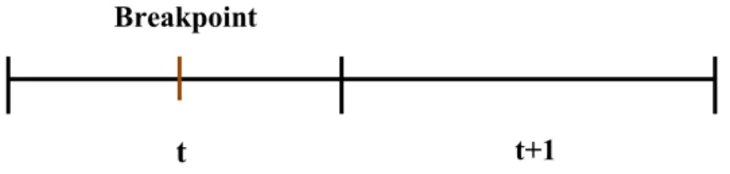
Since contract periods never start at the beginning of a calendar year, the changes in contract areas require us to create a breakpoint in the data between certain areas. The logic is visualized through figure 1, where the change occurs in year t. When the new area is formed after 30th of June (to the right of the breakpoint in figure 1) the new contract does not start until next year (t+1) in the treatment of the annual data. When the new area is formed before 1st of July (to the left of the breakpoint in figure 1), the new contract is assumed to have been in place for the whole year (t).
Figure 1 – Breakpoint in the contract period
The adjustments illustrated in Figure 1 concern 21 observations in the study. It should be noted that, as set out in section 3, we include dummy variables to capture when tendering is introduced. Hence, the forming of new areas does not affect the variables indicating when an area is subject to competitive tendering. Due to the formation of new contract areas, the data set is an unbalanced panel. In total, the data set contains 39 contract areas and 412 observations.
A case wise deletion of some track sections had to be made because of missing data. This alters the contract areas,and a limit is needed for when such alteration is too significant for a cost analysis of the contract areas. For example, economics of scale would be neglected if the size of the alteration in contract areas is ignored. We decided to use 20 per cent of the area’s
t t+1
15
total track length as the limit. Hence, a contract area is dropped from the analysis when the share of missing data exceeds this limit. Due to missing data, the study’s share of the total track length is about 80-84 per cent throughout 1999-2011. It should be noted that when areas are left in the data, but with track sections removed, both the costs and explanatory variables will be reduced.
4.2 Costs
The cost data has been retrieved from the accounting system of Trafikverket, and includes maintenance and renewals costs. In order to construct the dummy variables for major renewals (see section 3.2), we use maintenance cost data for 1994-2011, and renewal cost data for 1998-2012.
Maintenance is defined by activities conducted in order to maintain the rail network assets, and can include minor replacements. Activities included in the maintenance contracts are corrective and preventive maintenance, including snow removal. Renewals are defined as replacements or refurbishments of assets in order to return the asset to original condition (Banverket 2007).
The hourly wage data from the Swedish Mediation Office is the average gross hourly wage, SEK, for workers in the occupational category “building frame and related trade workers” in eight regions. When a contract area is located in two wage regions, an average wage is assigned to the area. We were not able to access actual wage data. One advantage of our wage measure is that it is exogenous to the infrastructure manager.
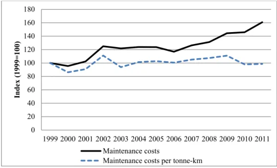
We note that maintenance costs have increased during the period 1999-2011 in our sample (figure 2). However, traffic has also increased during the same period, and the cost per tonne-km has remained broadly constant over this period.
16
Table 1 – Costs, SEK in 2012 prices*
Variable Years Obs. Mean St. Dev Min Max
Maintenance** 1994-2011 643 45 317 102 37 262 593 1 726 015 268 758 514 Renewals** 1998-2012 548 35 376 940 57 140 797 0 361 871 228
Hourly wage 1999-2011 412 154 10 129 177
*Inflation adjusted using the Swedish consumer price index, ** Does not include costs for administration and planning of maintenance/renewals
Figure 2 –Maintenance costs and unit maintenance cost indices, 2012 prices
4.3 Traffic, infrastructure characteristics and track quality
The output measures are passenger train tonnage density and freight train tonnage density, where density is defined as gross tonne-km per route-km.
Table 2 – Traffic
Variable Obs. Mean St. Dev. Min Max
Freight train tonnage density* 412 4 610 204 4 660 497 23 424 18 481 001 Passenger train tonnage density** 412 2 734 866 4 739 690 0 27 908 903
* Freight train gross tonne-km/route-km, ** Passenger train gross tonne-km/route-km
0 20 40 60 80 100 120 140 160 180 1999 2000 2001 2002 2003 2004 2005 2006 2007 2008 2009 2010 2011 Ind ex ( 19 99 = 10 0) Maintenance costs
17
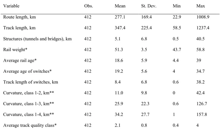
The infrastructure can be characterized by numerous variables, and the data available are shown in table 3. We have examined the correlation between infrastructure variables and find a high correlation coefficient between the curvature classes and the track length variable. All infrastructure variables are not included in the final models due to multicollinearity problems.
Table 3 - Infrastructure characteristics
Variable Obs. Mean St. Dev. Min Max
Route length, km 412 277.1 169.4 22.9 1008.9
Track length, km 412 347.4 225.4 58.5 1237.4
Structures (tunnels and bridges), km 412 5.1 6.8 0.5 40.5
Rail weight* 412 51.3 3.5 43.7 58.8
Average rail age* 412 18.6 5.9 4.4 39
Average age of switches* 412 19.2 5.6 4 34.7
Track length of switches, km 412 8.4 6.8 0.6 38.2 Curvature, class 1-2, km** 412 11.0 9.8 0 42.4 Curvature, class 1-3, km** 412 25.9 22.3 0.6 126.7 Curvature, class 1-4, km** 412 34.2 27.7 1 157.8 Average track quality class* 412 2.1 0.8 0.4 4
*Weighted mean, ** class 1: curve radius 0-300 m, class 2: curve radius 301-450 m, class 3: curve radius 451-600 m, class 4: curve radius 601-800 m
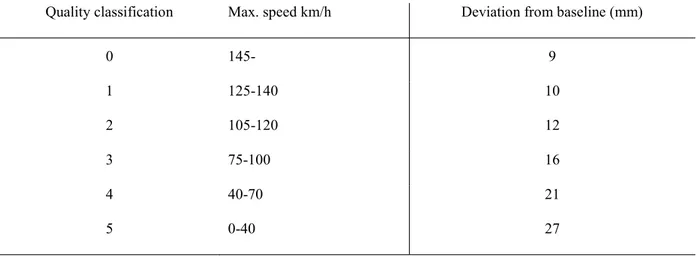
The track quality class is a number assigned to segments of track sections and is mainly decided with respect to maximum speed allowed.3 A low number on the track quality classification is given to track segments with high speed allowed and vice versa, with numbers ranging from zero to five. The expected sign of the class number in the cost analysis
3 In some cases, if the number of gross tonnes per year is under two million, a higher track class can be assigned compared to what the maximum speed allowed implies.
18
is not obvious. High speeds (a low track quality classification number) will cause a higher deterioration rate and will require more maintenance compared to tracks with low speeds (a high track quality class number), because speed is directly connected to the running dynamics of the vehicle and the track forces. Higher speed track will also need to be maintained to a higher standard. On the other hand, a high speed track will be installed to a higher standard and thus may require less maintenance as a result.
Deviations from the quality norms are measured by a track geometry car and are classified as C-errors when they reach certain limits. The limits are set according to the maximum speed allowed, that is the track quality class. A track with high speeds will have stricter limits on the deviations and vice versa (an example is presented in table 4). According to a provision by Banverket (1997), deviations in track geometry reaching the limit for C-error are defined as urgent and should be fixed immediately.
Table 4 – C-error limits on deviations in track geometry, longitudinal level
Source: Banverket (1997)
We obtained data on C-errors for the period 2002-2012 from Trafikverket. However, this variable is not included in the estimated models because the data does not cover all track sections included in the contract areas (and in any case does not extend to the period before tendering). In total, the C-error data is collected from measurements on 131 track sections,
Quality classification Max. speed km/h Deviation from baseline (mm)
0 145- 9 1 125-140 10 2 105-120 12 3 75-100 16 4 40-70 21 5 0-40 27
19
which can be compared to the 160-192 track sections included in the model. However, we separate the analysis of the trend in track geometry quality, with respect to C-errors, as an off-model analysis (see section 5.2).
4.4 Weather data
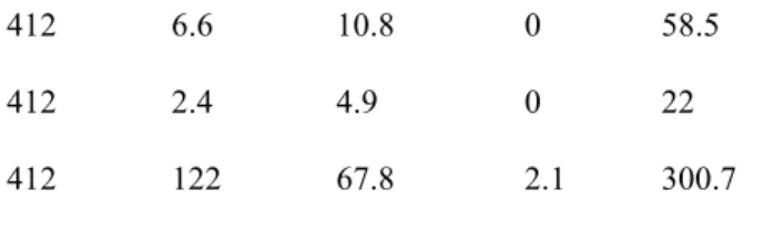
Sweden’s climate changes considerably when going from south to north. Maintenance is therefore performed in different environments. In order to account for the climate variations we have collected data on daily mean temperatures and precipitation (mm of liquid water). Data were retrieved from SMHI and consists of a time series of temperature and precipitation data at the resolution 4x4 km, which means it provides a mean value for an area over 4x4km for each day. Track sections were allocated to a 4x4 km grid, though in most cases longer sections cross over more than one grid. The temperature variable created for each track section is defined as the number of days with a temperature below a certain limit. A variable accounting for the amount of snowfall during each year was created using mm of precipitation when temperature is below zero degrees Celsius. The average values for contract areas are weighted based on the length of each track section included in the contract area. Different thresholds for temperatures are given in table 5. Due to a high correlation coefficient between temperatures and mm precipitation below zero degrees Celsius, both types of variables are not included in the estimated model.
Table 5 - Weather data
Variable Obs. Mean St. dev. Min Max
Temp. < 0 C◦*,** 412 87.8 39.6 13 185.7
Temp. < - 1 C◦*,** 412 74.6 39 8 177
Temp. < - 4 C◦*,** 412 44.9 34.7 0 142.8
20
Temp. < - 15 C◦*,** 412 6.6 10.8 0 58.5
Temp. < - 20 C◦*,** 412 2.4 4.9 0 22
Mm precipitation per year when temp. < 0 C◦ ** 412 122 67.8 2.1 300.7
* Number of days per year with temperatures below limit, **Weighted average
5.0 Results
Two models are estimated. A direct approach is used in model 1, with a dummy variable indicating when areas are subject to competitive tendering. Model 2 considers the potential selection bias arising when systematic cost differences prior to competitive tendering are not explained by the independent variables. All estimations are carried out using Stata 12 (StataCorp.11).
5.1 Econometric results
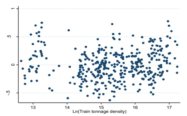
Table 6 shows the results from the model estimations. We plot the residuals and train tonnage density, which indicate the presence of heteroskedasticity (see figure 4 in appendix), though not to a substantial degree. We estimate the models using the random effects estimator and use robust standard errors. The models are also estimated using fixed effects. The results from the fixed effects estimations are presented in table 9 in the appendix, showing that the conclusions from our policy variables are robust. As Table 7 shows, the Hausman test indicates that we may adopt the random effects model as our preferred model.
Note that, in contrast to the 412 available observations, 398 observations are used in the estimations since there are observations with no passenger train tonnage, which are areas dedicated to freight traffic. With a logarithmic transformation we lose these observations in
21
the estimations. The preferred model is a double-log specification; we also estimated a translog model but could not reject the Cobb-Douglas restriction4.
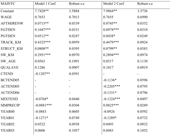
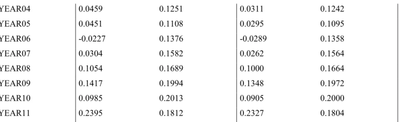
Before turning to study the impact of competitive tendering on costs, we first comment on the other parameter estimates in Table 6 (we focus on model 1 but the results are very similar between models 1 and 2). The year dummies represent effects on costs varying over time and not contract areas, with 1999 as a reference year. The dummy variables for 2000-2011 are jointly significant in the estimations, but are not individually significant and therefore do not reveal a clear trend.
Table 6 – Results
MAINTC Model 1 Coef. Robust s.e Model 2 Coef. Robust s.e
Constant 7.7428** 3.5884 7.9864** 3.5736 WAGE 0.7653 0.7013 0.7655 0.6990 AFTMJRENW 0.0715** 0.0339 0.0745** 0.0352 FGTDEN 0.1047*** 0.0331 0.0978*** 0.0310 PGTDEN 0.0512** 0.0247 0.0438* 0.0249 TRACK_KM 0.4325*** 0.0959 0.4479*** 0.0924 STRUCT_KM 0.0808** 0.0395 0.0799** 0.0383 SW_KM 0.2951*** 0.0970 0.2894*** 0.0974 SW_AGE 0.0563 0.1091 0.0517 0.1130 QUALAVE 0.1286 0.0907 0.1017 0.0919 CTEND -0.1207** 0.0591 - - BCTEND05 - - -0.1136* 0.0596 ACTEND05 - - -0.2205*** 0.0795 ACTEND06 - - -0.1331* 0.0796 MIXTEND -0.0768* 0.0440 -0.1324*** 0.0497 MMPRECIP -0.0881*** 0.0304 0.0825*** 0.0289 YEAR00 -0.0883 0.0605 -0.0926 0.0592 YEAR01 -0.1271* 0.0749 -0.1289* 0.0732 YEAR02 0.0522 0.0938 0.0493 0.0932 YEAR03 0.0606 0.1057 0.0483 0.1052
4 Our translog model included the passenger and freight output as well as network length in the translog expansion. The wage rate was not included since the addition of these extra terms did not improve the model. The results of interest on the tendering dummies appeared robust to different specifications (translog versus Cobb-Douglas and fixed versus random effects).
22 YEAR04 0.0459 0.1251 0.0311 0.1242 YEAR05 0.0451 0.1108 0.0295 0.1095 YEAR06 -0.0227 0.1376 -0.0289 0.1358 YEAR07 0.0304 0.1582 0.0262 0.1564 YEAR08 0.1054 0.1689 0.1000 0.1664 YEAR09 0.1417 0.1994 0.1348 0.1972 YEAR10 0.0985 0.2013 0.0905 0.2000 YEAR11 0.2395 0.1812 0.2327 0.1804
Note: ***, **, *: Significance at 1%, 5%, 10% level Number of observations = 398
Definition of variables in table 6:
WAGE = ln (Average gross hourly wage)
AFTMAJRENW = Dummy indicating when major renewal in year t and one year afterwards (see equation 6) FGTDEN = ln (Freight train tonnage density)
PGTDEN = ln (Passenger train tonnage density) TRACK_KM = ln (Track length)
STRUCT_KM = ln (Track length of structures (tunnels and bridges)) SW_TL = ln (Track length of switches)
SW_AGE = ln (Average age of switches)
QUALAVE = ln (Average quality class); note a high value of average quality class implies a low speed line CTEND = Dummy for years when tendered in competition
BCTEND055 = Dummy for years prior to tendering, areas tendered 2002-2005
ACTEND05 = Dummy for years when tendered in competition, areas tendered 2002-2005 ACTEND06 = Dummy for years when tendered in competition, areas tendered 2006-2010
MIXTEND = Dummy for years when mix between tendered and not tendered in competition, which is the year when tendering starts
MMPRECIP = ln (Average mm of precipitation (liquid water) when temperature < 0˚Celcius) YEAR00-YEAR11= Year dummy variables, 2000-2011
Table 7 – Diagnostic tests
Diagnosis test Model 1 Model 2
Wald test, linear restrictions of year dummies Chi2(12)=82.28, P=0.000 Chi2(12)= 80.18, P=0.000 Breusch-Pagan LM-test for Random effects Chi2(1)=341.73, P=0.000 Chi2(1)=328.48, P=0.000 Hausman’s test statistic6,7 Chi2(12)=14.92, P=0.246 Chi2(27)=15.08, P=0.373
5 Note the omitted dummy variable covers the group of areas tendered in the period 2006-2010 but for the years before they were tendered plus those areas never tendered.
6 Covariance matrixes based on disturbance estimate obtained from the random effects estimator 7 Year dummies are excluded in the test (see Imbens and Wooldridge 2007)
23
The estimates on freight traffic, FGTDEN, show an elasticity of 0.10, while the elasticity for passenger traffic, PGTDEN, is 0.05. Thus, the estimated usage elasticity, which is the elasticity of maintenance cost with respect to traffic, is quite low compared to the elasticities from previous estimations on Swedish data (see Andersson 2008) and the elasticities estimated for a number of European countries (including Sweden), which lies in the interval 0.20-0.35 (Wheat et al. 2009). That said, one study reported in Wheat et al. 2009 did have a usage elasticity of 0.18 which is similar to the sum of the passenger and freight elasticities reported here. The parameter estimates on network characteristics have the expected signs and are statistically significant, except average switch age, SW_AGE. The track quality class coefficient, QUALAVE, is not statistically significant, which might reflect the opposing effects of high (low) line speeds, which require high (low) track standards. High (low) speeds increase (decrease) the deterioration rate of the tracks ceteris paribus, while high (low) track standards decrease (increase) the deterioration rate, ceteris paribus.
The sum of the parameter estimates for track length, switch length and length of structures is smaller than one (0.8084), and a hypothesis test of constant returns to scale can be rejected at the 1 per cent level. Hence, we have an indication of increasing returns to scale.
The coefficient for wage is not significant, which might indicate that the proxy for wages does not reflect real differences in wage costs between areas. One explanation is that wages are still rather constant between different areas, an assumption suggested by Johansson and Nilsson (2004) and also assumed by Andersson (2009).
Different variables for weather have been tested in the model estimations, and the variable for mm of precipitation during temperatures below zero degrees Celsius, MMPERCIP, is retained in the model. The estimates show an increase in maintenance costs (the coefficient is 0.0881with p-value 0.004), which most likely is due to increased snow removal costs.
24
The dummy variable testing a forward looking behaviour in the dynamics between maintenance and major renewals, BMAJRENW, is not significant in our model estimations. However, the results show a 7.4 per cent8 increase in maintenance costs when a major renewal takes place (either in the current year or the previous year; the coefficient is 0.0715 with p-value 0.035). As noted in section 3.2, a renewed track is subject to stricter quality norms in track geometry, irrespective of the maximum speed allowed. This implies that more maintenance is required in order to retain the high track quality. The correlation between the major renewal dummy variables is 0.34 and the variable testing a forward looking behaviour is dropped from the model estimation.
Turning to the policy variables in the models, the tendering variable in model 1 shows that competitive tendering has lowered costs. The coefficient (-0.1207 with p-value = 0.041) translates into an 11.4 per cent9 decrease in maintenance costs due to tendering. The 95 per cent confidence interval [-0.2365, -0.0050] therefore shows that tendering most likely decreased costs according to model 1.
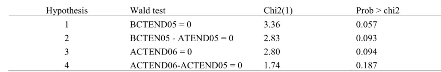
In our second model we consider the issue of possible selection bias and address the results from the hypothesis tests specified in section 3.3 (see table 8 for the results from the Wald tests of the hypotheses). The first areas tendered in competition were chosen with respect to their low traffic intensity and technical complexity so there is a prior reason to expect a possible selection bias. The first point to note is that prior to tendering the cost level for areas tendered first is not significantly different from the control group / omitted dummy at the 5 per cent level (which represents the group of areas tendered later, between 2006-2010, but during the years before they were tendered, and areas never tendered); this is hypothesis 1. However, the point estimate of -0.1136 is significant at the 10 per cent level (P-value=0.057). We further find that, post tendering, the areas tendered first are clearly cheaper than the
8 EXP(0.0715) - 1= 0.0741
25
control group (by 19.8 per cent10; P-value=0.006); and that the difference in costs before and after tendering for this group of areas is statistically significant at the 10 per cent level (hypothesis 2; P-value= 0.093).
Turning to the group of areas tendered later (in 2006-2010), the results from model 2 show that competitive tendering has lowered costs for these areas by 12.5 per cent11 (rejection of
hypothesis 3). The coefficient is -0.1331 with P-value = 0.094, with a 95 per cent confidence
interval of [-0.2890, 0.0229]. Finally, the Wald test for hypothesis 4 reveals that, following competitive tendering, there is no significant difference in costs between areas tendered first and areas tendered later (Chi2(1) = 1.74 with P-value = 0.1874). The policy results from model 2 are depicted in figure 3, which also show the 90 per cent confidence intervals for the tendering coefficients.
Table 8 – Results from hypothesis tests
Hypothesis Wald test Chi2(1) Prob > chi2
1 BCTEND05 = 0 3.36 0.057
2 BCTEN05 - ATEND05 = 0 2.83 0.093
3 ACTEND06 = 0 2.80 0.094
4 ACTEND06-ACTEND05 = 0 1.74 0.187
Overall, our results show that competitive tendering has reduced costs. In model 1 we find that the effect is a cost reduction of 11.4 per cent, and we can reject hypothesis 1 at the 5 per cent level of significance, thus indicating that the model does not suffer from selection bias. The results of our more nuanced approach in model 2 can be summarised as follows. We find that the magnitude of the coefficients for contracts tendered first is quite different (before tendering -0.1136; versus after tendering, -0.2205) and therefore points to a cost reduction from competitive tendering of 9 per cent (statistically significant at the 10 per cent level).
10 EXP(-0.2205) - 1 = -0.1978
26
Further, the costs of these areas, post-tendering, are clearly lower than the control group. Hence, we cannot rule out the possibility of a selection bias in model 1. Nevertheless, competitive tendering lowered costs by 12.5 per cent for areas tendered for the first time in 2006-2010 (significant at the 10 per cent level), which is similar to the model 1 results. Thus, the main result of the paper does not change when controlling for a possible selection bias. It is further reassuring that, post-tendering there is no statistically significant difference in the cost levels of the two types of areas, which seems to indicate that competitive pressure through tendering has brought costs down to more efficient levels. Moreover, a sensitivity analysis was made for contracts that belong to the group of contracts tendered first. More specifically, we tested if a selection bias was present when changing the definition of this group of contracts with respect to when tendering took place. No selection bias was found. This finding also provides further evidence against the hypothesis that the first group of areas has systematically lower costs than other areas for reasons not explained by the model.
27
Figure 3 – Mean cost level of areas tendered in competition – with 90 % confidence intervals - relative to baseline
5.2 Track quality
A common problem with cost studies is that cost savings can be observed if firms decide to cut quality measures; indeed private firms, and indeed public ones, may have an incentive to seek to achieve cost reduction targets through reducing quality rather than seeking genuine productivity or efficiency savings – particularly if those quality measures may go unnoticed.
In our study, if costs have decreased at the expense of track quality measures not captured by the model, we cannot necessarily conclude that cost efficiency has increased. As described in section 3.4, the quality class variable included in the model should ensure that cost reductions associated with major changes in track standard (primarily driven by maximum linespeed) are controlled for. However, it does not directly control for track quality. We
0,6 0,7 0,8 0,9 1 1,1 1,2 1,3 1,4 Mea n cost l eve l re lative to base li ne Baseline
Areas tendered for the first time 2002-2005 Areas tendered for the first time 2006-2010
Tendering starts (first full year of tendering)
28
therefore analyse trends in available measures that reflect track quality. No conclusions can be made with respect to how competitive tendering has affected these trends. Still, they show if there has been a significant change in track quality during a period in which far reaching organisational reforms have been made. We did not have sufficient observations to include this variable directly in the model.
C-errors are deviations from the ideal track geometry that have reached certain limits. Large deviations will increase the track deterioration if speed is not reduced, which shortens the service life of the tracks. The analysed data only include errors at rail lines and not stations, due to missing data. We restrict the analysis to track sections measured at least once every year by the track geometry car12. As noted earlier, this leaves us with 131 track sections out of the 160-192 included in our model estimations. We have filtered out C-errors measured more than once per year to avoid double counting. The track quality trends, measured through deviations in track geometry, show no indication of a deterioration in track quality at the aggregate network level over the period 2002-2012, rather the opposite (see figure 4).
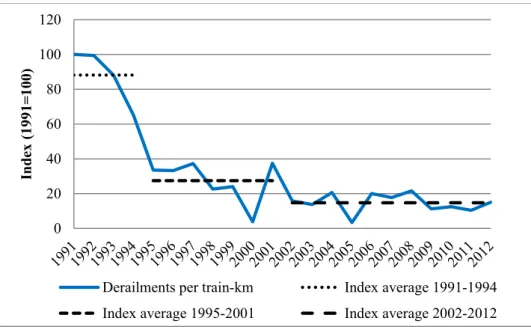
Moreover, the number of derailments per year on the Swedish railway network has decreased over the period 1991-2012 (see figure 5), while the number of train-km have increased steadily, with about 45 per cent more train-km in 2012 compared to 1991. Note that in addition to poor track quality, human error and vehicle errors cause derailments, and we do not have access to the share of derailments in figure 5 that are caused by poor track quality.
There is therefore no sign of a deteriorating track quality according to the available measures during the period of competitive tendering (though, one should be aware of a possible lag in the effect maintenance activities can have on these measures and that quality improvements in the off-model analysis can be due to renewals). Thus, on balance, we consider that competitive tendering has resulted in lower costs without negatively impacting
12 Track geometry car STRIX
29
on quality. Thus we consider that competitive tendering has improved cost efficiency in this sample.
Figure 4 –Number and track length of C-errors, 2002-2012
Figure 5 - Derailments of trains in motion per train-km, 1991-2012. Source:
Transport Analysis and the Swedish Transport Agency (Swedish government
agencies) 0 20 40 60 80 100 120 2002 2003 2004 2005 2006 2007 2008 2009 2010 2011 2012 Ind ex ( 20 02 = 10 0)
Nr. of C-errors Track length of C-errors
0 20 40 60 80 100 120 Ind ex ( 19 91 = 10 0)
Derailments per train-km Index average 1991-1994 Index average 1995-2001 Index average 2002-2012
30
6.0 Conclusion
The contribution of this paper is that it is the first to formally study the cost impact of competitive tendering in rail maintenance using econometric methods. Competitive tendering in Sweden was implemented gradually, progressively opening up in-house units around the network to competition, with the first new contract starting in 2002. We find that competitive tendering reduced costs by around 12 per cent; although, there remains some ambiguity over the precise cost impact for the first group of contracts chosen for competitive tendering.
Importantly, our model controls for differences in the production environment and infrastructure characteristics, as well as track quality class (which mainly reflects maximum linespeed). As a further, off-model analysis, we found that quality measures excluded from our model, namely track geometry and derailments, improved substantially over the tendering period. Thus, the notion that cost reductions may have been achieved by cutting quality (in the way measured here), which might be seen as a particular incentive for private firms, is firmly rejected; indeed cost reductions were achieved at the same time as quality improvements (though it must be borne in mind that there may be lags between changes in maintenance activities and these quality measures, and that renewals may have had an effect on quality). Overall then, the results show that the gradual exposure to competitive tendering has been successful.
Our findings are relevant not just for Sweden but to other railways across Europe and elsewhere considering whether tendering of rail maintenance could be used to bring costs down without sacrificing quality. This question is particularly relevant given the negative experiences of rail maintenance in Britain, noted in the previous literature, where short-term cost reductions were achieved at the expense of quality, and costs subsequently had to rise very substantially to deal with the problem (though there were other reasons for the later cost increases; see for example, Smith, 2012). Thus the evidence in this paper should provide
31
recent, positive evidence in support of competitive tendering in rail maintenance, to counter the very high profile and negative experience in the British case. A notable difference in Sweden is that tendering was introduced gradually, as compared to the “Big Bang” approach adopted in Britain. The gradual reform of track maintenance helped the infrastructure manager to keep competence within the organization, which is important when contracting out. A client that loses competence might face a higher level of information asymmetry in the client-contractor relationship, leading to adverse selection.
Our results are in line with the wider literature on competitive tendering, for example in the provision of passenger rail services and also in other industries, which has generally shown that tendering reduces costs and improves efficiency. Certainly, the literature shows that the ability of the contracting body to specify and monitor quality adequately is a critical success factor. In the Swedish context, at least based on the evidence to date, it appears that quality specification and monitoring has not been a problem; indeed, the evidence shows that it has been possible to reduce costs and increase quality simultaneously.
Future research could aim at a more in depth review of the track maintenance contracts to study how the design of contracts affects quality and costs. There is heterogeneity in the type of incentive schemes used and to what extent the payments are fixed, which is promising for a future analysis of best practice.
References
Alexandersson, G., and S. Hultén (2007): ‘Competitive Tendering of Regional and Interregional Rail Services in Sweden’, In European Conference of Ministers of Transport
Competitive Tendering of Rail Services, OECD 2007.
Alexandersson, G. (2009): ‘Rail Privatisation and Competitive Tendering in Europe’, Built
32
Andrikopoulos, A.A., and J. Loizedes (1998): ‘Cost Structure and Productivity Growth in European Railway Systems’, Applied Economics, 30(12), 1625-1639.
Andersson, M. (2007): ‘Fixed Effects Estimation of Marginal Railway Infrastructure Costs in Sweden’, Working paper 2007:11, VTI, Sweden.
Andersson, M. (2008): ‘Marginal Railway Infrastructure Costs in a Dynamic Context’, The
European Journal of Transport and Infrastructure Research (EJTIR), 8(4), 268-286.
Andersson, M. (2009): ‘Deliverable 8 - Rail Cost Allocations for Europe – Annex 1A - Marginal Cost of Railway Infrastructure Wear and Tear for Freight and Passenger Trains in Sweden’, CATRIN (Cost Allocation of TRansport INfrastructure cost).
Andersson, M., A.S.J., Smith, Å. Wikberg, and P. Wheat (2012): ‘Estimating the Marginal Cost of Railway Track Renewals Using Corner Solution Models’, Transportation
Research Part A, 46(6), 954-964.
Andersson, M., and G. Björklund (2012): ’Marginal Railway Track Renewal Costs: A survival data approach’, CTS Working Paper 2012:29, Centre for Transport Studies, Stockholm.
Asmild, M., T. Holvad, J.L. Hougaard, D., and Kronborg (2009): ’Railway Reforms: do they influence operating efficiency?’, Transportation, 36(5), 617-638.
Banverket (1997): ‘Spårlägeskontroll och kvalitetsnormer – Central mätvagn Strix’, Föreskrift BVF 587.02, (in Swedish).
Banverket (2000): ’Banområdets organisation och uppgifter’, Handbok BVH 001.4. (in Swedish).
Banverket (2007): ’Åtgärder i järnvägsnätet. Huvudprocessen utveckla och underhålla anläggning’, Standard BVS 803, (in Swedish).
33
Brenck, A., and B. Peter (2007): ‘Experience With Competitive Tendering in Germany’, In
European Conference of Ministers of Transport Competitive Tendering of Rail Services,
OECD 2007.
Cantos, P., J.M., Pastor, and L. Serrano (2012): ‘Evaluating European Railway Deregulation Using Different Approaches’, Transport Policy, 24, 67-72.
Coelli, T.J, and S. Perelman (1999): ‘A Comparison of Parametric and Non-parametric Distance Functions: With application to European railways’, European Journal of
Operational Research, 117(2), 326-339.
Coelli, T.J, and S. Perelman (2000): ‘Technical Efficiency of European Railways: a distance function approach’, Applied economics, 32(15), 1967-1976.
Domberger, S., S. Meadowcroft, and D. Thompson (1987): ‘The Impact of Competitive Tendering on the Costs of Hospital Domestic Services’, Fiscal Studies, 8(4), 39-54.
Domberger, S., and P. Jensen (1997): ‘Contracting Out by the Public Sector: theory, evidence, prospects’, Oxford Review of Economic Policy, 13(4), 67-78
Driessen, G., M. Lijesen, and M. Mulder (2006): ‘The Impact of Competition on Productive Efficiency in European Railways’, CPB Discussion paper, Netherlands Bureau for Economic Policy Analysis, No. 71.
Espling, U. (2007): ‘Maintenance Strategy for a Railway Infrastructure in a Regulated Environment’, Doctoral thesis, Luleå University of Technology, Division of operation and maintenance engineering, Luleå Railway Research Center.
Friebel, G., M. Ivaldi, and C. Vibes (2010): ‘Railway (De)Regulation: A European Efficiency comparison’, Economica, 77(305), 77-91.
Greene, W.H. (2012): ‘Econometric Analysis, 7th edition’, Prentice-Hall.
Hausman, J. A. (1978): ‘Specification Tests in Econometrics’, Econometrica, 46(6), 1251-1271.
34
Imbens, G., and J. Wooldridge (2007): ‘What’s new in Econometrics?’, The National Bureau of Economic Research (NBER) Summer Institute 2007. Lecture notes 2:
http://www.nber.org/WNE/WNEnotes.pdf (Retrieved 2014-09-01)
Johansson, P., and J-E. Nilsson (2004): ‘An Economic Analysis of Track Maintenance Costs’,
Transport Policy, 11(3), 277-286.
Kennedy, J. and A.S.J. Smith (2004): ‘Assessing the Efficient Cost of Sustaining Britain’s Rail Network. Perspectives based on zonal Comparisons’, Journal of Transport
Economics and Policy, 38(2), 157-190.
Laffont, J.-J., and J. Tirole (1993): ‘A Theory of Incentives in Procurement and Regulation’, The MIT Press, Cambridge, Massachusetts
McGeehan, H. (1993): ‘Railway Costs and Productivity Growth’, Journal of Transport
Economics and Policy, 27(1), 19-32.
Oum, T.H., and C. Yu (1994): ‘Economic Efficiency of Railways and Implications for Public Policy. A Comparative Study of the OECD Countries’ Railways’, Journal of Transport
Economics and Policy, 28(2), 121-138
Oum, T.H., W.G. Waters, and C. Yu (1999): ‘A Survey of Productivity and Efficiency Measurement in Rail Transport’, Journal of Transport Economics and Policy, 33(1), 9-42. Pollitt, M.G., and A.S.J. Smith (2002): ‘The Restructuring and Privatisation of British Rail:
Was it really that bad?’, Fiscal Studies, 23(4), 463-502.
Smith, A.S.J. (2006): ‘Are Britain’s Railways Costing Too Much? Perspectives based on TFP comparisons with British rail 1963-2002’, Journal of Transport Economics and Policy, 40(1), 1-44.
Smith, A.S.J. (2012): ‘The Application of Stochastic Frontier Panel Models in Economic Regulation: Experience from the European rail sector’, Transportation Research Part E, 48(2), 503-515.
35
Smith, A., C.A. Nash, and P. Wheat (2009): ‘Passenger rail franchising in Britain: has it been a success?’, International Journal of Transport Economics, 36 (1), 33-62.
Smith, A.S.J., and P. Wheat (2012): ‘Evaluating Alternative Policy Responses to Franchise Failure. Evidence from the passenger rail sector in Britain’, Journal of Transport
Economics and Policy, 46(1), 25-49.
StataCorp.2011: Stata Statistical Software: Release 12. College Station, TX: StataCorp LP Trafikverket (2012): ’Organisering av underhåll av den svenska järnvägsinfrastrukturen’, Dnr:
TRV2012/63556, (in Swedish).
Wheat, P., A.S.J. Smith, and C. Nash (2009): ‘Deliverable 8 - Rail Cost Allocations for Europe’, CATRIN (Cost Allocation of TRransport INfrastructure cost).
Wooldridge, J.M., (2002): ‘Econometric Analysis of Cross Section and Panel Data’, The MIT press, Cambridge, Massachusetts, London, England.
Appendix
Figure 6 – Scatterplot of residuals and train tonnage density
-.5 0 .5 1 R esid ua ls ui +e it 13 14 15 16 17
36
Table 9 - Results from the fixed effects estimations
MAINTC Model 1 Coef. Robust s.e Model 2 Coef. Robust s.e
Constant 8.5871** 3.2724 9.1075*** 3.2727 WAGE 0.7333 0.6851 0.6654 0.6944 AFTMJRENW 0.0789** 0.0352 0.0826** 0.0358 FGTDEN 0.1373** 0.0685 0.1447** 0.0701 PGTDEN -0.0378 0.0395 -0.0440 0.0404 TRACK_KM 0.4018 0.2484 0.3960 0.2445 STRUCT_KM 0.0296 0.0750 0.0350 0.0694 SW_KM 0.3592** 0.1459 0.3372** 0.1488 SW_AGE 0.1745 0.1232 0.1476 0.1341 QUALAVE -0.0587 0.2010 -0.0596 0.2053 CTEND -0.1188** 0.0571 - - BCTEND05 - - -0.1350* 0.0767 ACTEND05 - - -0.2387** 0.0904 ACTEND06 - - -0.1630* 0.0858 MIXTEND -0.0824* 0.0436 -0.1526** 0.0568 MMPRECIP 0.0851*** 0.0315 0.0857*** 0.0311 YEAR00 -0.1069* 0.0614 -0.1012 0.0602 YEAR01 -0.1513** 0.0703 -0.1438** 0.0696 YEAR02 0.0245 0.0935 0.0353 0.0937 YEAR03 0.0344 0.1023 0.0378 0.1020 YEAR04 0.0150 0.1225 0.0139 0.1205 YEAR05 0.0053 0.1071 0.0028 0.1073 YEAR06 -0.0651 0.1343 -0.0563 0.1370 YEAR07 -0.0143 0.1557 0.0025 0.1595 YEAR08 0.0546 0.1630 0.0747 0.1675 YEAR09 0.1045 0.1872 0.1274 0.1934 YEAR10 0.0588 0.1878 0.0810 0.1947 YEAR11 0.1962 0.1737 0.2245 0.1809