Rolling resistance model, fuel consumption model and the traffic energy saving potential from changed road surface conditions

(1)

www.vti.se/publications

Ulf Hammarström Jenny Eriksson

Rune Karlsson Mohammad-Reza Yahya

Rolling resistance model, fuel consumption

model and the traffi c energy saving potential

from changed road surface conditions

VTI rapport 748A Published 2012

(2)

(3)

Publisher: Publication:

VTI rapport 748A

Published: 2012 Project code: 60959 Dnr: 2009/0701-29

SE-581 95 Linköping Sweden Project:

Miriam

Author: Sponsor:

Ulf Hammarström, Jenny Eriksson, Rune Karlsson and Mohammad-Reza Yahya

The Swedish Transport Administration

Title:

Rolling resistance model, fuel consumption model and the traffic energy saving potential of changed road surface conditions

Abstract (background, aim, method, result) max 200 words:

In order to evaluate traffic energy changes due to the improvement of road surface standard one need to describe:

• rolling resistance at different road surface conditions • all other driving resistance

• fuel consumption (Fc) as a function of driving resistance.

Based mainly on empirical data from coastdown measurements in Sweden a general rolling resistance model – with roughness (iri), macrotexture (mpd), temperature and speed as explanatory variables – was developed and calibrated for a car; a heavy truck and a heavy truck with trailer.

This rolling resistance model has been incorporated into a driving resistance based Fc model with a high degree of explanation. The Fc function also includes variables for horizontal curvature (ADC) and the road gradient (RF).

If mpd per road link is reduced by up to 0.5 mm, the total Fc in the road network will be reduced by 1.1%. By reducing iri per link by 0.5 m/km, speed will increase in parallel to reduced rolling resistance and there will be approximately no resulting effect on Fc. If rut depth is decreased in parallel to iri there will be a further increase in speed. For individual road links there might be an energy saving potential if the proportion of heavy vehicles is big enough.

(4)

Utgivare: Publikation:

VTI rapport 748A

Utgivningsår: 2012 Projektnummer: 60959 Dnr: 2009/0701-29 581 95 Linköping Projektnamn: Miriam Författare: Uppdragsgivare:

Ulf Hammarström, Jenny Eriksson, Rune Karlsson och Muhammad-Reza Yahya

Trafikverket

Titel:

Modeller för rullmotstånd och bränsleförbrukning samt energisparpotential som följd av ändrade vägyteförhållanden

Referat (bakgrund, syfte, metod, resultat) max 200 ord:

För att uppskatta hur trafikenergin påverkas av förbättrad vägytestandard behövs följande: • rullmotstånd som funktion av vägytans tillstånd

• alla övriga färdmotstånd

• bränsleförbrukning (Fc) som function av färdmotstånd.

Huvudsakligen baserat på data från svenska coastdown-mätningar har en generell rullmotståndsmodell utvecklats. Denna modell använder följande förklaringsvariabler: vägojämnheter (iri), makrotextur (mpd), temperatur och hastighet. Modellen har kalibrerats för personbil, tung lastbil och för tung lastbil med släp.

Rullmotståndsmodellen har integrerats i en bränslemodell med färdmotstånd som bas. Modellen har en hög förklaringsgrad. Färdmotståndsuttrycket i Fc-funktionen innehåller utöver vägytevariabler sådana för horisontell kurvatur (ADC) och lutning (RF).

Om mpd per väglänk reduceras med upp till 0,5 mm, kommer den totala bränsleförbrukningen i vägnätet att reduceras med 1,1 %. Genom att reducera iri per länk med 0,5 m/km kommer hastigheten att öka parallellt med att rullmotståndet minskar, vilket har uppskattats resultera i att den totala bränsleförbruk-ningen i vägnätet approximativt blir oförändrad. Om spårdjup skulle reduceras parallellt med iri kan hastigheten förväntas öka ytterligare. Därmed skulle den resulterande bränsleeffekten bli en ökning. För enskilda väglänkar kan bränsleförbrukningen minska om andelen tung trafik är tillräckligt stor.

Nyckelord:

Bränsleförbrukning, vägytestandard, färdmotstånd

(5)

Preface

This report is produced on commission of the Swedish Transport Administration and constitutes one part of the MIRIAM sp2 project. The project leader of MIRIAM at VTI is Gunilla Franzén.

The work with this report includes contributions from:

 Ulf Hammarström: planning, analysis and documentation

 Jenny Eriksson: road data statistics and fuel consumption calculations  Rune Karlsson: general rolling resistance model and documentation

 Mohammad-Reza Yahya: VETO calculations and parameter estimations in fuel consumption functions.

Besides these people, Arne Carlsson has contributed with important advice concerning classifications of the road network. Annelie Carlson has contributed with important support to the English text.

(6)

Quality review

Peer review was performed on March 2012 by Jesper Elsander, the Swedish Transport Administration. Ulf Hammarström has made alterations to the final manuscript of the report. The research director Maud Göthe-Lundgren, VTI, examined and approved the report for publication on 22 March 2012.

Kvalitetsgranskning

Peer review har genomförts i mars 2012 av Jesper Elsander, Trafikverket.

Ulf Hammarström har genomfört justeringar av slutligt rapportmanus. Forskningschef Maud Göthe-Lundgren, VTI, har därefter granskat och godkänt publikationen för publicering 2012-03-22.

(7)

Summary

To evaluate traffic energy changes due to the improvement of road surface standard one needs to describe:

 rolling resistance at different road surface conditions  all other driving resistance

 fuel consumption (Fc) as a function of driving resistance.

Based mainly on empirical data from coastdown measurements in Sweden, a general rolling resistance model – with roughness (iri), macrotexture (mpd), temperature and speed as explanatory variables – was developed and calibrated for three types of vehicle; car; heavy truck and heavy truck with trailer.

This rolling resistance model has been incorporated into a driving resistance based Fc model with a high degree of explanation. The Fc function also includes variables for horizontal curvature (ADC) and the road gradient (RF). These functions may

appropriately be included in the Swedish road planning system (EVA). In EVA the road alignment standard is classified into four sight classes (scl 1–4) from high to low. Rolling resistance caused by iri is dependent on speed. At a speed of 90 km/h, when iri and mpd increase by one unit, the rolling resistance will increase accordinly:

 for a car by 4.6% and 15.1%

 for a heavy truck by 7.1% and 18.4%

 for a heavy truck with trailer by 7.9% and 20.3%.

At an average speed of 90 km/h and an alignment standard scl 1, Fc increases, per unit increase of iri and mpd, accordinly:

 for a car: 0.8% and 2.8%

 for a heavy truck: 1.3% and 3.4%  for a truck with trailer: 1.7% and 5.3%.

At the same average speed, 90 km/h, Fc increases when the alignment standard decreases from scl 1 to scl 4 accordingly:

 for a car: 7.1%

 for a heavy truck: 21%  for a truck with trailer: 60%.

The importance of mpd, iri and alignment standard increases with heavier vehicle weight.

(10)

A wider road at the same alignment standard scl 1 will increase speed and then also Fc. A motorway section instead of a two lane section (11,6– m), at a speed limit of 90 km/h, will increase Fc at free flow conditions:

 for a car: 3.8%

 for a heavy truck: 2.9%  for a truck with trailer: 1.2%.

Average road surface measures have been estimated for the road network administered by the Swedish Transport Administration (TA). These estimations are: mpd, 0.90 mm;

iri, 2.4 m/km and rut depth, 6.6 mm.

With increasing type section average values of measures like ADC, RF and iri are improved in contrast to rut depth. For average mpd there is only a small difference between type sections. The average iri for motorways, in the right lane, is equal to 1.4 m/km.

An analysis has been made of how the total Fc changes if road surface measures are reduced. If mpd per road link is reduced by up to 0.5 mm, the total Fc in the TA road network will be reduced by 1.1%. By reducing iri per link by 0.5 m/km, speed will increase in parallel to reduced rolling resistance and there will be approximately no resulting effect on Fc. If rut depth is decreased in parallel to iri there will be a further increase in speed. For individual road links there might be an energy saving potential related to iri if the proportion of heavy vehicles is big enough.

For a car a speed reduction of 1 km/h at scl 1 standard will decrease Fc by 0.7% in a wide speed range. To compare: if the average mpd is reduced by 0.25 mm car Fc will be reduced by 0.6%.

An extensive improvement of the alignment standard, not worse than scl 2, in the TA road network has been estimated to reduce Fc by 1–2%.

The results of this study show that there is need for further research especially about:  rolling resistance and iri for heavy vehicles

 speed and mpd.

Since the speed effect seems to be of big importance a revision of all information concerning road surface speed effects seems highly desirable.

(11)

Modeller för rullmotstånd och bränsleförbrukning samt energisparpotential som följd av ändrade vägyteförhållanden

av Ulf Hammarström, Jenny Eriksson, Rune Karlsson och Mohammad-Reza Yahya VTI

581 95 Linköping

Sammanfattning

För att uppskatta hur trafikenergi påverkas av förbättrad vägytestandard behövs följande:

 rullmotstånd som funktion av vägytans tillstånd  alla övriga färdmotstånd

 bränsleförbrukning (Fc) som funktion av färdmotstånd.

Huvudsakligen baserat på data från svenska coastdown-mätningar har en generell rullmotståndsmodell utvecklats. Denna modell använder följande förklaringsvariabler: vägojämnheter (iri), makrotextur (mpd), temperatur och hastighet. Modellen har kalibrerats för personbil, tung lastbil och tung lastbil medsläp.

Rullmotståndsmodellen har integrerats i en bränslemodell med färdmotstånd som bas. Modellen har en hög förklaringsgrad. Färdmotståndsuttrycket i Fc-funktionen innehåller utöver vägytevariabler sådana för horisontell kurvatur (ADC) och lutning (RF). Dessa funktioner, för tre fordonstyper, har en lämplig utformning för att integreras i det svenska systemet för vägplanering (EVA). I EVA-modellen klassificeras standard för linjeföring i fyra siktklasser, scl 1–4, från hög till låg.

Den del av rullmotståndet som orsakas av ojämnheter är hastighetsberoende. Vid en hastighet av 90 km/tim ger en ökning av iri och mpd med en enhet följande ökningar av rullmotståndet:

 personbil: 4,6 % och 15,1 %  tung lastbil: 7,1 % och 18,4 %

 tung lastbil med släp: 7,9 % och 20,3 %.

Vid en medelhastighet av 90 km/tim och scl 1 ökar Fc, då iri och mpd ökar med en enhet vardera, enligt följande:

 personbil: 0,8 % och 2,8 %  tung lastbil: 1,3 % och 3,4 %

 tung lastbil med släp: 1,7 % och 5,3 %.

Vid en och samma medelhastighet, 90 km/tim, ökar Fc då linjeföringsstandarden avtar från scl1 till scl 4 enligt följande:

 personbil: 7,1 %  tung lastbil: 21 %

(12)

 tung lastbil med släp: 1,2 %.

I detta fall avtar betydelsen av vägstandard med ökande fordonsvikt.

Genomsnittliga vägytemått har beräknats för Trafikverkets (TA) vägnät: mpd, 0,90 mm;

iri, 2,4 m/km och spårdjup, 6,6 mm. Med ökande typsektion förbättras medelvärdena

för ADC, RF och iri till skillnad från spårdjup. I fråga om genomsnittligt mpd är skillnaden liten mellan olika typsektioner. Medelvärdet för iri på motorväg i högra körfältet, typsektionen med lägst värde, har beräknats till 1,4 m/km.

Om mpd per väglänk reduceras med upp till 0,5 mm, kommer den totala bränsleförbruk-ningen i vägnätet att reduceras med 1,1 %. Genom att reducera iri per länk med 0,5 m/km kommer hastigheten att öka parallellt med att rullmotståndet minskar, vilket har uppskattats resultera i att den totala bränsleförbrukningen i vägnätet approximativt blir oförändrad. Om spårdjup skulle reduceras parallellt med iri kan hastigheten förväntas öka ytterligare. Därmed skulle den resulterande bränsleeffekten bli en ökning. För enskilda väglänkar kan bränsleförbrukningen minska om andelen tung trafik är tillräckligt stor.

En hastighetssänkning för personbil med 1 km/h på scl 1 ger i ett brett

hastighetsintervall en bränslereduktion med ca 0,7 %. Detta kan jämföras med att sänka genomsnittligt mpd med 0,25 mm, vilket för personbil skulle ge ungefär samma

procentuella reduktion.

Genom omfattande förbättringar av linjeföringsstandarden, inte sämre standard än scl 2, på TA-vägnätet har uppskattats kunna reducera Fc med 1–2 %.

Det finns ett fortsatt forskningsbehov speciellt i fråga om:  rullmotstånd och iri för tunga fordon

 hastighet och mpd.

Eftersom vägytans inverkan på hastighet tycks ha stor betydelse i detta sammanhang bör en mera fullständig analys av denna vara väl motiverad.

(13)

1 Introduction and objective

The importance of different road characteristics for the energy saving potential is going to be evaluated in MIRIAM SP2. This potential is an expression for:

 the relation between energy and the variables used to express road characteristics

 the values of these road variables at present.

In order to perform such an evaluation one needs a function: energy expressed as a function of road characteristic variables. In MIRIAM rolling resistance (RR) and the road surface is in focus which means that a rolling resistance model representing state of the art should be included in the energy model. One task of special interest then is to develop such a rolling resistance model from existing knowledge.

How to develop a RR model based on existing knowledge is not that easy because the huge variation in results presented in the literature. This situation is presented in a literature survey (Sandberg, 1997). One main reason for this situation could be that the road surface contributions to the tractive force in total or just for the RR is relative small. There are also several problems in order to isolate the road surface effects from other effects and in order to split these effects into roughness (iri) and macro texture (mpd) effects. Further contributions to the big deviations in the literature could be different measuring methods:

 fuel consumption (Fc)  trailer

 drum in laboratory  coastdown etc.

When using Fc measurements there need to be some kind of backward calculation in order to estimate the RR effect. Even if the same type of measurement equipment is used there might be considerable differences between different studies.

Another condition causing problem when comparing literature results could be the use of different road surface measures. In order to compare results one then needs a transformation method from one measure to the other.

One important lack of knowledge for RR road measurements could be that the road surface measures by road surface tester (RST) represents two or three narrow tracks along the road. The maximum width between RST tracks is 1.5 m. At least for HGVs, a maximum width of 2.6 m, we know that at least the wheels on one side of the test vehicle will not hit the RST tracks.

At coastdown measurements the position of the test vehicle in relation to these RST tracks is not known with satisfying accuracy even if there are instructions for the side position. RR road surface functions based on coastdown measurements might then include a systematic error. There is need for a complete road surface description across

(14)

One energy “function” on a detailed level is the computer program VETO and similar models. If input data is correct estimated Fc also should be correct, at least for steady state conditions. This type of model might be used directly or indirectly. Indirectly means that VETO is used in order to formulate a simplified model. Such a simplified model is then calibrated based on calculated values from VETO. These values are used for parameter estimations in the simplified function. Most important should be to use a representative form on the function approach used for calibration.

One advantage with a simplified model could be that this is more suitable for implementation in a planning model.

In order to describe the effect of mpd VETO needs a RR function and parameter values. To describe the iri effect there are two possibilities in VETO: like the mpd effect, parameter estimations based on statistics, or by using a vehicle dynamic model

integrated into VETO. The dynamic model in its turn includes special parameter values for damping and for spring effects. Calculated energy losses by the dynamic model are considerable lower compared to measured values. There is a high correlation between effects calculated by the dynamic model and effects based on measured values but there is a big difference in absolute values (Hammarström et al, 2008).

One complication with a simplified model is that driving behaviour, the driving pattern, depend on road design. In order to estimate representative energy saving potentials the influence from road standard on driving behaviour need to be included in a

representative way. At least one needs to be aware about this effect. For example rolling resistance increases by increasing iri and in parallel speed will decrease (Ihs and Velin, 2002). Increasing rut depth will also decrease speed.

The energy saving potential is a function of the present average road standard. The present average road standard will be different in different countries and then also the energy saving potential (%). Also the vehicle fleet characteristics will influence the saving potential. There are more than marginal differences between the vehicle fleet in different European countries.

There could also be a discussion about how to define the energy saving potential. For example the energy use increases with increasing road gradient. Will the potential be equal to energy use at present minus energy use for gradient equal to zero? Another example is about the road surface: will the potential be expressed by a situation with both iri and mpd equal to zero?

The mpd is a bit special since it is not unusual that mpd decreases with increasing age on the contrary to iri.

This paper deals with MIRIAM objectives:

 “Identification of influencing road characteristics in literature”

 “Estimation of saving potentials of various influencing criteria on energy consumption”

 “Survey on interdependency of energy consumption for different driving states (acceleration, constant speed, deceleration) road characteristics and vehicle types”.

These objectives could be formulated in an alternative way:

 Examples on road measures and energy out from literature  Development of a general rolling resistance model

(15)

 Development of a Fc function including road variables of energy interest  Testing of Fc function for different variables

 Energy saving potential in the TA road network.

A first working step could be to check the literature for examples about the importance of different road variables. There are results available in several reports the last years. However the road surface effects in the literature are most deviating.

(16)

2 Some literature references about the road related energy

saving potential

2.1 Introduction

The literature review is restricted to reports based on calculations with the VETO model. This could both be an advantage and a disadvantage. The advantage should be that results from different reports based on the same method are more comparable. The disadvantage could be if there are systematic errors in VETO making the results not that representative. Anyway VETO is based on mechanistic principals and there have been several validation studies with good results. Results in the literature based on this type of model should be comparable.

Even if the same simulation model is used there is different fleet characteristics used. Different fleet characteristics will give different energy saving potentials for the same road conditions.

In the EU projects vehicle characteristics typical for EU are used and in Swedish projects typical Swedish characteristics. The Swedish fleet, both for cars and HGVs, is different to the EU average. The Swedish fleet compared to EU average has:

 higher weights

 higher power to weight ratio.

Both these conditions contribute to higher distance specific Fc in Sweden.

Road standard influences driving behaviour. Driving behaviour influences Fc. If this behaviour effect is included or not is of importance in the literature analysis. The driving behaviour effect from road geometric design and speed limit is included in VETO.

2.2 The

EVA

model

The EVA model is used in Swedish road planning (object analysis) and includes most costs of interest for a cost and benefit analysis. Of special interest for MIRIAM are the speed and the Fc model.

The Fc model is split into one urban and one rural part.

The rural part is classified after alignment standard into sight classes (scl 1 – scl 4): scl

1 is best and scl 4 is worst.

The EVA model energy relations are based on VETO. The input data used is described in section 5.2.2–5.2.5.

2.2.1 Vehicle categories

The EVA-model includes vehicle categories and emission concepts as presented in table 2.1. These emission concepts represent different year model classes or emission

concepts. There is no class representing future year models in EVA. However the future vehicle stock includes both year models existing today and future year models. In this sense EVA includes future vehicles.

(17)

Tabell 2.1 Vehicle categories and emission concepts in EVA*. Vehicle category Emission concepts A B C D E F Car_petrol –1987 1988–1995 A12 1996 2000 (94/12EG) 2001 2005 (98/69/EG) 2005 98/69/EG+ACEA 2008 98/69/EG+ACEA Car_diesel –1988 1989–1995 1996–2000 2001–2005

Truck –1992 1993–1995 A30 1997 A31 Euro III Euro IV Euro V Truck+trailer –1992 1993–1995 A30 1997 A31 Euro III Euro IV Euro V Urban bus –1992 1993–1995 A30 1997 A31 Euro III Euro IV Euro V

Coach –1992 1993–1995 A30 1997 A31 Euro III Euro IV Euro V

*At present just concepts with bold letters have separate models in EVA. Other concepts are estimated based on average fuel factors in each concept.

2.2.2 Road alignment standard – sight classes

A road constitutes a type section (road width) and an alignment. The type section just influences the traffic energy use by the desired speed. Increasing road width will increase the desired speed. Increasing speed will increase Fc at least for free flow traffic.

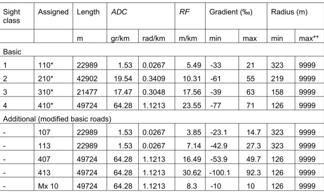
In EVA there are separate energy speed related functions per road alignment class. In total there are four road alignment classes. The classes are called sight distance classes. Sight distance class 1 has the longest sight distance. The sight distance will increase when the gradient decrease or the horizontal radius increase. The sight distance classification shall not be regarded as literally. For example a sinuous road in an open landscape will have a long sight distance but will have another sight class than 1. In order to describe the four sight classes six road alignment descriptions are used, see table 2.2.

(18)

Table 2.2 Road alignment standard for EVA roads.

Type road Length (m) Sight class ADC (°/km) RF (m/km)

LF_typ11 22 989 1 1.53 5.49

LF_typ12 22 009 2 (straight, rolling) 9.80 15.36

LF_typ21 20 893 2 (sinuous, plane) 29.8 5.00

LF_typ22 21 477 3 (sinuous;rolling) 17.47 17.56

LF_typ3x 25 149 4 (sinuous;rolling) 85.63 18.28

LF_typx3 24 575 4 (sinuous, hilly) 42.43 28.98

The four sight classes are based on in total six road descriptions:  scl 1: LF_typ11

 scl 2: 50% LF_typ12 and 50% LF_typ21  scl 3: LF_typ22

 scl 4: 50% LF_typ3x and 50% LF_typx3.

In order to classify road links into sight classes one can use definitions in table 2.3.

Tabel 2.3 Road alignment for sight class 1–4.* Sight

class Proportion of road with sight>500m

Alignment Longest gradient Max

gradient (%) Horizontal (rad/km) Vertical (m/km) Length (m) Average gradient (%) 1 >60% 0–0.5 0–10 2 160 0.8 2.1 2 35–60% 0.3–1.0 5–30 2 200 2.0 3.3 3 15–35% 0.7–1.3 >20 2 290 3.2 3.4 4 0–15% >1.3 >20 2 680 3.4 5.1 *(Carlsson, 2007)

There is need for more simple and clear definitions in order to classify into sight class, see table 5.5.

(19)

2.2.3 Fc functions for a dry road surface

In figure 2.1–2.3 the Fc functions of the EVA model is illustrated per sight class.

0.04 0.045 0.05 0.055 0.06 0.065 0.07 0.075 0.08 0.085 0.09 60 70 80 90 100 110 120 km/h L/ k m 1 2 3 4

Figure 2.1 Fc for car (C), EVA, per sight class (scl 1 – scl 4).

0 0.05 0.1 0.15 0.2 0.25 0.3 0.35 50 60 70 80 90 100 110 L/ k m 1 2 3 4

(20)

0.3 0.35 0.4 0.45 0.5 0.55 0.6 0.65 0.7 60 70 80 90 100 km/h L/ k m 1 2 3 4

Figure 2.3 Fc for truck with trailer (B), EVA, per sight class (scl 1 – scl 4).

These “functions” are expressed as table values in EVA. When calculating these values with the VETO model a series of desired speed values have been selected covering a speed interval big enough for the planning need. The resulting speed cycle per input desired speed only represents interactions between the vehicle and the road alignment. Still these “functions” are used in EVA to describe also interactions between vehicles. One can notice that increasing vehicle weight increases the relative difference in Fc between sight class functions.

2.2.4 Speed model

In EVA there is a parallel speed model to the Fc model. Speed is calculated as a function of:

 road width  speed limit  sight class  traffic flow.

This speed model is documented in (Carlsson, 2007). The output speed from this model is used as input to the Fc model.

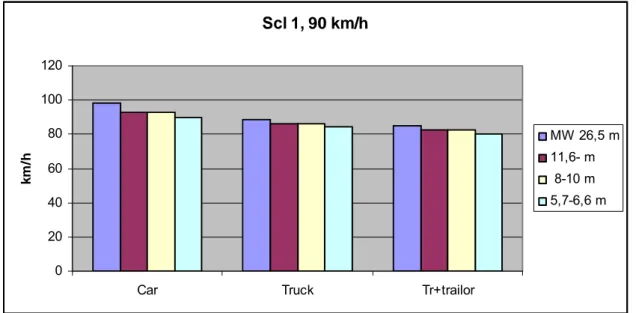
Examples describing the influence from road width and alignment standard are presented in figure 2.4 and 2.5.

(21)

Scl 1, 90 km/h 0 20 40 60 80 100 120

Car Truck Tr+trailor

km /h MW 26,5 m 11,6- m 8-10 m 5,7-6,6 m

Figure 2.4 Free flow speed and road width at alignment standard scl 1 and speed limit 90 km/h (EVA model). Width 8-10m 0 10 20 30 40 50 60 70 80 90 100

Car Truck Tr+trailor

km /h scl1 scl2 scl3 scl4

Figure 2.5 Free flow speed and road alignment standard (scl x) at road width 8–10 m (EVA model).

The influence of sight class on speed is bigger between scl 3 and scl 4 compared to the differences between scl 1, 2 and 3. For a car and a heavy truck the speed reduction from

(22)

2.3 Exhaust emissions as a function of road conditions, driving

behaviour and vehicles

In (Hammarström and Karlsson, 1988) analyses were made in relation to a situation “at present”:

 average vehicle descriptions per vehicle category  the Swedish rural road network

 average driving behaviour etc.

In the calculations there are typical driving behaviour related to the road design. The importance of Swedish road standard for traffic energy use is expressed of table 2.4–2.6. The saving potential is expressed in relation to most hypothetic situations with no gradients or no horizontal curves.

Table 2.4 Traffic energy use and speed index on rural roads for different conditions for cars.

Situation Fuel Speed

“at present” 1.00 1.00

No gradients .988 1.000

No curves 1.000 1.009

Table 2.5 Traffic energy use and speed index on rural roads for different conditions for truck+tr.

(23)

Table 2.6 Traffic energy use and speed index on rural roads for different conditions for bus interurban.

No curves .975 1.012

Table 2.4–2.6 express that road alignment is more important for heavy vehicles compared to light vehicles. The alignment improvements have increased speed and decreased Fc. The increased speed has given an increasing contribution to Fc but the resulting effect still is reduced Fc. Especially for truck with trailer there is a

considerable speed increase which probably has reduced the Fc reduction.

An analysis of other than dry road conditions is also included i.e. the effect of water, ice and snow on the road. The driving behaviour from ice and snow is included i.e. a speed reduction. The resulting effect per year for the total rural network is estimated to less than 1% increase compared to a dry road surface all year long.

2.4 IERD

The IERD project (EU) included both energy use for construction and for the traffic. The energy use for the traffic, the method used, is documented in (Hammarström, 2005). For calculations of traffic energy VETO was used. For road design, alignment input data to VETO, the MX ROAD program was used. MX ROAD also supplied most of the data for estimation of road construction energy.

Each country participating in the IERD project has supplied road data for at least two road objects, se table 2.7. In table 2.7 integrated measures for alignment are included.

(24)

Table 2.7 Road objects evaluated in the IERD project.

Road & Route

Option Total Route Length (km)

Typical cross section Speed Limit (km/h) ADC* (degrees/km) RF** (m/km) Czech Republic Czech Republic 1 16.73 MW 130 12.1 23.4 Czech Republic 2 16.0 MW 130 12.6 25.0 France France East 13.45 7 m 90 40.5 11.9 France Grand East 16.60 7 m 90 30.2 7.5 France West 12.53 7 m 90 21.0 7.7 France Grand West 12.79 7 m 90 17.6 11.2 Ireland Ireland 01 12.57 15 m 100 19.8 14.0 Ireland 02 12.37 15 m 100 17.9 14.1 Ireland 03 11.43 15 m 100 24.0 17.3 Ireland 04 11.45 15 m 100 25.6 16.6 Ireland 05 13.13 15 m 100 29.5 14.1 Portugal Portugal 1 15.60 MW 100 48.0 38.3 Portugal2 15.90 MW 100 42.7 33.2 Sweden Sweden bridge 5.70 MW(18.5) 90 32.4 11.7 Sweden tunnel*** 5.70 MW(18.5) 90 32.0 11.9

*ADC: Average Degree of Curvature;**RF: Rise and Fall.;***Road alignment available for the tunnel section from NRA. The other sections estimated by VTI.

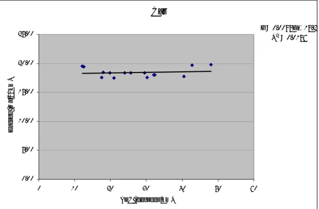
The importance of ADC and RF for energy use have been analyzed, see figure 2.6–2.9. The correlation between ADC and RF for the project routes is 0.37 i.e. to some extent the variation of energy use with one variable at the same time also describes the variation with the other variable.

(25)

Car y = 0.0098x + 18.2 R2_{= 0.0186} 0.00 5.00 10.00 15.00 20.00 25.00 0 10 20 30 40 50 60 ADC (degrees/km) E n erg y ( M J/ 10 km)

Figure 2.6 Energy use as a function of horizontal alignment, ADC, for EU cars. Car y = 0,082x + 17,056 R2_{= 0,8923} 0,00 5,00 10,00 15,00 20,00 25,00 0 10 20 30 40 50 RF(m/km) E n erg y (M J/ 1 0km)

(26)

Truck+trailer y = 0,492x + 97,821 R2_{= 0,1928} 0,00 20,00 40,00 60,00 80,00 100,00 120,00 140,00 160,00 0 10 20 30 40 50 60 ADC(m /km ) E n er g y (M J/ km )

Figure 2.8 Energy use as a function of horizontal alignment, ADC, for EU truck with trailer. Truck+trailer y = 1,2828x + 89,077 R2_{= 0,909} 0,00 20,00 40,00 60,00 80,00 100,00 120,00 140,00 160,00 0 5 10 15 20 25 30 35 40 45 RF(m/km) E n erg y (M J/ km)

Figure 2.9 Energy use as a function of vertical alignment, RF, for EU truck with trailer.

The conclusion of figure 2.6–2.9 is that ADC is of minor and RF of major importance for energy use. The influence of RF in this analysis might have been underestimated since the effect of special driving behavior in downhill gradients not has been noticed. This is of importance if there is an influence on the speed entering the road section following after the downhill section.

(27)

If ADC increases by 10% from the IERD average, 26 degrees/km, energy use will increase:

 by 0.14% for cars

 by 1.2% for truck with trailer.

If RF increases by 10% from the IERD average, 14 m/km, energy use will increase:  by 0.63% for cars

 by 1.7% for truck with trailer.

By changing the road alignment the specific energy use is influenced. An extreme such analysis is to:

 eliminate all gradients or  eliminate all curves or

 eliminate all gradients and all curves.

Such an analysis is presented in table 2.8. For this analysis the “worst” alignment per country has been used.

(28)

Table 2.8 Energy and speed index (100: original alignment) for changes in road alignment.*

Road object Energy Speed

Orig. No gradients No curves No gradients

and curves Orig. No gradients No curves No gradients and curves Car Czech v2 100 99.5 100.0 99.5 100 102.4 100.0 102.4 France East 100 98.3 99.4 97.8 100 100.0 102.4 102.4 Ireland 3 100 98.9 100.0 98.9 100 100.8 100.9 101.6 Portugal sol1 100 97.0 100.5 97.5 100 106.9 101.6 109.3 Sweden bridge 100 99.4 100.0 99.4 100 100.1 100.4 100.5 Truck Czech v2 100 81.9 100.0 82.0 100 102.4 100.0 102.4 France East 100 96.1 95.8 92.1 100 100.6 102.0 102.7 Ireland 3 100 83.4 99.3 83.1 100 102.2 100.5 102.7 Portugal sol1 100 78.6 99.8 80.0 100 109.2 100.7 110.7 Sweden bridge 100 98.6 99.9 98.2 100 100.6 100.3 100.9 Truck+trailer Czech v2 100 82.2 100.0 82.3 100 104.0 100.0 104.0 France East 100 93.9 96.3 90.5 100 101.1 102.0 103.1 Ireland 3 100 87.7 99.7 87.5 100 102.3 100.5 102.8 Portugal sol1 100 68.8 99.9 69.5 100 110.6 100.7 111.9 Sweden bridge 100 95.7 99.9 95.3 100 100.4 100.2 100.7

*Worst alignment, expressed as ADC and RF, per country; EU vehicles.

As could be expected the biggest potential for reductions is valid for Portugal sol1, the road with the highest values both for ADC and for RF, see table 2.8. An effect not included in table 2.8 is the change in link length when alignment, especially the horizontal curvature, is changed.

(29)

Table 2.9 Energy and speed index (100: original alignment) for changes in max gradient. Swedish road, bridge.*

Gradient (‰)

Energy(/distance) Speed**

Car Truck Truck+tr Car Truck Truck+tr

Base 100 100 100 100 100 100

Max 30 99.4 99.2 98.8 100.1 100.1 100.1

Max 20 99.4 97.6 97.7 100.1 100.6 100.4

*EU vehicles.;**As a function of vehicle performance.

Table 2.10 and 2.11 illustrates that the importance of gradient increases with the weight of the vehicle.

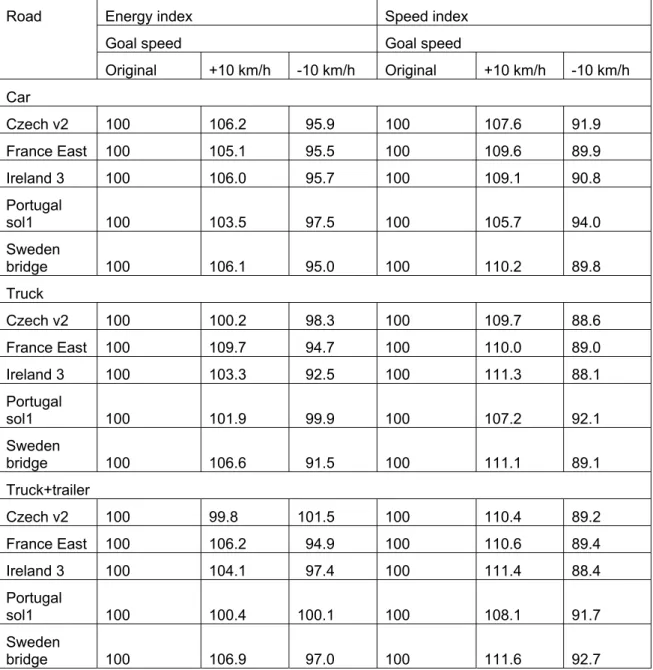
In table 2.10 the influence of speed isolated is presented. Desired speed has for all vehicle types been increased and decreased respectively by 10 km/h. These changes in speed can represent different measures influencing speed.

(30)

Table 2.10 Energy and speed index (100: original speed) for changes in desired speed.*

Road Energy index Speed index

Goal speed Goal speed

Original +10 km/h -10 km/h Original +10 km/h -10 km/h Car Czech v2 100 106.2 95.9 100 107.6 91.9 France East 100 105.1 95.5 100 109.6 89.9 Ireland 3 100 106.0 95.7 100 109.1 90.8 Portugal sol1 100 103.5 97.5 100 105.7 94.0 Sweden bridge 100 106.1 95.0 100 110.2 89.8 Truck Czech v2 100 100.2 98.3 100 109.7 88.6 France East 100 109.7 94.7 100 110.0 89.0 Ireland 3 100 103.3 92.5 100 111.3 88.1 Portugal sol1 100 101.9 99.9 100 107.2 92.1 Sweden bridge 100 106.6 91.5 100 111.1 89.1 Truck+trailer Czech v2 100 99.8 101.5 100 110.4 89.2 France East 100 106.2 94.9 100 110.6 89.4 Ireland 3 100 104.1 97.4 100 111.4 88.4 Portugal sol1 100 100.4 100.1 100 108.1 91.7 Sweden bridge 100 106.9 97.0 100 111.6 92.7

*Worst alignment, expressed as ADC and RF, per country. EU vehicles.

In table 2.11 the influence of desired speed is expressed by speed limit variation. The speed levels at different speed limit levels are based on speed measurements.

(31)

Table 2.11 Energy and speed index (100: original speed limit) for changes in speed limit. Swedish road, bridge.

Speed limit Energy Speed

Car Truck Truck+tr Car Truck Truck+tr

90 km/h* 100 100 100 100 100 100

70 km/h 93.3 94.2 99.5 85.4 93.7 97,3

*Max allowed speed for speed limit 90 km/h: car, 90 km/h; truck, 90 km/h; truck+trailer, 80 km/h.

Swedish road vehicles per category are different from average EU vehicles.

If the same constant speed is used uphill and downhill it is possible to estimate limit values for the gradient, see table 2.12. Outside these limits the gradient will cause extra energy use.

Table 2.12 Gradient limits (‰) for no extra energy caused by gradients at the same constant speed uphill and downhill.*

Desired Gradient limits (‰)

speed Car HGV Proportion HGV (%)

km/h 5 10 15

70 24 10 23 23 22

90 32 12* 31 30 29

110 42 12* 40 39 37

*Swedish car and swedish truck+trailer.

2.5 ECRPD

In the ECRPD project (EU) energy for road surface management were added to the IERD results. Like in IERD there were separate energy models for road measures and for the traffic. Of special interest for MIRIAM is the result from the rolling resistance measurements. Rolling resistance was estimated based on coastdown measurements (Hammarström et al, 2008), see table 2.13.

Table 2.13 Parameter values for a car in the general model.*

Cr01** Cr02** C2 C3 C4 C5

0.00926 0.0000695 0.000380 3.47E-05 0.00221 0.000111

(32)

dependent. Instead there is a separate term for temperature adjustments included in the

Cr function.

The main objective in most measurements of rolling resistance and road surface influence is to reach a general model representative for one category of vehicles. In ECRPD the parameters C2–C5 represents the test vehicle and Cr01 and Cr02 are most rough estimations for an average car.

The ECRPD project, the Swedish part, included 28 test routes for coastdown

measurements. These were selected to cover most of the existing variation in iri and

mpd. The range of variation is a function of the road length the measure represents. In

the ECRPD case the finest resolution is 20 m, see table 2.14.

Table 2.14 Data range in ECRPD at coastdown measurements*

iri (m/km) mpd (mm) At 20 m average At 400 m average At 20 m average At 400 m average Min .59 .79 .26 .39 Max 8.75 3.66 2.74 2.54 *28 test routes.

2.6 Production

measurements

On commitment of the Road Administration VTI has performed further rolling

resistance measurements beyond the ECRPD in the “Production measurement project”, see (Karlsson et al., 2011). These measurements include coastdown measurements both with a car and with a heavy truck. What is special with this study compared to ECRPD:

 more efforts on HGV

 both summer and stubbed tyres for the car

 varying the vehicle mass in order to isolate transmission losses from rolling resistance in the analysis

The documentation of this project includes both results from the study measurements and some other data sources.

In section 3 there is more information about this study.

2.7 Coastdown with 60t truck with trailer

In order to estimate exhaust emission factors to ARTEMIS/HBEFA there is need for driving resistance parameters including rolling resistance.

Coastdown measurements were performed with a 60t truck with trailer and a box vehicle body, see (Hammarström et al, 2011). In order to isolate transmission losses from Cr two vehicle loads were used. The estimated rolling resistance parameters:

(33)

Cr=(0.00375+0.0000916*iri*v+0.000659*mpd) (the mpd parameter is not significant different from zero (95%))1

These estimated parameters are based on measurements on just one test route in both directions (800 m). The test route includes RST data per 20 m section in both driving directions. What makes these results of interest, in spite just one test route, is the trailer. The trailer characteristics:

 air suspension system  super single tyres.

Empirical data from just one test route make the estimated road surface effects most unsecure. The study also included estimation of air and transmission resistance. Especially the air resistance estimate including side wind effects has a low degree of uncertainty.

2.8 Average speed and the influence of road surface

The driving pattern is influenced of the road surface in two ways: physical and by driving behaviour. The influence from road surface conditions on average speed is described in (Ihs and Velin, 2002).

Car, daytime:

Vpb=79.47 – 0.11*rut – 1.33 * iri – 4.98 * NARROW – 0.71 * NORMAL + 14.07 * HG90 + 28.46 * HG110 + 3.16 * MV

Heavy truck, daytime:

Vlb = 77.1 – 0.12 * rut – 1.17 * iri – 3.48 * NARROW – 0.62 * NORMAL + 9.97 * HG90 + 16.33 * HG110 + 1.77 *MV

Truck with trailer, daytime:

Vlbs= 74.5 – 0.09 * rut – 2.31 * iri – 0.71 * NARROW + 0.37 * NORMAL + 10.55 * HG90 + 13.43 * HG110 – 0.45 * MV

Vpb: average speed for light vehicles (km/h) Vlb: average speed for heavy vehicles (km/h)

Vlbs: average speed for heavy vehicle with trailer (km/h) rut: rut depth (mm)

(34)

HG90: 1 if speed limit=90, else 0 HG110: 1 if speed limit=110, else 0

Then there are two road surface measures influencing the speed: rut and iri. The iri effect is presented in figure 2.10.

Speed reduction and iri

0 2 4 6 8 10 12 14 16 0 1 2 3 4 5 6 7 iri km /h car heavy tr heavy tr+tr

Figure 2 10 Speed reduction as a function of iri (Ihs and Velin, 2002).

The study did not include the mpd measure.

2.9 INKEV

The possibilities to include ECRPD results into Swedish road planning have been investigated in the INKEV project (Ramböll, 2011). The INKEV report includes:

 a critical analysis of different ECRPD sub models  a test of the ECRPD tool for one Swedish road object.

The results for the Swedish road object were not in contradiction to the main results from ECRPD.

This report highlights the considerable difference in energy use between maintenance and traffic energy. The quote between traffic and maintenance energy for motorways is estimated to approximately 1000 for Swedish road vehicles.

2.10 Conclusions based on literature

Conclusions from the literature:

 For Swedish road conditions one cannot expect big relative traffic energy changes from road alignment or road surface changes

 There is a road surface effect both on RR and v

 The energy importance of road alignment increases with vehicle weight

 It is possible to formulate guidelines for the selection of an energy efficient max gradient based on the speed limit and distribution of traffic on type of vehicles  It is important to notice for road gradients that the important condition for a

(35)

RF value. In most cases there will be a high correlation between these two gradient measures

 Ice and snow on rural roads has been estimated to increase total Fc by approximately 1%

 The traffic energy saving potential needs to be regarded in parallel to the road change energy

 Especially road maintenance changes on high traffic roads contributing to lower

Fc should as a general rule always be energy efficient in total

 Since most road measures influence Fc by more than one way, for example both by RR and by speed, it is not that obvious what will happen to Fc since the effects in general are small

 There is a considerable amount of RR measuring data available in the same form creating a possibility for a total analysis of Cr parameter values.

(36)

3 A general rolling resistance model per vehicle category

3.1 Introduction

Based on data from other projects a general rolling resistance model has been developed for the MIRIAM sp2 analysis. Essentially, the same model has been used for all vehicle categories. Separate parameter values for a car, a heavy truck and HGV trailer have been estimated.

The final RR model for MIRIAM is based on measurements done in previous projects:  coastdown data from three projects: ECRPD; 60t and Production measurements.  drum measurements.

In the following subsections we summarize the RR model for three vehicle categories and describe in some detail how the parameter values have been estimated.

3.2 Estimation of a general RR model for a car

The final RR model for a private car, used in this report, heavily rests on the work by (Karlsson et al, 2011). We here summarize the method that was used by them and what modifications of their results that have been done in Miriam.

Basically, the coastdown method was applied to estimate the RR parameters for two different tyres. From earlier projects (ECRPD and Production measurements) a large number of coastdown measurement data was available. Essentially, the following model was used:

y = Fz * ( Cr00 + CrTemp*(5-T) + CrMPD*mpd + CrIRI*iri + CrIRIV*iri*(v-20) ) +

CrSide*Fy^2 + CL*AIR + CLbeta*AIR*sin(beta) (3.1)

where

Crxx and CLxx are model parameters to be estimated by regression y is the decelerating force acting on the vehicle (adjusted for gravitational

forces and transmission losses)

T is the air temperature

mpd is mean profile depth (road macrotexture)

iri is the International Roughness Index (road unevenness) v is velocity [m/s]

Fy is the side force acting on the vehicle AIR = Ayz * VLR^2 * dns / 2 * cos(beta) Ayz is the cross section area of the vehicle

VLR is the resultant air speed (relative to the vehicle) dns is the air density

beta is the angle between the vehicle velocity and the resultant air

(37)

Note that RR only comprises the terms containing Cr00, CrTemp, CrMPD, CrIRI and

CrIRIV.

A disadvantage with model (3.1) is that it is unphysical in the sense that the RR

contribution from unevenness (iri) does not tend to zero when iri tend to zero. In order to avoid this defect, the two iri terms can be replaced by a single term

CrIRI_V_EXP*iri*V.

y = Fz * ( Cr00 + CrTemp*(5-T) + CrMPD*mpd + CrIRI_V_EXP*iri*v) ) +

CrSide*Fy^2 + CL*AIR + CLbeta*AIR*sin(beta) (3.2)

Another difficulty is that both models (3.1) and (3.2) require that the decelerating force,

y, is adjusted for transmission losses. The transmission losses are modelled as a constant

force, C0, independent of the weight of the vehicle2. In the work by (Karlsson et al, 2011), transmission losses were estimated using special coastdown measurements with varying vehicle weights. to 65.5 N. The resulting value, C0=65.5 N, was, however, very unreliable. In hindsight, this value is probably too large and a more reasonable value is probably 40 N.

A further circumstance that should be noted is that the above models were estimated for two types of tyres only, normal Michelin Energy and stubbed winter tyres. Most of the measurements were done using the Michelin Energy tyres. For the Miriam project it was desirable to modify the parameters to better correspond to a representative vehicle. From drum measurement data covering 90 different tyres, it was found that the mpd coefficient, CrMPD, for the Michelin Energy tyre was fairly representative (slightly lower than the average value). On the other hand, the basic rolling resistance was untypically low. Therefore an adjustment of the coefficient Cr00 was done. Drum measurement data indicated3 that Cr00 for a representative vehicle can be expected to exceed the probe tyres by 1.67e-3.

In Table 3.1 estimated parameters for models (3.1) (columns A, B and C) and model (3.2) (columns D and E) are shown. In column A, the original parameter estimations made in (Karlsson et al, 2011) are displayed. In column B, corresponding estimations using a more reasonable value for the transmission losses (C0=40 N instead of 65.5 N). It is evident that only the basic rolling resistance (Cr00) is affected, while all other terms are virtually unchanged. This is due to the large correlation between the

transmission resistance and the basic rolling resistance (the vehicle weight varies only by a small amount between the measurements). In column C, Cr00 has been adjusted to a more representative value, as indicated by drum measurement data. In columns D and E, values corresponding to columns B and C are shown, but for model (3.2) instead of model (3.1).

(38)

Table 3.1 Parameters for model (3.1) obtained by (Karlsson et al, 2011) and for model (3.2) computed in Miriam Sp2. Reference temperature is 5°C. (Additional dummy terms included in the regressions are not shown here.)

A B C D E

C0 65.5 N 40 N 40 N 40 N 40 N

Cr00 6.48E‐03 8.02E‐03 9.69E‐03 Cr00 7.76E‐03 9.43E‐03 CrTemp 1.04E‐04 1.03E‐04 1.03E‐04 CrTemp 1.04E‐04 1.04E‐04 CrMPD 1.72E‐03 1.72E‐03 1.72E‐03 CrMPD 1.72E‐03 1.72E‐03 CrIRI 4.66E‐04 4.66E‐04 4.66E‐04 CrIRI_V_EXP 2.10E‐05 2.10E‐05 CrIRI_V 3.65E‐05 3.65E‐05 3.65E‐05

CrSide 2.52E‐05 2.51E‐05 2.51E‐05 CrSide 2.45E‐05 2.45E‐05 CL 0.4257 4.26E‐01 4.26E‐01 CL 4.36E‐01 4.36E‐01 CLbeta 0.5446 5.43E‐01 5.43E‐01 CLbeta 5.44E‐01 5.44E‐01

The alternative D has been used for the general tyre model, see section 6.1.

3.3 Estimation of a general RR model for an HGV

In (Karlsson et al., 2011) coastdown measurements were done also for an HGV without a trailer. Unfortunately, due to measurement errors the resulting parameter estimations were rather unstable. For this reason no final model was formulated.

In (Hammarström et al., 2011) measurements were done for both a truck and a trailer. Although some interesting results concerning the air resistance were obtained, the results describing the influence of road surface conditions on RR were very unreliable. In order to obtain some results a renewed analysis based on a merged dataset from the two reports was performed. A crucial difficulty is that the modelling details can be varied in a large number of ways and that the results vary a lot when changing the implementation details. These instabilities make it difficult to confidently determine a final model.

The model results for the HGV is unstable in a number of ways. Firstly, an upper limit for acceptable wind speed, Wmax, can be set to different values. The model parameter estimations varied with this choice. Secondly, the temperature coefficient, CrTemp, is unknown4 for the HGV. The model parameter estimations also vary with this choice. Thirdly, even more alarming, the model was unstable with respect to removing data from a single road strip.

By carefully analyzing the ranges in which the model parameters varied when the above conditions were changed within reasonable limits, a “best” set of parameter values displayed in Table 3.4 was finally selected for the Miriam model.

(39)

Table 3.2 Parameters for a modified version of model (3.2). Reference temperature is 8°C. (Additional dummy terms included in the regressions are not shown here.) The suffix “_t”means truck only, while “_tt” denotes truck + trailer.

C0* 260 N Cr00_t 4.14E‐03 Cr00_tt 3.65E‐03 CrTemp* 3.00E‐05 CrMPD 1.02E‐03 CrIRI_V_EXP 1.58E‐05 CL_t* 0.5358 CLbeta_t* 0.3661 CL_tt* 0.895 CLbeta_tt* 1.411 *Not estimated by regression.

For the vehicle simulation program the coefficient Cr00_tt for the combination

truck+trailer is inconvenient. More appropriate is to separate the basic rolling resistance coefficient for the trailer from that of the truck. This can be achieved by equating the (basic) rolling resistance force acting on the entire vehicle with the corresponding sum of forces for the truck and for the trailer. Using the value for Cr00_t and the mass for the truck (15.1 ton) and for the trailer (12.3 ton), yields:

Cr00_trailer = 0.00306

It should once again be noted that the estimated values are very uncertain. Also, no consideration to the representativity of the tyres was taken.

(40)

4 A fuel consumption model

4.1 Fuel consumption models in general

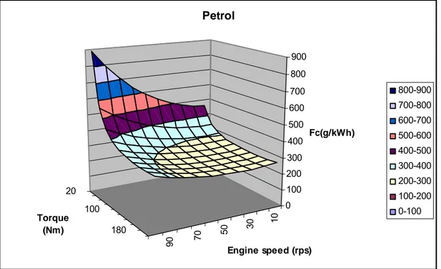
Fuel consumption is a function of driving resistance and engine efficiency. The engine efficiency is a function of engine speed and engine torque:

 Increasing engine speed will reduce engine efficiency  Increasing torque will increase engine efficiency.

At idling, for example, the efficiency is equal to zero. The engine efficiency, expressed as gram fuel per kWh, is a non linear function of engine speed and out torque, see figure 4.1. 10 30 50 70 90 20 100 180 0 100 200 300 400 500 600 700 800 900 Fc(g/kWh) Engine speed (rps) Torque (Nm) Petrol 800-900 700-800 600-700 500-600 400-500 300-400 200-300 100-200 0-100

Figure 4.1 Engine map (g/kWh) for petrol engine. Engine specification: petrol; year model 1996–2003; max engine power100 kW; displacement=1.95 dm3.

Driving resistance is a function of the road conditions and driving behavior. Engine speed is a function of vehicle speed and gear position including gear ratios. Engine out torque is a function of the driving resistance, the transmission and throttle opening. The transmission influences the out torque in two ways: transmission losses and the gear position. If a lower gear is selected the engine speed will increase and the torque will decrease.

In order to estimate fuel consumption for an engine the engine internal friction also is of importance.

The function demonstrated in figure 4.1 can also be expressed as the consumption of fuel per time unit (Fct). The function needed to express Fct as a function of engine speed and torque is a product of two polynoms.

(41)

In (Hammarström and Yahya, 2011) an Fc model with a high degree of explanation is presented:

Fct=c0*(Mind+c1*Mind2+c2*Mind3)*(NRs+c3*NRs2+c4*NRs3) Mind=(PME+ PFR)/ (NRs*6,28)

PME: engine power

PFR: engine internal friction PME=PAUX+ PTRM+PDRIV PTRM: transmission losses (W) PDRIV= Fx * v

Fx: driving resistance (N)

The resulting Fc function will be complicated if all important variables will be included in parallel. One problem is how to describe transmission losses. These losses will change between gear positions. A change of gear position will result in a discrete change in Fc. Gear position could be one variable in a function but the use of such a function will be complicated. Another alternative could be to express gear position as a function of vehicle speed.

4.2 Driving

resistance

The driving resistance (Fx) constitutes a sum of forces:

Fx = Fb + Fair + Facc + Fgr + Fside + Fr Fx: total driving resistance5

Fb: wheel bearing resistance (N) Fair: air resistance (N)

Facc: acceleration resistance from vehicle mass (N) Fgr: gradient resistance (N)

Fside: resistance caused by the side force (N) Fr: rolling resistance (N)

Wheel bearing resistance:

In the wheel bearings there will be a resistance proportional to the vertical force (Mitschke, 1982):

(42)

Fz: vertical load per tyre (N) Air resistance:

The air resistance at calm wind conditions is expressed by:

Fair = Cd*Ayz*dns*v2/2

Where

dns= (348.7/1000)*(Pair/(T+273)) v: the vehicle velocity (m/s)

dns: the density of air (kg/m3)

Ayz: the projected frontal area of the vehicle (m2)

Cd: the air dynamic coefficient (dimensionless) Pair: the air pressure (mbar)

T: the ambient temperature (°C) Inertial force:

Facc=macc*dv/dt macc=m+mJ

dv/dt: the acceleration level (m/s2)

m: the total mass of the vehicle (kg)

mJ=sum(KJ*J/rwh2), where sum means summation over the wheels (kg)

rwh: the wheel radius (m)

J: the inertial moment per wheel (kgm2)

KJ ( set to 1.0 in this study): a correction factor of J to include moving parts in the transmission system.

Gradient resistance:

Fgr=m*9.81*sin(gr)

where

(43)

Side force resistance:

Fside=Fy*Cr3

where

Fy=m*(cos(crf/100)*v2/R-9.81*sin(crf/100)*cos(gr)) Cr3=1/CA

Fy: the side force acting on the vehicle (N) CA: the tyre stiffness parameter (N/rad)

crf: the crossfall (%)

gr: the longitudinal slope (rad)

R: the radius of the road curvature (m)

Cr3: the estimated parameter for the stiffness inverse (rad/N)

The cross fall causes a driving resistance (Fside) because the tyre will not be parallel to the vehicle movement direction. Fside is a function of Fy and CA. CA is a non linear

function of the tyre load. Because of the cross fall one can expect different Fside on different wheels on the same wheel axle. This level of detail has not been used in the analysis.

The cross fall of the road will influence the normal force distribution from left to right. Higher vertical force on the right side is expected to give higher tyre temperature and pressure on the right hand side of the vehicle.

Rolling resistance:

The following basic model will be used in this report:

Fr= Cr*m*9.81

There are several alternatives to express Cr as a function of other variables. The following alternative will be used for the Fc model in this study:

(44)

where

iri: the road roughness measure (m/km) mpd: the macrotexture measure (mm) m: the vehicle mass (kg)

v: the vehicle velocity (m/s)

Cr0, Cr1 and Cr2: the rolling resistance parameters.

4.3 Proposal for fuel consumption models

4.3.1 An instantaneous model

By combining section 4.1 and 4.2 it would be possible to develop an Fc function able to describe most of the effects of interest in road planning. The main problems to solve are that direct information about engine speed and torque not are available. Instead these variables are expressed indirectly by vehicle speed and driving resistance.

An Fc function based on section 4.1 is:

Fct=c0*Minde1*NRse2 Fct: Fc per time unit

Mind=( PFR +PME)/ (NRs*6,28) PME=PAUX+ PTRM+PMdriv PMdriv= Fx * v PFR=k1*NRs PAUX=k2 PTRM= k3*NRs Mind=(k1*NRs+k2+ k3*NRs+ Fx * v/VGVX)/(NRs*6.28)

In a simplified Fc model engine speed and torque need to be expressed indirectly.

k4=(k1+k3)/6.28

Mind=k4+k2/(NRs*6.28)+k5*Fx=k4+k21/NRs+k5*Fx Fct=c0*(k4+k21/v+k5*Fx)e1*(k6*v)e2

This function can be expressed in an alternative way:

Fct=c1*(1+k21/v+k7*Fx)e1*ve2 Fcs=Fct*v

The function is only valid for Mind≥0. Mind<0 represents a situation when full engine brake is used in combination with the use of wheel brakes. Fct then should be

(45)

Depending on what demand for use of the function Fx can be expressed to meet that demand.

In order to describe Fx representative vehicle parameters are used as far as possible. The other parameters – c0, k4, k21, k5, k6, e1 and e2 – are possible to estimate if Fct for different driving conditions are available. Such values are possible to calculate by use of for example VETO.

To a great extent this function approach should be able to describe the same effects as programs like VETO. What cannot be described is that the vehicle situation in one road and time position is a function of the conditions in the position before. The transmission losses and the relation between vehicle speed and engine speed are described in a most simplified way with loss of accuracy.

The function approach is possible to use as a base for functions on different levels of complexity.

When developing an Fc function one can state that the big difference is between driving modes and integrated driving modes along a road. In the second alternative driving modes need to be described in some way for example by average speed.

In the function Fx needs to be expressed by measures possible to use in practice. At least iri and mpd needs to be included.

4.3.2 On a road link level

The same principals as in 4.3.1 can be used on a link level. Problems to solve:  influence of gradients

 influence of horizontal curvature  influence of other speed changes.

The problem is that on a link level gradients and curvature are available as simplified average values. There also is interdependence between these variables and road surface variables when estimating Fc.

On a link level the resulting gradient effect need to be described. To a big extent uphill and downhill will even out but not completely. The gradient effect corresponds to a change in transmission losses, a change in gear position, and brake energy. This brake energy is a function of:

 gradient

 rolling resistance  air resistance  vehicle mass.

Gradient brake energy will increase if:  the gradient increases

(46)

Increasing curvature will cause a change in energy use caused by:  the retardation level in front of the curve, brake energy losses  the side force resistance

 the speed difference between before and in the curve  the acceleration level after the curve

 the rolling resistance  the air resistance.

The resulting curve effect, retardation and acceleration, is most similar to the gradient effect i.e. expressed by brake energy losses before the curve. The main effect of the acceleration level is the influence on average speed.

The extra energy use for curvature will increase if:  the speed difference increases

 the retardation level increases  the air resistance decreases  the rolling resistance decreases.

The possibility to describe gradient and curvature effects depends on what measure is used to describe these road conditions. In this study rise and fall (RF) and average degree of curvature (ADC) will be used. These measures are not good enough for an exact expression of the energy process. There are also problems in order to describe Fc equal to zero, full engine brake, in one interval and different from zero in another interval.

For gradient and curvature there might be a decrease in energy use, because of the speed effect, compared to a horizontal and straight road if there is no use of the braking

system. The resulting effect is a function of all variables mentioned above and needs a model like VETO to be described in detail. The problem on a link level is then to express the average Fx. The approach needed:

Fx=Fair +Fr+g(ADC,Fair,Fr,v,dv/dt)+h(RF,Fair,Fr) ADC: average degree of curvature (rad/km)6

RF: rise and fall (m/km) g( ): the curvature term h( ): the gradient term

Such a function is complicated to express and most difficult to calibrate.

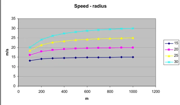
In the curvature term g speed is included in Fair and Fr but also in order to express the distance of retardation (s) and acceleration:

(47)

s=( vhc2 -v2)/(2*dv/dt)

vhc: the lowest speed in the curve is a function of v and the curve radius, see section

5.2.5

The final function approach calibrated on a link level:

Fct=c1*(1+k5*(Fr+Fair+d1*ADC*v2_+d2*RF+d3*RF2₎e1_*ve2

In this approach at least the speed interaction with curvature is included to some extent. The gradient interaction with speed – brake energy will decrease with increasing speed – is not included.

With this simplified approach one will lose the possibility to express that road surface effects to some extent are depending on ADC and RF but also that the influence of ADC and RF to some extent is depending on Fr and Fair.

4.3.3 For a driving cycle

A driving cycle constitutes a series of speeds for example on a second by second level. Such a series also includes full information about acceleration levels. Each traffic situations in HBEFA/ARTEMIS is represented by a driving cycle. There are different alternatives in order to develop Fc functions for driving cycles:

 by average speed

 by average speed and a measure to express speed changes and dv/dt  by a speed and acceleration matrix.

The first alternative is used in programs like COPERT, see (LAT, 2007). This program is similar to ARTEMIS/HBEFA but instead of traffic situations average speed is used for three classes of road types: urban, rural and motorway. For each such class there is a set of Fcs average speed functions. In MIRIAM at least mpd and iri variables are needed in addition to average speed.

The second alternative is similar to the first with the exception there is no need for different classes of functions. The main problem is how to develop a term describing speed changes and dv/dt. One such approach could be to use an estimation of brake energy.

With the matrix alternative there is need to calibrate this function: