The impact of immigration on the Swedish Economy

(1)

School of Business, Society & Engineering

Bachelor Thesis in Economics

The impact of immigration on the Swedish Economy

________________________________________________________

Samia Nasir & Elina Larsson

Supervisor: Clas Eriksson

(2)

Bachelor Thesis in Economics (NAA 303)

Date:

May 31st, 2018

Project Name:

The impact of immigration on the Swedish Economy

Authors:

Samia Nasir & Elina Larsson

Supervisor:

Clas Eriksson

Examiner:

Christos Papahristodoulou

Comprising:

15 ECTS credits

(3)

ABSTRACT

The flow of immigrants between Europe and many other countries is often brought up in the discussion of the labor market. It is also questioned whether an increased immigration is beneficial for the society and the economy of the receiving country.

This paper is an investigation of the above-mentioned problem “does immigration benefit a country’s economy and what are the effects of immigration on the economy?”. Furthermore, we will especially look at how immigration benefits the natives in the country with respect to labor and capital income. We will also investigate if there is a difference in education and skills between immigrants and natives and we will also examine the consequences of this. The discussion about benefits and liabilities to the society that has arisen, due to the welfare effects in the economy, will also be brought up and analyzed.

The thesis work will mostly be a study of theoretical findings, where we will discuss the previous researches and important models, for instance Borjas (1999), who uses a model that gives a solid result of how much natives benefit from immigration in term of labor and capital earnings. To support the theoretical part, we have gathered the data from Eurostat and Swedish migration Authority, which will help to find some empirical results as well. This paper also includes a regression model that measures the change in the unemployment rate where the independent variables are GDP growth rate and immigration inflow.

(4)

ACKNOWLEDGEMENT

We would like to express our special thanks to our supervisor Clas Eriksson for providing valuable comments and suggestions. The completion of this thesis could not have been possible without the guidance, patience and help of our supervisor.

Secondly, we would like to thank our families for the support and continuous encouragement.

(5)

1 INTRODUCTION

The area of study for our thesis is the impact of immigration on the developed economy (with a reasonably flexible labor market). According to Oxford dictionary, the word immigration

means the action of coming to live permanently in a foreign country. The study of immigration

and its effects is a significant area for both economics and politics. People immigrate due to several reasons like war, trade, work, education, safety etc. People also take decision to move from one country to another to improve their living standard (Swedish Migration Agency).

People who move because of war and political situations are the asylum seekers and some people move for job purpose. According to Statistics Sweden in 2017, 68898 people from over 160 countries became Swedish citizens out of which a large part (8635) of citizenship was granted to Syrian citizens. The immigration increased by 14 percent compared to 2016. Meanwhile, according to Swedish Public Employment Service 2017 has been a good year for the labour market. In 2017, 94000 people got jobs and the employment rates increased to 78.1 percent, which is highest in the EU. Meanwhile, the unemployment rate decreased to 6.7 percent1_.

With the increase in the immigration the population also increases. In 2004 the population of Sweden exceeded 9million for the first time. In 2017 Sweden crossed the 10million population mark as shown in Figure 1.

1_{The numerical information used in the introduction section is from Statistics Sweden website} https://www.scb.se/

(8)

2

Figure 1: Population 1800−2017 (SCB)

1.1 S

TATEMENT OF THE PROBLEM

In recent years, the flow of immigration has increased quickly due to several reasons. The reasons can be political, environmental or economic. The political and environmental reasons include refugees and asylum seekers who migrate due to war, natural disasters and poverty (Swedish Migration Agency). Economic reasons include when people move for the jobs purpose to improve their welfare.

One of the reason is non-stability in the home country, which has arisen a large discussion whether immigration is beneficial for receiving the country or not. Earlier findings and analyses have suggested that it is beneficial for the natives in the country, due to their different qualifications in contrast to the immigrants. However, other findings suggest that immigrants take jobs from natives. While previous research brings up whether immigrants “take jobs” from natives, it also stresses whether immigration lowers the wages or not. With the use of data regarding this, we ask the question, “how is this measured in Sweden”?

0 2,000,000 4,000,000 6,000,000 8,000,000 10,000,000 12,000,000 1800 1807 1814 1821 1828 1835 1842 1849 1856 1863 1870 1877 1884 1891 1898 1905 1912 1919 1926 1933 1940 1947 1954 1961 1968 1975 1982 1989 1996 2003 2010 2017 Po p u lat ion Years

(9)

3

1.2 O

VERVIEW OF HISTORY OF IMMIGRATION AND EMIGRATION IN

S

WEDEN

According to the Swedish Migration Agency, from the mid-1800s to the 1930s people emigrated from Sweden to US, Canada, South America and Australia, which leaves the deepest mark on the development of Sweden. Over 1.3 million Swedes moved because of poverty, religious persecution and lack of political freedom. The peak year of emigration was 1887 when more than 50,000 people left Sweden and most of them moved to America. After World War I, the emigration declined due to US restriction. After World War II, because of German, Nordic and Baltic refugees, Sweden changed from being a net emigration country into a net immigration country. Since 1930, Sweden has larger immigration than emigration2_.

Figure 2: Immigration and emigration 1960−2016 and forecast 2017−2060 (SCB)

As immigration increased after World War II, the Swedish Migration Agency was started in 1969 to deal with immigration matters. After World War II over 100,000 refugees from Yugoslavia moved to Sweden. In the 1980s the number of asylum seekers from the countries Iraq, Lebanon, Syria and Eritrea increased significantly in the Western Europe. In 1995 Sweden

2 _{The numerical values and information are from the Swedish Migration Agency website} https://www.migrationsverket.se/

The graph is from Statistics Sweden website.

0 20,000 40,000 60,000 80,000 100,000 120,000 140,000 160,000 180,000 200,000 1960 1970 1980 1990 2000 2010 2020 2030 2040 2050 2060 Forecast Immigration Emigration

(10)

4

joined the European Union and later in 1999 the European Council set a goal to make asylum and migration policy. In 2001 Sweden joined the Schengen Cooperation which today consists of 26 countries to grant visa free entry in the Schengen area (Swedish Migration Agency).

Figure 3: Residence permits granted 1980-2014 (Swedish Migration Agency)

1.3

A

IM

This paper is an investigation of how immigration effects a developed economy. The aim is to understand and analyse benefits and liabilities in the labor market for natives and foreign born. This is achieved by analysing two theoretical models that attempts to describe the change in wage level for natives when there is an inflow of immigration, originally built on Borjas (1999) and Altonji and Card (1991). Moreover, we examine how immigration affects unemployment, using Swedish data.

1.4 L

IMITATIONS

The thesis work is both theoretical and empirical. For the theory part, the study of economic articles and relevant theoretical methods will be used, whereas for the empirical part we will use data and statistics from reliable sources. The data are obtained from Statistics Sweden and

0 20000 40000 60000 80000 100000 120000 1980 -1989 1990 1991 1992 1993 1994 1995 1996 1997 1998 1999 2000 2001 2002 2003 2004 2005 2006 2007 2008 2009 2010 2011 2012 2013 2014

(11)

5

the Swedish Migration Agency. The empirical research and analysis of this paper will be restricted to Sweden.

1.5 L

ITERATURE

R

EVIEW

There have been many previous research studies done by other researchers around the subject of this paper and one of the leading author’s is George G. Borjas who has written a book about immigration economics as well as articles about the benefits from immigration. One of our multifactor models is built on Borjas (1999), who wrote an article that includes a model, trying to measure the change in wage level for natives when there is an inflow of immigrants to the labor market. The article measures the immigration surplus when there is a difference in skill level for the two groups, and when there is no difference. It distinguishes between the groups that is getting beneficial respectively the contradiction.

Altonji and Card (1991) wrote the article “The effects of immigration on the labor market outcomes of less-skilled natives”. The article includes a model that measures the wage level for natives when there is an inflow of immigrants but differs from Borjas model in the sense that it uses heterogeneous inputs instead of homogeneous. Their model is not totally different from other economist’s work, in the sense where they all basically are trying to measure the same thing; changes for the natives related to an immigration inflow. However, the model by Altonji and Card differ in two different key aspects, for instance, the inputs of their model consider both unskilled and skilled workers, and it also uses a locally produced good (call it 𝑌) to be measured. This is a heterogeneous model, where the author’s build some of the equations and derivations on earlier work by other economists, such as Johnsen (1980a). Although the model to some extent builds on earlier economist’s work, Altonji and Card (1991) clearly emphasize how their work differ from earlier studies.

(12)

6

Jennifer Hunt, Professor of economics has done a lot of previous research regarding immigration and the benefits of it, where she, for instance, stresses the controversial thought that immigration benefits the whole society, especially if immigrants are low skilled or possess different skills than the natives does (DN Fokus 2016).

Marjolaine Gauthier-Loiselle and Jennifer Hunt (2008) in the paper “How much does immigration boost innovation” have done research about immigrants, where they discuss to which extent skilled, highly educated immigrants increase innovation. This paper is especially dedicated to US but can to an extent be applied to Sweden as well. The empirical part of this study will consist of running five sample regression equations to see how the change in unemployment corresponds to changes in the GDP growth rate, and immigration inflow (refugees and labor force). This study is dedicated to Sweden only, because of the limited time. Although, we realize that other factors than those named above, also have an impact on the change in unemployment. For the five regression equations, two data sets will be encountered in the study; the first one is from the year 1990-2017 and considers immigration as one group. The other data set includes immigration as both refugees and work permits but is only measured from the year 2000-2017. The reason for the measure of two data set is as previously stated, that the second data set includes immigrants as two different groups, so it is interesting to see if this dataset has a different impact on the dependent variable that set one. Furthermore, the regression equations will start with Okun’s law. Where we look at the change in the dependent variable as a change in unemployment, caused by the independent variable as growth in GDP. Okun’s law (studied by Arthur M. Okun) shows a negative relationship between the unemployment and GDP.

(13)

7

2 THEORETICAL BACKGROUND

In the theoretical part, we have analyzed the problem statement by using models and explaining figures. It will give a picture of the effects of immigration for the natives on the labor market given that the immigrants are either low skilled or highly educated.

According to Borjas (2014) “immigration has consequences, and these consequences generally imply that some people will lose while others benefit” 3_.

This theoretical part is a brief introductory description of why people gain and lose in the case of immigration. It explains how immigrants affect the natives when they act as perfect substitutes or complements. This part also includes Cobb-Douglas production function, which explains that the increase in the labor due to immigration increases the rate of return to capital and decrease the real wage of natives. The natives always benefit from immigration either in the form of higher wages or in the form of an increase in the return of capital in the long run.

2.1 L

ABOR

M

ARKET

E

QUILIBRIUM

In the labor market, firms want to keep salaries low whereas workers prefer jobs with high salaries. Labor market equilibrium helps to create a balanced situation between workers and firms.

In the labor market, firms constitute the demand side of equilibrium whereas the workers determine the supply side. Equilibrium is the point where the supply of workers is equal to the demand of workers, which means anyone who wants to work can find a job.

(14)

8 Figure 4: Equilibrium in a Competitive labor market (Borjas,2016)

In the above figure 𝑤∗_{is the equilibrium wage, 𝐸}∗_{is the equilibrium employment and P is the} firm/producer surplus whereas Q is the worker surplus4.

2.2 L

ABOR

M

ARKET

I

MPACT

O

F

I

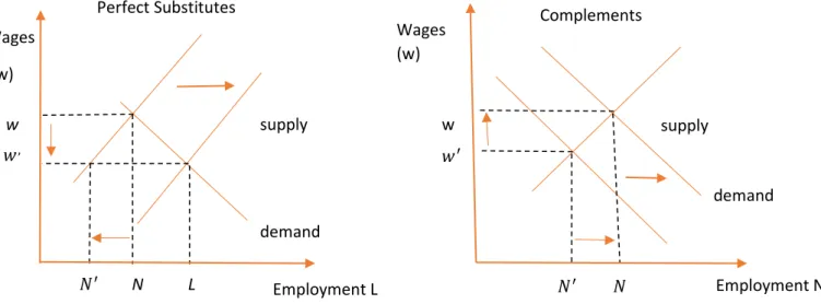
MMIGRATION

Let us now add the assumption that the workers are different according to their skill level. Workers can be skilled or unskilled and it applies to both natives and the immigrants. The immigrant workers can be perfect substitutes i.e. have the same skill set and occupation or they can be complements i.e. low skilled workers. If skilled immigrants are substitutes they will compete against each other for similar jobs. Therefore, in the short run the supply of skilled labour will increase due to which the supply curve will shift downwards, which shows a reduction in wages from w to 𝑤′and the total employment increases from N to L in the left panel of Figure 5. With the lower wage the number of native workers declines from N to 𝑁′ ,due to the positive slope of labor supply curve.

If the immigrants are complements, on the other hand, they do not compete with natives and belong to different markets. In this case, the native skilled workers can use their skills for

4_{This entire section of the theoretical background (Page 7–10) including figures builds on chapter 4 from the book} Labor Economics written by Borjas published in 2016.

demand supply Employment Wages P Q 𝐸∗ 𝑤∗

(15)

9

something better and the unskilled labor can do the work that does not require a high skill level. As immigrants and natives complement each other, the increase in the immigrants will increase the marginal product of natives, which will shift the demand curve to the right. This upward shift in the demand curve increases the demand for the high skilled natives. The increase in the productivity of natives will increase the wages of natives from 𝑤′ to w and native employment will also increase from 𝑁′to 𝑁, as can be seen in the panel to the right.

Figure 5: Immigration in short run perfect substitute & complements (Borjas,2016)

If immigrants and natives are perfect substitutes and capital is fixed, the wages of natives will be lower in the short run if the supply of immigrants is sufficient. However, it will raise the return to capital. This leads to more investments and thus higher marginal products of capital, which in turn pull wages upward (this is explained in the next section). If immigrants and natives are complements, then the wages of natives will be higher.

2.3 C

OBB

-D

OUGLAS

P

RODUCTION

F

UNCTION

To determine the production level, we will use a Cobb-Douglas production function. The production function shows how much output we can produce from given labor, technology and

demand demand w 𝑤, supply 𝑁′ N L 𝑁′ 𝑁 supply w 𝑤′ Employment L Employment N Wages (w) Wages (w)

(16)

10

capital. This Cobb-Douglas production function exhibits constant returns to scale, which means that an increase in both inputs by an equal amount will result in an equal increase in the output.

𝑄 = 𝐴𝐾𝑎_𝐿1−𝑎

Where Q is production, K is capital, L is labor, A is a constant and 𝑎 is a parameter that lies between 0 and 1.

According to marginal productivity theory, the factor of production is paid by the value of its marginal product. Assuming that, the price of Q is normalized to 1, this means that the labor is paid the real wage that is equal to the marginal product of labor and the price to capital is equal to the marginal product of capital (Borjas,2016).

𝑤 = 𝑀𝑃𝐿 = ⅆ𝑄 ⅆ𝐿 = (1 − 𝑎)𝐴𝐾 𝑎_𝐿−𝑎 𝑟 = 𝑀𝑃𝐾 = 𝑎𝐴 (𝐾 𝐿) 𝑎−1

Due to immigration the labor L increases, which increases the rate of return to capital and decreases the wage. However, in the long run firm invest in more capital which increases the capital K and thus wages and therefore people have more incentives to work.

(17)

11

3 METHODOLOGY

The two models that we have theoretically explained are by Altonji and Card (1991) and Borjas (1999), which includes immigrants and natives that have the same productivity and skill level (homogeneous labor) and also the case when they have different productivity and skill level (heterogeneous labor). In both cases, we will examine how the natives get benefit from immigration. The benefits of natives will be higher if there is more difference in the productivity and competence of immigrants. If immigrants and natives are complements, then natives will gain. If immigrants and natives compete against each other then natives will lose. Both models measure the change in wage level for native workers and the model by Borjas (1999) examines the total surplus, which also is explained in a graph.

3.1 H

OMOGENEOUS

L

ABOR

A

ND

I

NELASTIC

C

APITAL

We will here use the model of homogeneous labor and inelastic capital that Borjas (1999) has explained. This model will more stringently show the income of natives before and after immigration and the gain of native capitalist after immigration.

This analysis shows the effect of immigration on the labor market when immigrants and natives are perfect substitutes, which means that both share the same productivity and skill level. If immigrants and natives compete against each other for similar jobs, then in the short run natives will face a reduction in wages but the natives who own capital will gain.

We have a production function where K is the capital and L is the Labor, as before, but the function is now general.

𝑄 = 𝑓(𝐾, 𝐿)

The labor (L) consists of natives (N) and immigrant workers (M). The workers are perfect substitutes and L = N + M.

(18)

12

We start from a situation with no immigrant workers. The rental rate of capital when M = 0 is

𝑟0 = 𝑓𝑘(𝐾, 𝑁)

where the foot index k indicates the partial derivative with respect to capital. Similarly, the price of labor that is wage is

𝑤₀ = 𝑓_𝐿(𝐾, 𝑁)

The output from the production function is distributed to the native capitalists and the native workers, because the production function exhibits constant returns to scale.

3.1.1INCOME TO NATIVES BEFORE IMMIGRATION

The national income to natives before immigration is 𝑄_𝑁. 𝑄_𝑁= 𝑟₀𝐾 + 𝑤₀ 𝐿

The function 𝑓_𝐿 is the labor demand function. At given K the surface under this curve is the total income. To see this, note that

∫ 𝑓_𝐿(𝐾, 𝐿) ⅆ𝐿 𝑁 0 = [𝑓(𝐾, 𝑁)]₀𝑁 = 𝑓(𝐾, 𝑁) − 𝑓(𝐾, 0) = 𝑓(𝐾, 𝑁) = 𝑄_𝑁

The figure below illustrates the initial equilibrium. The capital is fixed and the area ABN0 is the national income

𝑄

_𝑁 to the natives. With the entry of immigrants, the supply curve shifts to the right and the wages fall from 𝑤₀ to 𝑤₁.

(19)

13 Figure 6: The immigration surplus in a model with homogeneous labor and fixed capital (Borjas,1999)

The area ACL0 is the new national income 𝑄₁. The part of the increase in the national income 𝑤1M is distributed to the immigrants. The area BCD is the immigration surplus and gives an increase in the national income. With immigration, the wages fall whereas the capital income

r increases (because 𝑓_𝐿𝐾 > 0). Immigration surplus is the portion that increases the return of capital and is the result of an increase in the supply of labor. Natives who own more capital will gain from the surplus and those who own less capital will primarily be affected by the lower wage.

3.1.2INCOME AFTER IMMIGRATION

With the entry of immigrants M, the rental rate of capital 𝑟₁ and the price of labor 𝑤₁is: 𝑟₁ = 𝑓_𝑘(𝐾, 𝐿)

𝑤₁ = 𝑓_𝐿(𝐾, 𝐿)

As mentioned above, income after immigration is the area ACL0 in Figure 6. Now the labor (L) consists of both natives (N) and immigrants (M).

𝑄₁ = 𝑟₁𝐾 + 𝑤₁𝐿

(20)

14

Because w₁ < w₀, native workers will be worse off because of fall in the wages. The native capital owners will be better off as the marginal product of capital gets higher when L increases. The net gain is BCD which is positive.

Let us now examine these welfare effects further. We know the wage 𝑤 = 𝑓_𝐿(𝐾, 𝐿) = 𝑓_𝐿(𝐾, 𝑁 + 𝑀). To find an expression for the net income gain we will take differential of wage with respect to immigration M.

ⅆ𝑤 =𝜕𝑓𝐿 𝜕𝐿 (𝐾, 𝑁 + 𝑀) ⅆ𝑀 ⅆ𝑤 =𝜕𝑓𝐿 𝜕𝐿 𝐿 𝑓_𝐿 𝑓_𝐿 𝐿ⅆ𝑀

Now define 𝜀 as the elasticity of factor price for labor (the percentage change in the wage resulting from a one percent change in the size of labor force), i.e. 𝜀 =𝜕𝑓𝐿

𝜕𝐿 𝐿 𝑓𝐿 = 𝜕𝑤 𝜕𝐿 𝐿 𝑤 The differential then is:

ⅆ𝑤 = 𝜀𝑓𝐿 𝐿ⅆ𝑀

3.1.3NET INCOME GAIN

The immigration surplus or the social net income gain BCD in the Figure 6 can be approximated by a triangle

𝛥𝑄_𝑁 = 1

2(𝑤0− 𝑤1)𝑀

Note that M is changing from 0 to M, so M = M – 0 = dM. Whereas (𝑤0− 𝑤1) = - 𝜕𝑤 𝜕𝐿 𝐿 𝑤𝑀 -dw = - 𝜀𝑓𝐿 𝐿 ⅆ𝑀 = -𝜀 𝑓𝐿

𝐿 𝑀. This means that

𝛥𝑄_𝑁 = − 1 2𝜀

𝑓_𝐿 𝐿𝑀𝑀

(21)

15

To simplify this, denote the income share of labor by 𝛼_𝐿 =𝑤𝐿 𝑄 =

𝑓𝐿𝐿

𝑄 and let m = 𝑀

𝐿 be the fraction of foreign-born in the labor force. The alternative expression for social net gain then is: 𝛥𝑄𝑁 𝑄 = − 1 2𝜀 𝑓_𝐿𝐿 𝑄 𝑀 𝐿 𝑀 𝐿

Using the definitions above the equation below shows that immigration surplus is proportional to the elasticity 𝜀. 𝛥𝑄𝑁 𝑄 = − 1 2𝜀𝛼𝐿𝑚 2

The equation above is an alternative expression for the social net income gain and it shows how much the country gains from immigration.

Borjas (1999) has used the numerical value of the share of labour income as 70%, the fraction of immigrants in the workforce slightly below 10% and the elasticity of factor price for labor around -0.3. Using these values in the above equation we get 0.1%. Which means the immigration surplus of US is 0.1% of GDP.

3.1.4NATIVE LABOR EARNINGS

After the immigration, income is redistributed from labor to capital. Due to immigration the area 𝑤0BD𝑤1 is lost by natives, as shown in the Figure 6.

The native labor earnings are

𝑤𝑁 = 𝑓𝐿(𝐾, 𝑁 + 𝑀)𝑁. We will take the differential with respect to M:

ⅆ(𝑤𝑁) =𝜕𝑓𝐿

𝜕𝐿 (𝐾, 𝑁 + 𝑀)𝑁ⅆ𝑀

As M is changing from 0 to M so we have M = M - 0 = ⅆ𝑀 = 𝑀 and defining 𝜀 =𝜕𝑓𝐿

𝜕𝐿 𝐿 𝑓𝐿 as

(22)

16 ⅆ(𝑤𝑁) =𝑓𝐿 𝐿 𝜕𝑓_𝐿 𝜕𝐿 𝐿 𝑓_𝐿𝑁 ⅆ𝑀 ⅆ(𝑤𝑁) =𝑓𝐿 𝐿 𝜀𝑁𝑀 ⅆ(𝑤𝑁) = 𝜀𝑓𝐿𝐿 1 𝑁 𝐿 𝑀 𝐿

As we know both natives and immigrants are in the labor market so L = N + M, we will solve for N, N = L-M. We will use N in the above equation and consider 𝑀

𝐿 = m to solve the equation further. ⅆ(𝑤𝑁) 𝑄 = 𝜀 𝑓𝐿𝐿 𝑄 (1 − 𝑚)𝑚 ⅆ(𝑤𝑁) 𝑄 = 𝜀𝛼𝐿(1 − 𝑚)𝑚

The equation shows the net change in the labor income of natives as a fraction of GDP Q. Using the same numerical values that Borjas (1999) has used that is 𝛼𝐿 = 0.7, 𝜀 = -0.3 and m = 0.1 in the equation above we get -1.9%. The minus sign shows a reduction in the wages which means that with the increase in the immigration the native labor earnings decreases by 1.9% of GDP.

3.1.5CAPITALISTS EARNINGS

The relative change of income to capital is obtained by subtracting the native labor earnings from the social net gain.

ⅆ(𝑟𝐾) 𝑄 = 𝛥𝑄_𝑁 𝑄 − ⅆ(𝑤𝑁) 𝑄 =1 2𝜀𝛼𝐿𝑚 2_{− 𝜀𝛼} 𝐿(1 − 𝑚)𝑚 ⅆ(𝑟𝐾) 𝑄 = −𝜀𝛼𝐿𝑚 (1 − 𝑚 2)

(23)

17

The equation above shows the net change in the income of capitalist as a fraction of GDP Q. The rectangle area 𝑤0BD𝑤1 and the immigration surplus BCD in Figure 6 goes to the native capitalists. Using the same values as above (𝛼𝐿 = 0.7, 𝜀 = -0.3 and m = 0.1) from the Borjas (1999) in the equation above we get 2% which means that the capital earnings of natives are about 2% of GDP. To sum up: While the net social gain is quite small, the redistribution is considerably larger.

For the implications of immigration in the case of heterogeneous labor we will use the next model of Altonji and Card (1991) because we think it is more suitable. The homogeneous model by Borjas (1999) looks at the economy in a big perspective, whereas the model by Altonji and Card (1991) looks at the economy at a smaller perspective which could be for example Stockholm or Västerås. We think it is interesting to look at both perspectives, hence we include a heterogeneous model into our paper as well.

3.2 H

ETEROGENEOUS

L

ABOR

This model is built on Altonji and Card (1991) where a municipal economy is distinguished locally. The economy produces a local good 𝑌 in a competitive industry, which is assumed to have CRS5. Inputs are unskilled and skilled labour, as well as other materials, such as capital and raw material. The output 𝑌 is then consumed locally within the economy and exported to other cities.

The total industry cost in the model is:

𝐶(𝑤_𝑠, 𝑤_𝑢, 𝑌) = 𝑌 ∙ 𝑐(𝑤_𝑠, 𝑤_𝑢)

Where the above equation measures the total industry cost as a function of the wages for unskilled and unskilled labor multiplied by the quantity of 𝑌. Let 𝑤_𝑠 and 𝑤_𝑢 denote the wage

(24)

18

levels for skilled workers and unskilled works respectively. By CRS, it is possible to pull out

Y, and thus c is the unit cost function.

3.2.1PRODUCT MARKET EQUILIBRIUM

Demand for the good 𝑌, arises from local demand from skilled workers, denoted as 𝑌_𝑠, local demand from unskilled workers, denoted as 𝑌𝑢, and export demand from the rest of the economy, denoted 𝑌𝑥. From this, we can form 3 demand functions, specified as per person demand, 𝐷𝑠(𝑞, 𝑤𝑠), 𝐷𝑢(𝑞, 𝑤𝑢) and 𝐷𝑥(𝑞). Which are demand for a skilled, unskilled and export respectively.

These are in turn used to form the following equation for the product market equilibrium: 𝑌 = 𝑃_𝑠∙ 𝐷_𝑠(𝑞, 𝑤_𝑠) + 𝑃_𝑢∙ 𝐷_𝑢(𝑞, 𝑤_𝑢) + 𝐷_𝑥(𝑞)

Let 𝑃_𝑠 and 𝑃_𝑢 denote the parts of the population in the economy that consist of skilled workers and unskilled workers, respectively. The last expression determining the market equilibrium is the demand for exportation.

For equilibrium in the labour market, the following requirement must be satisfied: (2𝑎) 𝑃𝑠∙ 𝐿𝑠(𝑤𝑠, 𝑞) = 𝑌 ∙ 𝑐1(𝑤𝑠, 𝑤𝑢)

(2𝑏) 𝑃𝑢∙ 𝐿𝑢(𝑤𝑠, 𝑞) = 𝑌 ∙ 𝑐2(𝑤𝑠, 𝑤𝑢)

The functions 𝑐1 and 𝑐2 denotes the partial derivative of the unit cost function with respect to unskilled and skilled wage rates respectively. Note that the RHS is the demand functions, which can be derived from the unit cost function.

3.2.2INFLOW OF IMMIGRANTS

Assume that we wish to analyse an inflow from immigrants and its effects. One of the elasticities used to analyse the model is:

(25)

19

𝜂_𝑖𝑗 = 𝜕𝑐𝑖 𝜕𝑤_𝑗

𝑤𝑗

𝑐_𝑖 , 𝑖 = 1,2 𝑗 = 𝑠, 𝑢.

This is the elasticity of labour demand for skill group 𝑖 with respect to the wage of group 𝑗. The elasticity of labor supply, 𝜀𝑖 of group 𝑖 is given by:

𝜀_𝑖 = 𝜕𝐿𝑖 𝜕𝑤_𝑖 𝑤𝑖 𝐿_𝑖 , 𝑖 = 𝑠, 𝑢. Let 𝛽 =𝑃𝑢 𝑃 and 𝛼 = 𝑃𝑠

𝑃, where β and 𝛼 denote the fractions of unskilled and skilled workers in the population respectively.

Let 𝜆_𝑠, 𝜆_𝑢 be numbers between 0 and 1 for the skilled and unskilled workers respectively, which can be determined with the following equations:

𝜆𝑢 = 𝑌 − 𝑌_𝑢− 𝑘₁∙ 𝑌_𝑠 𝑌 , 𝑘1 = 𝛽(1 − 𝛼) [𝛼(1 − 𝛽)]⁄ , 𝜆𝑠 = 𝑌 − 𝑘₂ ∙ 𝑌_𝑢− 𝑌_𝑠 𝑌 , 𝑘2 = 𝛽(1 − 𝛽) [𝛽(1 − 𝛼)]⁄ .

Finally, the stock of immigrants is denoted as 𝐼, so that the immigrant flow is given by ∆𝐼. Thus, the model above can be differentiated (see Appendix) to analyse the result from an inflow of immigrants. The differentiated system is formed as following:

(3a) 𝜆_𝑢(𝛼 𝛽⁄ ) Δ𝐼 𝑃⁄ = (𝜂_𝑢𝑢− 𝜀_𝑢)Δ log 𝑤_𝑢+ 𝜂_𝑢𝑠Δ 𝑙𝑜𝑔𝑤_𝑠

(3b) 𝜆_𝑠[(1 − 𝛼)(1 − 𝛽)] Δ𝐼 𝑃⁄ = 𝜂_𝑢𝑠Δ log 𝑤_𝑢 + (𝜂_𝑠𝑠 − 𝜀_𝑠)Δ log 𝑤_𝑠 The left-hand sides of the above equations measure the percentage increase in unskilled workers and skilled workers that results from an inflow of immigrants by Δ𝐼. The right-hand sides describe the changes in the wages of skilled and unskilled workers. To further understand these equations, note that 𝛼Δ𝐼 and (1 − 𝛼)Δ𝐼 are the changes in the portion of unskilled workers and skilled workers respectively. Thus, the proportional increases in the populations

(26)

20

of unskilled and skilled workers are given by, (𝛼 𝛽⁄ )Δ 𝐼 𝑃⁄ and [(1 − 𝛼)(1 − 𝛽)]∆𝐼/𝑃, respectively.

The model uses λ, as a factor to adjust for the gross increase in labor supply, for net increases in the demand, caused by immigrants. Furthermore, Altonji and Card (1991) gives a brief analyse that is dedicated especially to when the factor λ attains a specific value. The first case yields that, if immigrants possess the same skills as the natives, the following relationship will be true:

𝜆𝑢 = 𝜆𝑠 = 𝑌_𝑥

𝑌, Where 𝑌𝑥

𝑌, is the fraction of the good 𝑌 that is exported. This seems to be an accurate result, because this would mean that all labor force is equal and probably then give rise to some competition on the actual labor market.

On the other hand, if immigrants are less skilled than the natives, we have that,

𝜆_𝑢 > 𝑌𝑥 𝑌 > 𝜆𝑠.

This inequality is trustworthy since it shows exactly the relationship that is mentioned above and makes sense. It is also worth mentioning due to the previous statement, that Altonji and Card (1991), tells us that this relationship accentuates the effective increase in labor supply (newly arriving immigrants are considered as less skilled than natives).

Further investigation of the model determines that if the coefficient 𝜆 = 1, meaning that a 1 percentage increase of immigrants in the population (of the city) add nothing to the demand locally for produced output and decreases native wages by approximately 0.3-0.5 percent. Note that this is a finding by Altonji and Card (1991).

(27)

21

Let 𝑓 be the fraction of immigrants in the local population. If equations (3𝑎) and (3𝑏) are used, the model shows a relationship between the change in the wage rates, and the change in the fraction of immigrants:

∆𝑓 = ∆(𝐼 𝑃⁄ ) = (1 − 𝑓)Δ 𝐼 𝑃⁄ .

We note that when the demand for unskilled labor is not dependent of the wage rate for skilled labor, we have that:

𝜂_𝑢𝑠 = 0.

Equation (3𝑎) can be simplified to:

(4) Δ 𝑙𝑜𝑔 𝑤𝑢 = −𝜆𝑢

𝜀_𝑢−𝜂_𝑢𝑢(𝛼 𝛽⁄ ) Δ𝐼 𝑃⁄ = −𝜆𝑢

(1 − 𝑓)(𝜀 − 𝜂)(𝛼 𝛽)⁄ Δ𝑓

Equation (4) is originally built on Johnson (1980a), a special case where the notation 𝜆𝑢 here, is exactly equal to one and 𝛼 = 𝛽. Although, the above equation is built on the previously stated economist, this equation differs in two perspectives; namely, that it considers both unskilled and skilled workers, and the effect from demand of the good 𝑌.

However, if 𝜂𝑢𝑠 ≠ 0, the change in unskilled wage is:

(5) ∆ log 𝑤𝑢 = 𝐵𝑢 ∆ 𝐼 𝑃⁄ , Where,

𝐵_𝑢 =

−𝜆𝑢(𝛼 𝛽⁄ ) − 𝜆𝑠(1 − 𝛼)_{(1 − 𝛽)}𝜂𝑢𝑠⁄(𝜀𝑠− 𝜂𝑠𝑠) (𝜀_𝑢− 𝜂_𝑢𝑢) − 𝜂_𝑢𝑠𝜂_𝑠𝑢⁄(𝜀_𝑠 − 𝜂_𝑠𝑠) .

Recall that β and 𝛼 denote the fraction of unskilled and skilled workers in the population respectively. The above expression is a function of the supply and demand elasticities for

(28)

22

unskilled and skilled labor, respectively. The 𝜆_𝑠 denotes the fraction of 𝑌 that is exported to other cities.

Relating to the wage changes to immigrant inflows; suppose that 𝛼 = 𝛽, so that 𝜆𝑢 = 𝜆𝑠. Then, equation (5) can be rewritten as:

Δ log 𝑤_𝑢 = 𝜆𝑏_𝑢Δ 𝐼 𝑃⁄

Where the coefficient 𝑏_𝑢 for this case is negative. The value of 𝑏_𝑢 depends on how large in size the immigration inflow to a city is and also on the demand for the output of the good 𝑌. Furthermore, Altonji and Card (1991) suggest a result that; even if the parameters of the demand and supply is chosen widely, differently, the coefficient 𝑏_𝑢 will still be in the same interval between -0.49 up to -0.27, which suggests a relatively small interval difference. Moving to a most extreme case where the whole immigration inflow to the city will consist of unskilled labor, and the proportion of already existing skilled labor is equal to 0.5, the value of 𝑏_𝑢 then will be -2 up to -1. This means that the effect on the unskilled (already existing) labor’s wages will be as much as two to three times larger.

Also, worth mentioning is that another finding by Altonji and Card suggests that if labor supply is between zero and one, the reduction in per capita labor supply for natives will be between 0-0.5 percentages.

(29)

23

4 E

MPIRICAL

M

ODEL

This section includes a regression analysis, which will examine how unemployment is affected by immigration. The data that is used to perform the regression is mainly from Eurostat and the Swedish Migration Agency. The model includes two sets of data, where the first one (set 1) is from the period 1990-2017 and the second is from 2000-2017. Two sets of data are used, because in the second one immigration is divided into two categories, refugees and labor force, whereas in set 1 there is a lump of both, and the essence behind this is to see if the result will differ when the analysis includes both categories.

We have analyzed the data using excel and then discuss the results using some tables and explanation. The regression equation is an estimate of the change in unemployment explained by an inflow of immigrants and the growth rate of GDP in Sweden.

If you compare the growth in GDP between many countries, one can expect that it can be described by the change in unemployment ∆𝑢 over a time period, and the inflow of immigrants (𝐼𝑀) in a country. We would expect that unemployment will have a negative effect on the growth in GDP (𝑌), due to decreased spending and immigration to have a positive effect as a contradiction. To see this, we begin by looking at Okun’s law.

4.1 O

KUN

’

S

L

AW

Okun’s law is an empirical phenomenon, which was firstly studied by Arthur M. Okun. The Okun’s law shows a negative relationship between the unemployment and GDP6_{. It describes} how unemployment is related to growth in 𝑌, using the following regression equation:

∆𝑢𝑖 = 𝛽0+ 𝛽1𝑌𝑖 (1)

We would expect the signs to be 𝛽₀ > 0 and 𝛽₁ < 0. This is confirmed by the estimation.

(30)

24

4.2 E

STIMATION

Adding immigration to equation to (1), the equation becomes: ∆𝑢𝑖 = 𝛽0+ 𝛽1𝑌𝑖 + 𝛽2𝐼𝑀 (2)

Now, we turn to looking at the regression equation from data set 2, where immigration is consisting of both refugees and work permits. Again, we start with Okun’s law, where change in unemployment is described by the growth in 𝑌 and refugees (𝑅𝐸𝐹):

∆𝑢_𝑖 = 𝛽₀+ 𝛽₁𝑌_𝑖+ 𝛽₂𝑅𝐸𝐹_𝑖 (3)

Then we look at how the unemployment is explained by work permits (𝐿), and the equation instead becomes:

∆𝑢𝑖 = 𝛽0+ 𝛽1𝑌𝑖+ 𝛽2𝐿𝑖 (4)

Finally, we include both refugees and labor force into the regression equation: ∆𝑢_𝑖 = 𝛽₀+ 𝛽₁𝑌_𝑖 + 𝛽₂𝐿_𝑖+ 𝛽₃𝑅𝐸𝐹_𝑖 (5)

When change in unemployment is the dependent variable, the expected signs are: 𝛽₀ > 0, 𝛽₁ < 0, 𝛽2 < 0 and 𝛽3 < 0. The constant is expected to be greater than zero because if all other independent variables are zero, the change in unemployment will be positive. The negative sign of GDP is because unemployment and GDP are expected to have a negative correction to each other. If unemployment increases with some number, GDP is expected to decrease due to a fall in the purchasing power. The labor force (immigrants) consisting of refugees and work permits is expected to have a negative sign because the inflow of immigrants will increase the labor market and hence reduce unemployment.

(31)

25

4.3 R

ESULTS t-values in parentheses Regression equations Equation (𝟏) Equation (𝟐) Equation (𝟑) Equation (𝟒) Equation (𝟓) Intercept 0.008593 (4.373731611) 0.014208117 (3.726377513) 0.007262 (2.900992) 0.008494 (1.975887) 0.007545 (1.757134) GDP growth rate -0.30847 (-5.27048992) -0.316352532 (-5.59364663) -0.15864 (-2.79237) -0.1899 (-3.12509) -0.16075 (-2.49863) Refugees - - -1.47041 (-1.682140) - -1.41045 (-1.214327) Labor force - - - -2.38738 (--1.05137) -2.36422 (-0.083007) Immigration - -7.16145 (-1.69636446) - - - 𝐑𝟐 _0.536483 _0.588027341 _0.494082 _0.432239 _0.494372 𝐑̅𝟐 0.51717 0.552203632 0.416248 0.344891 0.367965

(32)

26

•REGRESSION RESULTS FROM EQUATION (1)

∆𝑢𝑖 = 𝛽0+ 𝛽1𝑌𝑖

We have started with equation (1) using Okun’s law where the dependent variable is change in unemployment rate and the independent variable is the growth rate of GDP.

The variables in equation (1) are in the expected direction. The negative sign of the GDP growth rate 𝑌, indicates that when here is a high growth in 𝑌 the unemployment in Sweden decreases. This is because if unemployment (𝑢) is low, people can spend more money on buying which would instead raise 𝑌. The intercept is quite close to zero, which means that if 𝑌 is equal to zero, the corresponding change in 𝑢 is almost zero as well. The t-values of the coefficients are high and significant and looking at 𝑅̅2_{, we can tell that the fit of the data to the} equation is quite okay. The t-values are quite high, so both the coefficients are significant here. •REGRESSION RESULTS FROM EQUATION (2)

∆𝑢_𝑖 = 𝛽₀ + 𝛽₁𝑌_𝑖+ 𝛽₂𝐼𝑀

In equation (2) we have added the immigration inflow (𝐼𝑀) in Okun’s law and it does not change the other coefficients substantially. Looking at 𝑅̅2_{, we note that adding immigration} raises the value significantly, which means that this variable has an explanation to the change in unemployment. Since the sign is negative, it means that unemployment is reduced by an immigration inflow to the labor market. The t-values are quite high, with 16 degrees of freedom. We can conclude that all the coefficients are significant.

∆𝑢_𝑖 = 𝛽₀+ 𝛽₁𝑌_𝑖 + 𝛽₂𝑅𝐸𝐹_𝑖

In equation (3) we have added the refugees to the regression equation. This raises 𝑅̅2 considerably, so the variable explains the unemployment well. Refugees seem to have a

(33)

27

negative effect on unemployment, which could be because refugees might join the labor force with the natives. As previously discussed, if immigrants that join the labor market have different skills than natives, it will be beneficial for everyone.

∆𝑢𝑖 = 𝛽0+ 𝛽1𝑌𝑖 + 𝛽2𝐿𝑖

In the equation (4) we have added the immigration inflow as labor force in the Okun’s law to see the how it effects the change in unemployment rate. The group of labor force seems to have an even stronger negative effect on the unemployment than refugees, which could be expected. Although the adding work permits instead of refugees seems to lower the 𝑅̅2, so the unemployment variable seems to be better explained if we only include refugees as a group.

One would have expected that the inflow of scarce competence should increase the marginal productivity of natives, and thus reduce unemployment. The t-values here are quite high as well, except the one for the labor force which is not significant.

∆𝑢𝑖 = 𝛽0+ 𝛽1𝑌𝑖+ 𝛽2𝐿𝑖 + 𝛽3𝑅𝐸𝐹𝑖

In the equation (5) we have refugees, labor force and the GDP growth rate as independent variables, describing the unemployment. We notice that the t-values gets too low to be significant. All the coefficients are still in the expected direction and the raise in R̅2_suggest that both the labor force and refugees describe unemployment in an efficient way (if we don’t consider the insignificance of the t-values). The problem with the low t-values suggests that there could be multicollinearity, which means that one or more of the independent variables is an imperfect linear combination of another independent variable.

(34)

28

5 SUMMARY AND CONCLUSION

This study shows that immigration can be beneficial for the economy in a country. If we recall the model by Borjas (1999) we can determine the wage level for natives after an inflow of immigrants into the labor market. Recall that this model assumes the natives and immigrants will possess the same skill level and thus compete with the same jobs. In the short run, natives will gain from capital they own as shown in figure 6, page 16, while native workers will lose.

To understand the results from the model by Altonji and Card (1991), we can look at the coefficient lambda, a percentage of how much immigrants add to the economy of a city, producing a local good. The model uses factors that will adjust the gross increases in the labor supply for net increases in the demand, caused by immigrants. If immigrants possess the same skills as the natives, the model tells us that the signs of lambda for unskilled workers, skilled workers and the fraction of the good 𝑌 that is exported all are equal to each other (i.e. have the same numerical value). If the lambda coefficient equals to the value of 1, this specifically means that a 1 percentage increase in the population of immigrants (for a city) adds nothing to the economy and we can see that in this case that immigrants reduce native wages, due to competition in the labor market. Also, this reduction of per capita labor supply is proportional to the reduction in wages (for natives and existing immigrants), multiplied by the elasticity for the labor supply. If the elasticity of the labor supply is between zero and one, it means that the decrease in native labor supply is between 0-0.5 percentages.

The empirical section of this study includes a regression analysis, where several regressions are run to see how change in unemployment rate can be explained by both immigration inflow and growth in the gross domestic product in Sweden. The result shows a negative correlation between both change in unemployment rate and gross domestic product, and with immigrants (refugees and work permits), so we can conclude that immigrants increase the labor force in Sweden into some extent. One would think that immigrants increase the unemployment due to

(35)

29

an increased competition on the labor market, but the empirical study suggests the contradiction.

The negative correlation between unemployment and gross domestic product in all five regression equations, suggests that immigration increase the economic growth in Sweden, due to an increase in purchasing power of products on the market.

Regression equation (5) includes immigrants divided into two groups (refugees and work permits). The result shows in-significance, looking at the t-values and comparing them with a critical value. It is hard to have significance in a multifactor regression model when the dependent is explained by many independent variable, since it can give arise for multicollinearity. But if we do not consider the low t-values, all the variables are in the expected direction as before and the raise in the value for 𝑅̅2, comparing with equation (5) tells us that all the independent variables explain the dependent variable in an efficient way.

This study suggests that immigration benefits both the economic growth and the labor market. However, it does not tell you how much it benefits the natives. An extended analysis could be done by investigating further to what extent and magnitude this affects a country.

(36)

30

REFERENCES

Altonji, J. and Card, D. (1991). The effects of immigration on the labor market outcomes of less-skilled natives. Immigration, Trade, and the Labor Market, pp.201 - 234.

Borjas, G. (1995). The Economic Benefits from Immigration. Journal of Economic

Perspectives, 9(2), pp.3-22.

Borjas, G. (1999). Labor Market Equilibrium. Handbook of labor economics. Volume 3. Amsterdam: North-Holland, pp.1697-1760.

Borjas, G. (2014). Immigration economics. 1st ed. Harvard University Press. Borjas, G. (2015). Labor economics. 7th ed. McGraw Hill Higher Education.

DN Fokus. (2018). Jennifer Hunt: ”Nästan alla vinner på invandringen”. [online] Available at: https://fokus.dn.se/jennifer-hunt-nastan-alla-vinner-pa-invandringen/ [Accessed 5 May 2018].

Ec.europa.eu. (2018). Eurostat. [online] Available at: http://ec.europa.eu/eurostat [Accessed 8 Apr. 2018].

Hunt, J. and Gauthier-Loiselle, M. (2010). How Much Does Immigration Boost Innovation?

American Economic Journal: Macroeconomics, 2(2), pp.31-56.

Mankiw, N. (2016). Macroeconomics. ed. New York, NY: Worth Publ. Migrationsverket. (2018). [online] Available at:

https://www.migrationsverket.se/download/18.2d998ffc151ac387159823b/1498556627690/R esidence%20permits%20granted%201980-2016.pdf [Accessed 3 May 2018].

Migrationsverket.se. (2018). Overview and time series. [online] Available at:

https://www.migrationsverket.se/English/About-the-Migration-Agency/Facts-and-statistics-/Statistics/Overview-and-time-series.html [Accessed 8 Jun. 2018].

Oxford Dictionaries | English. (n.d.). English Dictionary, Thesaurus, & grammar help |

Oxford Dictionaries. [online] Available at: https://en.oxforddictionaries.com [Accessed 8

May 2018].

Product, G. (n.d.). Sweden GDP - Gross Domestic Product. [online] countryeconomy.com. Available at: https://countryeconomy.com/gdp/sweden [Accessed 8 Apr. 2018].

Statistiska Centralbyrån. (2018). Immigration and emigration 1960−2016 and forecast

2017−2060. [online] Available at:

https://www.scb.se/en/finding-statistics/statistics-by- subject-area/population/population-projections/population-projections/pong/tables-and-graphs/the-future-population-of-sweden-20162060/immigration-and-emigration-and-forecast/ [Accessed 5 May 2018].

Statistiska Centralbyrån. (n.d.). Statistiska centralbyrån (SCB). [online] Available at: https://www.scb.se/ [Accessed 8 Jun. 2018].

(37)

31

APPENDIX

Table 1

Years Unemployment Rate GDP growth Immigrants Refugees Immigrants as Labor force 2000 2001 2002 2003 2004 2005 2006 2007 2008 2009 2010 2011 2012 2013 2014 2015 2016 2017 4.7 5.8 6 6.6 7.4 7.7 7.1 6.1 6.2 8.3 8.6 7.8 8 8 7.9 7.4 6.9 6.7 4.7 1.6 2.1 2.4 4.3 2.8 4.7 3.4 -0.6 -5.2 6 2.7 -0.3 1.2 2.6 4.1 3.2 2.4 10,546 7,941 8,493 6,460 6,140 8,859 25,096 18,414 11,237 11,265 12,130 12,726 17,405 28,998 35,642 36,645 71,571 31,685 15,759 12,809 10,135 10,249 8,529 5,985 6,257 9,859 14,513 17,954 16,373 17,877 19,936 19,292 15,872 16,975 24,709 32,294

(38)

32

Table 2

Years Unemployment Rate GDP growth Immigration inflow

1990 1991 1992 1993 1994 1995 1996 1997 1998 1999 2000 2001 2002 2003 2004 2005 2006 2007 2008 2009 2010 2011 2012 2013 2014 2015 2016 2017 1.65 2.96 5.53 8.25 7.96 7.71 8.05 8.03 6.48 5.58 4.7 5.8 6 6.6 7.4 7.7 7.1 6.1 6.2 8.3 8.6 7.8 8 8 7.9 7.4 6.9 6.7 0.8 -1 -1 -2 4.1 4 1.5 2.9 4.2 4.5 4.7 1.6 2.1 2.4 4.3 2.8 4.7 3.4 -0.6 -5.2 6 2.7 -0.3 1.2 2.6 4.1 3.2 2.4 37,120 41,948 34,602 58,769 78,860 32,296 31,390 36,132 39,070 37,033 60,490 56,872 54,396 56,787 58,811 62,463 86,436 86,095 90,021 98,644 91,458 93,134 111,090 116,587 110,610 109,235 150,535 130,556

(39)

33

MATHEMATICAL APPENDIX

Model by Card and Altonji (1991)

1. Product market equilibrium:

(1) 𝑌 = 𝑃_𝑠𝐷𝑠(𝑞, 𝑤𝑠) + 𝑃𝑢𝐷𝑢(𝑞, 𝑤𝑢) + 𝐷𝑥(𝑞)

2. Equilibrium in the local labor market:

(2𝑎) 𝐿_𝑠𝑃𝑠(𝑤𝑠, 𝑞) = 𝑌𝑐1(𝑤𝑠, 𝑤𝑢)

(2𝑏) 𝐿𝑢𝑃𝑢(𝑤𝑢, 𝑞) = 𝑌𝑐2(𝑤𝑠, 𝑤𝑢)

Assumptions:

Elasticity of labor demand for skill group 𝑖 with respect to the wage of group 𝑗

𝜂𝑖𝑗 = 𝜕𝑐_𝑖 𝜕𝑤_𝑗

𝑤_𝑗

𝑐_𝑖, 𝑖 = 1,2 𝑗 = 𝑠, 𝑢

Elasticity of labor supply, 𝜀𝑖 of group 𝑖

𝜀𝑖 = 𝜕𝐿𝑖 𝜕𝑤𝑖 𝑤𝑖 𝐿𝑖 , 𝑖 = 𝑠, 𝑢 The differential of (1): ⅆ𝑌 = 𝐷𝑠ⅆ𝑃𝑠+ 𝑃𝑠 𝜕𝐷𝑠 𝜕𝑞 ⅆ𝑞 + 𝐷𝑢ⅆ𝑃𝑢+ 𝑃𝑢 𝜕𝐷𝑢 𝜕𝑞 ⅆ𝑞 + 𝜕𝐷𝑧 𝜕𝑞 ⅆ𝑞 Collecting terms: (1′_{) ⅆ𝑌 = 𝐷} 𝑠ⅆ𝑃𝑠+ 𝐷𝑢ⅆ𝑃𝑢+ (𝑃𝑠 𝜕𝐷𝑠 𝜕𝑞 + 𝑃𝑢 𝜕𝐷𝑢 𝜕𝑞 + 𝜕𝐷𝑥 𝜕𝑞 ) ⅆ𝑞 Differential of (2a): 𝐿𝑠ⅆ𝑃𝑠+ 𝑃𝑠 𝜕𝐿𝑠 𝜕𝑤𝑠 ⅆ𝑤𝑠+ 𝑃𝑠 𝜕𝐿𝑠 𝜕𝑞 ⅆ𝑞 = 𝑐1ⅆ𝑌 + 𝑌 𝜕𝑐1 𝜕𝑤𝑠 ⅆ𝑤𝑠+ 𝑌 𝜕𝑐1 𝜕𝑤𝑢 ⅆ𝑤𝑢

(40)

34

Using the second part of the assumption (A1)

(2𝑎′) 𝐿𝑠ⅆ𝑃𝑠+ 𝑃𝑠 𝜕𝐿𝑠 𝜕𝑤𝑠 ⅆ𝑤𝑠= 𝑐1ⅆ𝑌 + 𝑌 𝜕𝑐1 𝜕𝑤𝑠 ⅆ𝑤𝑠+ 𝑌 𝜕𝑐1 𝜕𝑤𝑢 ⅆ𝑤𝑢 The differential of (2b): 𝐿𝑢ⅆ𝑃𝑢+ 𝑃𝑢 𝜕𝐿𝑢 𝜕𝑤𝑢 ⅆ𝑤𝑢+ 𝑃𝑢 𝜕𝐿𝑢 𝜕𝑞 ⅆ𝑞 = 𝑐2ⅆ𝑌 + 𝑌 𝜕𝑐2 𝜕𝑤𝑠 ⅆ𝑤𝑠+ 𝑌 𝜕𝑐2 𝜕𝑤𝑠 + 𝑌𝜕𝑐2 𝜕𝑤𝑢 ⅆ𝑤𝑢

Using the second part of the assumption (A1):

(2𝑏′_{) 𝐿} 𝑢ⅆ𝑃𝑢+ 𝑃𝑢 𝜕𝐿𝑢 𝜕𝑤𝑢 ⅆ𝑤𝑢= 𝑐2ⅆ𝑌 + 𝑌 𝜕𝑐2 𝜕𝑤𝑠 ⅆ𝑤𝑠+ 𝑌 𝜕𝑐2 𝜕𝑤𝑢 ⅆ𝑤𝑢

Assuming CRS and perfect competition, a function 𝑞, representing the unit price of the local output can be described as following:

𝑞 = 𝑐(𝑤𝑢, 𝑤𝑠), Which implies: ⅆ𝑞 = 𝜕𝑐 𝜕𝑤𝑠 ⅆ𝑤𝑠+ 𝜕𝑐 𝜕𝑤𝑢 ⅆ𝑤𝑢 ⅆ𝑞 𝑞 = 𝜕𝑐 𝜕𝑤𝑠 𝑤𝑠 𝑐 ∙ 𝜕𝑤𝑠 𝑤𝑠 + 𝜕𝑐 𝜕𝑤𝑢 𝑤𝑢 𝑐 ∙ ⅆ𝑤𝑢 𝑤𝑢 ⅆ𝑞 𝑞 = 𝜃𝑠 ⅆ𝑤𝑠 𝑤𝑠 + 𝜃𝑢 ⅆ𝑤𝑢 𝑤𝑢 ,

Where 𝜃𝑠 and 𝜃𝑢 is the share of the value of output that is paid as wages to skilled and unskilled workers, respectively.

Recall that 𝑃𝑠𝐿𝑠(𝑤𝑠, 𝑞) = 𝑌𝑐1(𝑤𝑠, 𝑤𝑢) and thus:

𝑐1=

𝑃𝑠𝐿𝑠

𝑌

(41)

35 𝑐1= 𝜕𝑐 𝜕𝑤𝑠 Substituting (1′₎_into_(2𝑎′₎_: 𝐿𝑠ⅆ𝑃𝑠+ 𝑃𝑠 𝜕𝐿𝑠 𝜕𝑤𝑠 ⅆ𝑤𝑠 = = 𝑐1[𝐷𝑠ⅆ𝑃𝑠+ 𝐷𝑢ⅆ𝑃𝑢+ (𝑃𝑠 𝜕𝐷𝑠 𝜕𝑞 + 𝑃𝑢 𝜕𝐷𝑢 𝜕𝑞 + 𝜕𝐷𝑥 𝜕𝑞 ) ⅆ𝑞] + 𝑌 𝜕𝑐1 𝜕𝑤𝑠 ⅆ𝑤𝑠+ 𝑌 𝜕𝑐1 𝜕𝑤𝑢 ⅆ𝑤𝑢 Eliminating 𝑑𝑞

𝑞 (and completing some elasticities):

𝐿𝑠ⅆ𝑃𝑠+ 𝑃𝑠𝐿𝑠 𝜕𝐿𝑠 𝜕𝑤𝑠 𝑤𝑠 𝐿𝑠 ∙ⅆ𝑤𝑠 𝑤𝑠 = = 𝑐1[𝐷𝑠ⅆ𝑃𝑠+ 𝐷𝑢ⅆ𝑃𝑢+ (𝑃𝑠 𝜕𝐷𝑠 𝜕𝑞 + 𝑃𝑢 𝜕𝐷𝑢 𝜕𝑞 + 𝜕𝐷𝑥 𝜕𝑞 ) 𝑞 (𝜃𝑠 ⅆ𝑤𝑠 𝑤𝑠 + 𝜃𝑢 ⅆ𝑤𝑢 𝑤𝑢 )] +𝑌𝑐1 𝜕𝑐1 𝜕𝑤𝑠 𝑤𝑠 𝑐1 ∙ⅆ𝑤𝑠 𝑤𝑠 + 𝑌𝑐1 𝜕𝑐1 𝜕𝑤𝑢 𝑤𝑢 𝑐1 ∙ⅆ𝑤𝑢 𝑤𝑢 Collecting terms: 𝐿𝑠ⅆ𝑃𝑠− 𝑐1𝐷𝑠ⅆ𝑃𝑠− 𝑐1𝐷𝑢ⅆ𝑃𝑢= = 𝑌𝑐1 𝜕𝑐1 𝜕𝑤𝑠 𝑤𝑠 𝑐1 ∙ⅆ𝑤𝑠 𝑤𝑠 + 𝑌𝑐1(𝑃𝑠 𝜕𝐷𝑠 𝜕𝑞 + 𝑃𝑢 𝜕𝐷𝑢 𝜕𝑞 + 𝜕𝐷𝑥 𝜕𝑞 ) 𝑞 𝑌(𝜃𝑠 ⅆ𝑤𝑠 𝑤𝑠 ) − 𝑃𝑠𝐿𝑠 𝜕𝐿𝑠 𝜕𝑤𝑠 𝑤𝑠 𝐿𝑠 ∙ⅆ𝑤𝑠 𝑤𝑠 + 𝑌𝑐1 𝜕𝑐1 𝜕𝑤𝑢 𝑤𝑢 𝑐1 ∙ⅆ𝑤𝑢 𝑤𝑢 + 𝑌𝑐1(𝑃𝑠 𝜕𝐷𝑠 𝜕𝑞 + 𝑃𝑢 𝜕𝐷𝑢 𝜕𝑞 + 𝜕𝐷𝑥 𝜕𝑞) 𝑞 𝑌(𝜃𝑢 ⅆ𝑤𝑢 𝑤𝑢 )

Using 𝑃𝑠𝐿𝑠= 𝑌𝑐1 and the definition:

𝛾 = (𝑃𝑠 𝜕𝐷𝑠 𝜕𝑞 + 𝑃𝑢 𝜕𝐷𝑢 𝜕𝑞 + 𝜕𝐷𝑥 𝜕𝑞 ) 𝑞 𝑌

Of the elasticity of demand with respect to q, we have:

𝐿𝑠ⅆ𝑃𝑠− 𝑐1𝐷𝑠ⅆ𝑃𝑠− 𝑐1𝐷𝑢ⅆ𝑃𝑢

𝑌𝑐1

(42)

36 𝜕𝑐1 𝜕𝑤𝑠 𝑤𝑠 𝑐1 ∙ⅆ𝑤𝑠 𝑤𝑠 + 𝛾 (𝜃𝑠 ⅆ𝑤𝑠 𝑤𝑠 ) −𝜕𝐿𝑠 𝜕𝑤𝑠 𝑤𝑠 𝐿𝑠 ∙ⅆ𝑤𝑠 𝑤𝑠 + 𝜕𝑐1 𝜕𝑤𝑢 𝑤𝑢 𝑐1 ∙ⅆ𝑤𝑢 𝑤𝑢 + 𝛾 (𝜃𝑢 ⅆ𝑤𝑢 𝑤𝑢 )

Rearranging and using the definition of 𝜀𝑠

𝐿𝑠ⅆ𝑃𝑠− 𝑐1𝐷𝑠ⅆ𝑃𝑠− 𝑐1𝐷𝑢ⅆ𝑃𝑢 𝑌𝑐1 = (𝜕𝑐1 𝜕𝑤𝑠 𝑤𝑠 𝑐1 + 𝛾𝜃𝑠− 𝜀𝑠) ⅆ𝑤𝑠 𝑤𝑠 + (𝜕𝑐1 𝜕𝑤𝑢 𝑤𝑢 𝑐1 + 𝛾𝜃𝑢) ⅆ𝑤𝑢 𝑤𝑢 Noting that 𝑑𝑤𝑠

The impact of immigration on the Swedish Economy

School of Business, Society & Engineering

Bachelor Thesis in Economics