Demonstration of the effects of harmonized speed on efficiency and traffic safety : A traffic simulation study of traffic interaction effects

VTInotat

Number: T 36 Date: 1988-07-29

Title: _{DEMONSTRATION OF THE EFFECTS OF HARMONIZED SPEED ON} EFFICIENCY AND TRAFFIC SAFETY

- A traffic simulation study of traffic interaction effects

Author: Arne Carlsson and Goran Nilsson

Division: Traffic Project: 813 00 02-2

Name: Prometheus PRO~NET Sponsor: Saab Scania

Statens vé'g och trafikinstitut

Vég:0",

Pa: 58101 Linkb'ping. Tel. 073-n5200. Telex50725 V7786! s

'IllStItlltBt

Besak: Olaus Magnus v59 37, Linképing

DEMONSTRATION OF THE EFFECTS OF

HARMONIZED SPEED ON EFFICIENCY AND TRAFFIC SAFETY - A traffic simulation study of

traffic interaction effects by Arne Carlsson and Goran NiIsson

PROMETHEUS PRONET

4.2 4.3

CONTENTS BACKGROUND PERFORMANCE

SOME IDEAS FROM THE STUDY RESULTS AND ANALYSIS

Traffic characteristics at free flow condition

Traffic interaction effects at the traffic volume 750 vehicles/hour

Traffic effects with lorries and buses excluded

Appendix: Figures.

1 BACKGROUND

Speed and speed behaviour are the two basic factors for efficiency and safety in road traffic.

As variations in speed have negative effects both on efficiency and safety it is important to demonstrate the benefits due to reduced speed

variation.

One fundamental question is which factors contribute to the speed variation. From the knowledge that drivers are well aware of their speed level, the following hypothesis can be formulated.

Different drivers and drivers in different situations make varying choices of speed level, based on the speed limit and/or the speed shown on the speedometer.

This means that on a road where the speed limit is low in relation to the standard of the road, vehicles ought to be concentrated very closely to the speed limit. However, this is not the case. The speed distribution is normally more or less continuous with a large variation (discrete speed values cannot be isolated).

In a limited study on the inaccuracy of speedometers, it was found that the negative bias of speedometers was in the range of 0-12 km/ h.

According to the hypothesis above these results still pose the question of whether drivers choose discrete speed levels due to the speed limit and the speedometer, but the inaccuracy of the speedometers results in a continuous spectra of speed.

In order to test these assumptions the VTI traffic simulation model has

2 PERFORMANCE

The test road was a two-lane road with a road width of 9 meters and a length of 12 km. The speed limit was 90 km/h and the traffic volume 750 vehicles/ h in both directions. 12 % of the vehicles were lorries and buses. Traffic simulation I

The passenger cars were clustered into 5 speed levels, 80, 90, 100, 110 and 120 km/h and the lorries were clustered into 3 speed levels 80, 90 and ICC km/h. This choice of speed level was calculated in order to achieve the same journey speed and standard deviation in speed, as was known from empirical data.

Two different simulations were performed one with accurate speedo-meters and one with inaccurate speedospeedo-meters. The inaccuracy of the speedometers was minus 5 km/ h with a standard deviation of 2 km/h. Traffic simulation 11

In another pair of traffic simulations, with and without accurate speedo-meters, three speed levels were chosen for passenger cars viz. 90, 100 and 110 km/h and four speed levels for lorries viz. 80, 85, 90 and 95 km/h. Two ideal situations are available. One traffic situation represents only one speed level with accurate speedometers - speed level 95 km/h. The other traffic situation represents only one speed level with inaccurate speedometers - speed level 90 km/ h with a standard deviation of 2 km/h. Traffic simulation III

In a third simulation study the lorries were excluded from the second traffic simulation which means three speed levels viz. 90, 100 and 110 km/h. This was made in two different ways. In the first case the lorries were just excluded which means that the traffic volume decreased to 660 vehicles/h. In the second case the lorries were replaced with passenger cars in order to keep the vehicle flow unchanged. The traffic simulations were performed with and without accurate speedometers.

3 SOME IDEAS FROM THE STUDY

Before the detailed presentation of the results is given, it might be of some value to present ideas which are based on the results.

The idea of a total harmony of speeds, according to road and traffic conditions, into one speed level is perhaps unrealistic but the current speed limit systems are partly based on that idea.

The observance of speed limits shows that some people drive slower than speed limit and some drive faster. A small group drives much faster. The size of this latter group depends on the enforcement acitivities and the level of the speed limit.

Accurate speedometers can result in speeds being clustered to discrete speed levels, for example the speed limit, 10 km/h over the speed limit etc.

Assume that vehicles are equipped with speed cruise controls with the possibility for the driver to choose three different speed levels d-low, normal or fast. The values of these three speed levels are given automatically depending on the road and traffic situation. The differences between these three speed levels can be different and do not need to correspond to lOth's of kilometers. This will give a speed limit system with alternatives for the drivers. Multilane roads can have different speed

4 RESULTS AND ANALYSIS

4-.1 Traffic characteristics at free flow condition

To make meaningful comparisons of interaction effects in traffic, the characteristics at free flow conditions must be the same in adequate measures. In our case the free flow speedsare the same for different

traffic conditions.

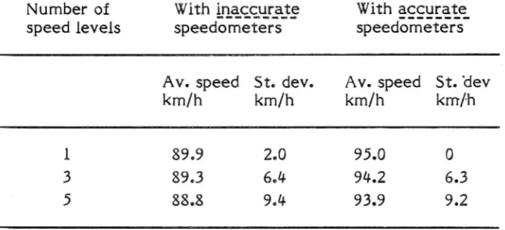
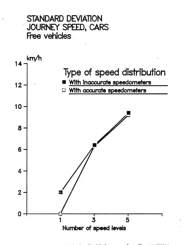
Table No. 1 below shows the average journey speed and standard deviation of cars in the simulated traffic conditions at free flow condition. The different traffic conditions are described in chapter 2.

Table 1. Average journey speed (km/h) of cars and standard deviation of different traffics. Free flow condition.

Number of With inaccurate With accurate

speed levels speedometers speedometers Av. speed St. dev. Av. speed St. 'dev km/h km/h km/h km/h

1 89.9 2.0 95.0 0

3 89.3 6.4 94.2 6.3

5 88.8 9.4!- 93.9 9.2

The first line of the table (one speed level) is the ideal situation. The difference in journey speed is 5 km/h between accurate and inaccurate speedometers.

The greatest influence on the standard deviation comes from the number of speed levels. The "internal" variation inside every speed level has very little influence on the standard deviation.

It may be noted that the traffic with 5 speed levels and inaccurate speedometers is very close to normal Swedish traffic on roads with a 90 km/h speed limit. (The normal free flow value of cars are 89.5 and 9.3 km/h in st. deviation).

The slight decrease in average journey speed with the number of speed levels is a result of increasing standard deviation, in speeds.

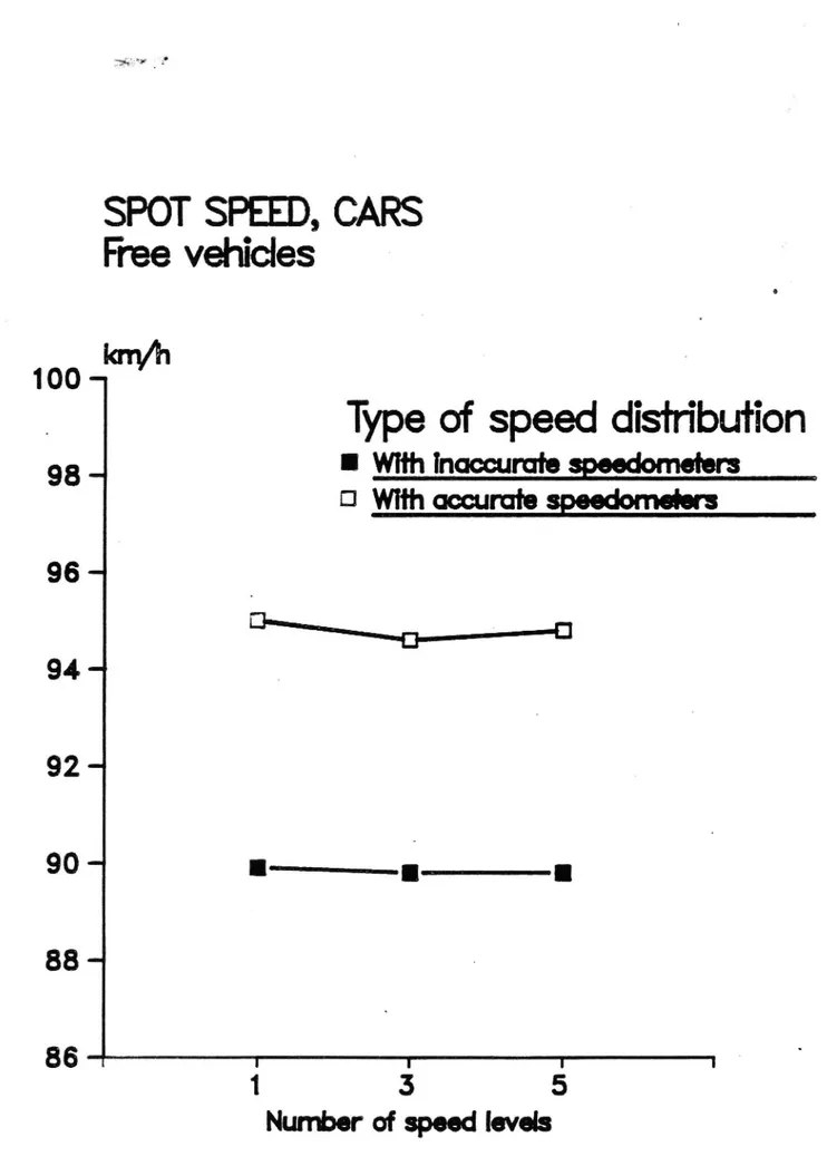
In the next table, the average spot speed of cars in the middle of the simulated section are presented. The average spot speed is measured as time mean speed for cars at free flow.

Table 2. Average spot speed of cars and standard deviation in the middle of the section. Time mean speed at free flow condition.

Number of With inaggugantq With accurate speed levels speedometers speedometers

Av. speed St. dev. Av. speed St. dev km/h km/h km/h km/h

1 89.9 2.0 95.0 0

3 89.8 6.6 94.6 6.6

5 89.8 9.5 94.8 9.4

There are only very small differences in average spot speeds between the different traffic conditions, with exception of the 5 km/h difference in speed according to the speedometers.

Table l and 2 are illustrated in figures 1 3 in the appendix.

In the traffic conditions with 3 and 5 speed levels there are 12 % of lorries or buses. The average journey speed for these vehicles is 79 km/h and 84.4 km/h respectively which implies an average of'lO km/ h below the average of cars.

We can summarize that all the different traffic conditions have the same average speeds, with the exception of 5 km/h depending on the speedo-meters. The standard deviation in the speed distribution depends almost totally on the numbers of speed levels.

4.2 Traffic interaction effects at the traffic volume

750 vehicles/ hour

The effect of clustering the vehicles into different numbers of speed

levels was studied at a traffic volume of 750 vehicles/hour in both direction.

Table 3 shows the average journey speed of cars at this flow.

Table 3. Average journey speed of cars at traffic volume 750 vehicles/hour

Number of With inaccurate With accurate speed levels speedometers speedometers

Av. speed Av. speed

km/ h km/h

1 89.1 95.0

3 83.3 . 88.7

5 79.8 i - 86.1

A rapid decrease in journey speed can be observed, when the number of speed levels is increased. On the other hand the internal variation in speed at each level has just a small influence. The difference in speed is just about 6 km/h between accurate and inaccurate speedometers.

Figure 4 illustrates the speed-flow diagram for the different cases. The slope of the curves varies to a great extent with the number of speed

levels.

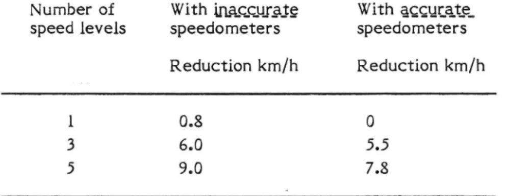
A more detailed analysis is made in table 4. It shows the reduction in journey speed, i.e. difference in average speed between free flow conditon and 750 vehicles/hour. This reduction is purely an effect of the number of speed levels and standard deviation in speed.

Table 4. Reduction in journey speed of cars at 750 vehicles/hour

Number of With Ln_a_c_c_u_r_a_t§ With accurate speed levels speedometers speedometers

Reduction km/h Reduction km/ h

l 0.8 0

3 6.0 5.5

5 9.0 7.8

The reduction in journey speed is increasing rapidly, when the number of speed levels is increasing. But the internal variation on each speed level causes just a delay of about 1 km/h extra. The table above is illustrated in figure 5.

Which are the reasons for the higher journey speeds, when clustering the vehicle in speed levels?

The explanation is fewer catching-ups and shorter platoon lengths. To prove these facts some traffic interaction effects have been investigated. Tabel 5 shows the overtaking rates for cars at 750 vehicles/hour. The overtaking rate is measured as the average number of overtakings performed per vehicle and vehicle kilometre.

Table 5. Overtaking rates of cars at 750 vehicles/ hour Number of With i_n_a_c_c_u__r_a_t§ With aggugate speed levels speedometers speedometers

Ovt. rate Ovt. rate

1 0.062 0

3 0.108 0.071

Again we can observe a very strong influence due to the number of speed levels. The overtaking rate increases with several speed levels. In this case there is also an influence from the internal speed variation. There is an obvious difference between accurate and inaccurate speedometers. This can be observed veryclearly in figure 6, showing the overtaking rate. We have the same pattern as above for the proportion of constrained journey time for all vehicles. This effect is very sensitive to the

catching-up frequency. ,4

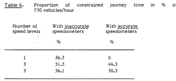
Table 6 gives the proportion of constrained journey time. Notice that it is the constrained time for all vehicles, also lorries and buses.

Table 6. Proportion of constrained journey time in % at 750 vehicles/hour

Number of With inaggugate With agcugate speed levels speedometers speedOmeters

_ % %

1 36.3 O

51.5 44.3

5 56.1 50.5

Again there are two influences. A strong one, deplending of number of speed levels, and a weaker one, depending on the internal speed variation inside very speed level. Figure 7 illustrates this.

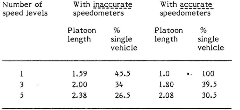
The proportion of constrained journey time is very strongly connected with the average platoon length. When the platoons are growing the constrained journey time will increase. Table 7 shows the average platoon length together with the proportion of single vehicles. A single vehicle has no other vehicle either in front or in the back within a time gap of 3

Table 7. Average platoon length and proportion of a single vehicle at 750 vehicles/hour

Number of

With tracers}?

With assgzeté

speed levels speedometers speedometers Platoon % Platoon % length single length single

vehicle vehicle

1 1.59 45.5 1.0 m 100

3 . 2.00 34 1.80 39.5

5 2.38 26.5 2.08 30.5

The results follow the same pattern as the other interaction effects. One very strong influence from the number of speed levels and one weak influence from the internal variation, depending on the inaccuracy of the speedometer. The results above are illustrated in figure 8 and 9 in appendix. One can notice that clustering the speed of the vehicles will result in much more single vehicles in the traffic, which can be regarded as improved comfort in traffic.

The results can in short be summarized as follows. Very great improve-ment in efficiency and safety in road traffic can be achieved by clustering the vehicles in speed levels. But also accurate speedometers will give effects by reducing platoon lengths and overtaking rates.

4.3 Traffic effects with lorries and buses excluded

In the preceding chapter, the traffic conditions with 3 and 5 speed levels include lorries and buses. The average journey speed for these vehicles is 10 km/h below that for cars. Even .if the proportion just is 12 %, one can

assume that the cars will be constrained.

In order to investigate the influence of these vehicles simulations have been performed with lorries and buses excluded.

10

The traffic conditions chosen were three speed levels for cars and excluding the heavy vehicles in two different ways. In the first case the heavy vehicles were replaced with cars in order to keep the traffic volume constant. This gives the opportunity to isolate the influence of lorries and buses. In the second case these vehicles were simply excluded, and this will also give the effects of decreasing the traffic volume with 12 0/0.

Table 8 below gives the results for journey. speed in the different cases. Table 8. Journey speed (km/h) for cars at different vehicle

compo-sitions. 3 speed levels forcars. Vehicle composition

Type of Cars and just cars just cars speedometers lorries 12 % 750 vehicles/h 660 vehicles/h

750 vehicles/h

{Qaggurafe 83.3 86.0 86.5 Accurate 88.7 91.1; 91.8

The absence of lorries and buses results in a considerable increase in journey speed for cars. The reason is that fewer cars are constrained (i.e. these that previously were constrained by heavy vehicles). Consequently the standard deviation is less in a traffic population only consisting of cars. With three speed levels for cars the total standard deviation decreased from 6.8 to 6.3 km/h.

The additional increase in journey speed, when the traffic volume decreases 12 % with the absence of lorries, is small.

Figure 10 illustrates the speed-flow diagram of all four cases. The slope of the speed curve gives the influence of heavy vehicles when present and

absent.

Again the explanations for higher journey speed are fewer catching-ups and shorter platoon lengths.

11

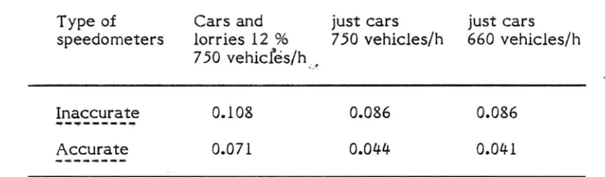
Table 9 below shows the overtaking rates for cars in the different cases.

Table 9. Overtaking rates (ovt/carkm) for cars at different vehicle compositions. 3 speed levels for cars.

Vehicle composition

Type of Cars and just cars just cars speedometers lorries 12 0/0 750 vehicles/h 660 vehicles/h

750 vehiclae's/hd

inaccurate

0.108

0.086

0.086

Accurate 0.071 0.044 0.041

There is a decrease in overtaking rate of 20 % with inaccurate speedo-meters and 4O % with accurate speedospeedo-meters when excluding the lorries. This is a result of fewer catching-ups when the slow-moving lorries have been excluded. it should be noticed, that in traffic with both cars and lorries involved, 30 % and 40 % of the overtakings, respectively, are overtakings between car and lorry, although the proportion of lorries is just 12 %.

The influence of the decreasing traffic volume is almost insignificant in this respect.

If we look upon the proportion of constrained journey time, there is almost the same pattern.

12

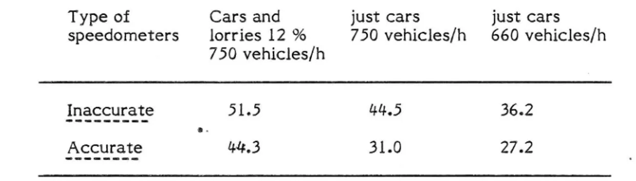
Table 10. Proportion of constrained journey time in %, at different vehicle compositions. 3 speed levels for cars.

Vehicle composition

Type of Cars and just cars just cars speedometers lorries 12 % 750 vehicles/h 660 vehicles/h

750 vehicles/h

Inaccurate 51.5 4&5 36.2 Accurate ##.3 31.0 27.2

There is a significant reduction in constrained journey time, when excluding the lorries. The presence of lorries will cause more catching-o ups and longer platoons, because of their lower speed.

The decrease in traffic volume also has an effect in this respect. The constrained journey time will be reduced when the flow is decreased. Table 9 and 10 are illustrated in figures ll and 12. The presence and absence of lorries is clearly observable.

The results can be summerized in the following way. When clustering the vehicle in different speed classes, there are great benefits to achieve if the heavy vehicles have the same levels as cars. The efficiency will increase if the speed difference between cars and lorries can be reduced.

Appendix

JOURNEY SPEED, CARS

Free vehicles

100

-Type of speed dlmbmaon

98 ..

I With haccurafe speedome er

D With accurate speedometer

925 ._

94 a

\

g

92 a

[\88

-as

.

r

r

i

1

3

5

STANDARD DEVIATION

' JOURNEY SPEED, CARS

Free vehicles .

14 -km/h

Type of speed disiribuiion

12 _ -

I With inaccurate speedometer:

E1 With accum re speedometers

10

-I

2 ..

₁

₃

₅

Number of speed levcis

SPOT SPEED, CARS

Free vehicles

100

-Type of speed distribution

98 _

With inaccurate speedometer:

C! With accurate speedometer:

96 -

o

D

+

A:

94

92

-9° "

l

a

I

88

-86

r

r

I

u

1

3

5

Number of speed levels

JOURNEY SPEED, CARS

Type of speed distribution

I W M

96 km/h

_{U macaw 29-30mm}

-i _ _

-

-

_{- -E1 ispeed level}

ispoodlwd

"' Sspeedbvels

5 speed levels

3 speed levels

I Sspeedlevels

7e

. ,

r

I

I

0

250

500

750

1000

Traf c voluma

RDUCTlON IN JOURNEY SPEED. CARS

Traffic volume : 750 veh/h

km/h

14-Type of speed distribution

12_

_{Wifhinaowrafespoodomohrs}

,

_{Withacwrafe speedometer:}

.10-I

4..

O

_H

_'

_'

_'

1

3

5

Nun'berofspeedlovels

OVERTAKING RATE, CARS

Traf c volume : 750 veWh

. 14 3me

I

. 12 -

/

I

. 1o

-

.08-.06-

'

_{Il\MM1hmawm napaukmumus}

Type of speed disfribu on

FIWthnaumbapaukmumrs

.oo

, .r

,

r

1

3

5

anmerofqpauikmds

Tinf c volume : 750 van/h

%

70

-60 ->

aff " " ll

so -

"

4o

-I

30

-20 -

-Type of speed disiribuiion

1O _.

I With inaccurate speedometer:

C1 With accurate sp'eedomefers

O H4 r I l

1

3

5

Number of speed levels

AVERAGE PLATOON LENGHT

Traffic volume : 750 veh/h

No. of veh

2 . 5

-2 .

1 . 5

-1' -

_{Type of speed distribution}

I With inaccurate speedomem ers

O 5

_{C] With accurate speedomefers}

O

_u

_I

_'

_I

₇

1

. 3

5

Number of speed levels

PROPORTION OF SINGLE VEHICLES

Traffic volume : 750 veh/h

Type of speed distribution

90 -

_{I With inaccurate speedometer:}

El With commie speedometers

70-

60-

50-40

3020

-10

1

~ 3.

5

Number of speed levels

JOURNEY SPEED, CARS

I 3 speed levels

Type of speed distribution

3

km/h

_{mammmg mossorgmg a; s}

80

-78 I . T l |

0

250

500

750

1000

Traf c volume (veh/h)

.Eigg[g_lg Speed-flow diagram for cars in different compositions. 3 speed levels for cars.

OVERTAKING RATE, CARS

3 speed levels

Type of speed distribution

0

_I

_{Inaccurate 13%;...}

o 14 wooden

, D mew-1! MM-

'0 . 12

-I Lorries

0 . 10

'-Qma >30 tomes

0 . 08

-ll] Lorries

0 . 06

-t?

_{531'2 3-9:}

0 . 04

0 . 02

-0.00 3"

_I

_'

_I

_l

I

o

₂₅₀

₅₀₀

₇₅₀

₁₀₀₀

Traf c volume (Veh/h)

Eigggg_ll Overtaking rate for cars in different veh1c1e compositions. 3 soeed 1eve1s for raw:

PROPORTION OF CONSTRAINED JOURNEY TIME

3 speed levels

a

%

70-

60-50

40-

30-Type of speed distribution

35

level;

Cl mamgmg tend. Icy-be.

I

Lorries

{1,13 Lorries

/

_{. //}

4/

/ E: No Sorriw

l

. l

l

250

500

750

1000

Traf c volume (van/h)

Proportion Of constrained journey time in different vehicle compositions. 3 speed ieveis for cars.