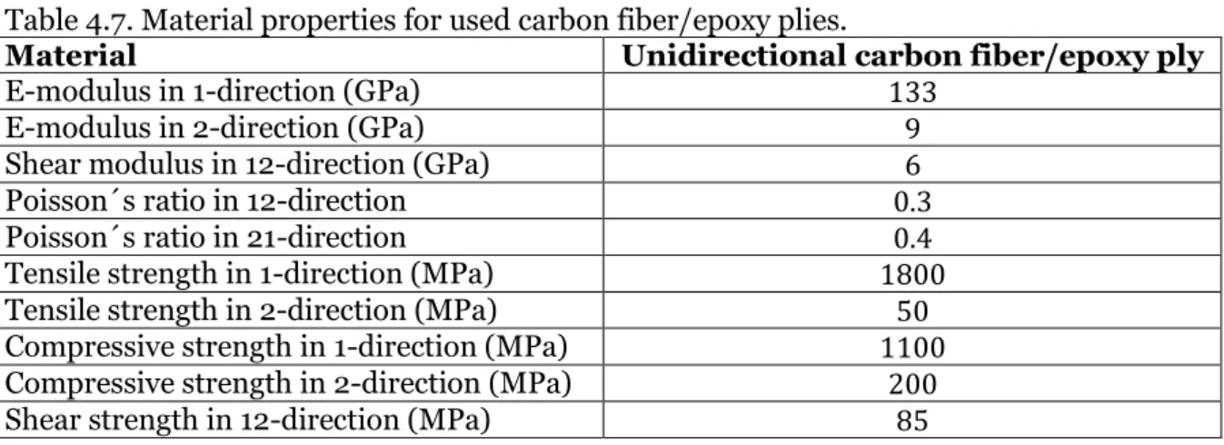
Development of composite fin to Improved Orion rocket.

(1)

Author: Petter Ekman Report code: MDH.IDT.FLYG.datum.GN300.15HP.Ae

Development of composite

fin to improved Orion rocket

BACHELOR THESIS IN

AERONAUTICAL ENGINEERING

15 CREDITS BASIC LEVEL 300

(2)

(3)

i

Abstract

Today Swedish Space Corporation use sounding rockets and high-altitude balloons for making different measurements and experiments in the atmosphere. The launches are made from ESRANGE in Kiruna, Sweden. REXUS/BEXUS is an international collaboration between universities and the Swedish and German Space board.

The rockets used today can be one or two stage engine rockets that can reach heights of over 100 km over the sea level. The rocket engines are used only a short time under the launch and then the rocket “glides” the remaining distance. During the launch the rocket accelerate about 24 g and reach a speed of 5.5 times the speed of sound. This places great demands on the fins structure.

The rocket fins used today are made of aluminum and have a leading edge made of steel. The fins are originally designed by NASA a long time ago. By reducing the weight of the fin either more payloads can be carried or less fuel may be consumed.

The main objective of this thesis was to evaluate if it is possible to construct a composite based fin that is lighter, equally stiff and still able to withstand the structural stresses. The idea was that by using CAD (Computer Aided Design), CLT (Classical laminate Theory) and FEM (Finite Element Method) as tools, structural forces can be evaluated and the new structure be optimized. As basis there was an old used fin and CAD-geometry of a newer variant of the fin. By estimating the loads acting on the fin from flight data and from the geometry of the current fin, ultimate stresses of the new developed composite based fin can be estimated.

The advantage by using composite materials instead of metals is that they are considerably lighter, but still has the same or even better stiffness and strength. By placing the composite’s fibers in different directions the strength and stiffness can be controlled for the component. To increase the bending stiffness, but without increasing the weight much, a core can be put between two laminates and thereby create a sandwich structure. In the aerospace industry this construction form is widely used.

The future of this project needs to include analysis of vibrations and the connection between the fin and fuselage of the rocket. A more complex analysis of the loads and especially the thermal loads acting on the fin should also be considered.

(4)

ii

Sammanfattning

Idag använder Svenska Rymdstyrelsen höghöjdsraketer och höghöjdsballonger för att göra olika mätningar och experiment i atmosfären. Uppskjutningarna görs från ESRANGE i Kiruna. REXUS/BEXUS är ett internationellt samarbete mellan universitet, Svenska Rymdstyrelsen och den tyska rymdstyrelsen.

Raketerna som används idag består av en- eller flerstegsraketer som kan nå höjder upp emot 100 km över havet. Raketens motorer används bara en kort stund under uppskjutningen, resterande bit kommer raketen glidflyga. Under uppskjutningen utsätts raketen för

accelerationer runt 24 g och når hastigheter runt 5,5 gånger ljudets hastighet. Detta ställer höga krav på fenans struktur.

Fenorna som används idag är byggda av aluminium med en stålframkant. De designades av NASA för en längre tid sedan. Genom att reducera vikten på fenan kan mera nyttolast bäras eller mindre bränsle användas.

Huvudsyftet med detta examensarbete var att undersöka och utveckla en kompositbaserad fena som är lättare och kan stå emot de krafter som fenan utsätts för under uppskjutningen. Genom att använda program som CAD (datorstödd modellering), CLT (klassisk laminatteori) och FEM (finita elementmetoden) som verktyg kunde de strukturella krafterna bestämmas och den nya strukturen optimeras. Som underlag användes en äldre använd fena och CAD-geometri för en nyare variant av fenan. Genom att bestämma de krafter som nuvarande fenan utsätts för från flygdata, kunde de maximala krafterna bestämmas, och den nya fenan kunde klara av samma belastningar.

Fördelen med att använda kompositmaterial istället för metaller är att de är betydligt lättare och har samma eller till och med högre styrka och styvhet. Genom att lägga fibrerna i olika riktningar kan därmed styrka och styvhet styras hos komponenten. Genom att använda ett lätt distansmaterial mellan två kompositlaminat kan böjstyvheten ökas kraftigt, med endast en marginell viktökning till följd. Inom flyg och rymdindustrin används ofta denna

konstruktionsmetod.

Framtida arbete kring denna fena behöver analyser av vibrationer, infästning och de termiska lasterna.

(5)

iii

Date: 19 September 2012

Carried out for: SSC Space

Supervisor: Erik Marklund

Ph.D. Researcher Composite Structures Swerea SICOMP AB

Email: erik.marklund@swerea.se Advisor at SSC Space: Olle Persson

Manager Fight Safety & Operation Sounding Rockets & Balloons SSC Esrange

Email: olle.persson@sscspace.com Examinator: Per Schlund

Lecturer in Aeronautical Engineering

School of Innovation, Design and Engineering Mälardalen University

(6)

iv

Acknowledgements

I would like to thank Erik Marklund for all the help under this thesis. Without all the help and hints this thesis could not been carried out in a proper way.

(7)

1

Symbols and Subscripts

A Area

Cross-sectional area of the fiber Cross-sectional area of the matrix Drag coefficient

Drag

Fiber elastic modulus Elastic modulus in L-direction Matrix elastic modulus Elastic modulus in T-direction Force vector

Tsai-Wu constant (i=1,2,6 and j=1,2,6) Shear modulus in LT-plane

Shear modulus of the matrix Height

Structural stiffness Ply index

L Longitudinal

Moment in ij-direction (i=x,y and j=x,y) Force in ij-direction (i=x,y and j=x,y)

Force in L-direction Force carried by fiber Force carried by matrix Force in T-direction Dynamic pressure T Transverse Fiber thickness Matrix thickness Thickness in T-direction Fiber volume fraction Matrix volume fraction Displacement vector

Coefficient of thermal expansion

Shear strain in xy-plane

Longitudinal displacement of the fiber Longitudinal displacement of the matrix Longitudinal displacement of the composite Transverse displacement of the fiber Transverse displacement of the matrix Transverse displacement of the composite Strain of the fiber

Strain in L-direction

Longitudinal strain of the fiber Longitudinal strain of the matrix Strain of the matrix

Strain in T-direction Transverse strain of the fiber Transverse of the matrix Halpin-Tsai constant Degrees

Poisson´s ratio in LT-plane

Halpin-Tsai parameter Composite density Fiber density Matrix density Stress in fiber

Stress in ij direction (i=0,1,2,6 and j=1,2,6)

Stress in L-direction Stress in matrix Stress in T-direction

(11)

5

1. Introduction

1.1 Background

SSC was founded as Svenska Rymdaktiebolaget by the Swedish government in 1972 to be the executive of the National Delegation of Space Activities (today Swedish National Space Board). SSC has its roots from ESRANGE Space and Technology Group in Solna. 1972 ESRANGE went from being a European facility to a full Swedish own facility. Today SSC do not have any government missions but is owned 100 % by the Swedish government.

SSC consist of several companies specialized in different areas, all experienced and with leading positions in the industry.

The biggest costumers today is the ESA (European Space Agency) and Swedish National Space Board. The SSC provide its customers with satellite management services, developing subsystems for aerospace applications, launch services for rockets and balloons, airborne maritime surveillance systems, flight test services for aircraft and spacecraft and

development of rocket and balloon systems including experiment modules for research in microgravity.

1.1.1 Rocket and balloon missions

SSC has designed and developed more than sixty sounding rockets since the early 1970´s to provide services to scientist and space organizations. The development of balloons started later, but is a growing industry.

The launch vehicles can reach an altitude of 70 to 800 km over the sea level. The vehicles for most being missions for the Swedish space program or the microgravity research for ESA are launched from ESRANGE Space Center in Kiruna.

Student programs REXUS/BEXUS

REXUS (Rocket Experiment for University Students) and BEXUS (Balloon-borne

Experiment for University Students) are international programs for university students and other higher educated college’s students across Europe to carry out scientific experiments. Every year two rockets and two balloons are launched with around 20 experiments built by student teams. The programme is achieved by an agreement by the German Aerospace Center and the Swedish National Space Board.

Figure 1.1

(12)

6

REXUS Rocket

The REXUS rocket is a spin stabilized rocket with one or several engine stages. Depending on the mission and the goals for the rocket it could have different specifications. The rocket’s mass is around 515 kg which includes 290 kg propellant mass, 125 kg hardware mass and 100 kg of payload of which 40 kg is student experiments, the rest is systems loads. The rocket is approximate 5.6 m and the body has a diameter of 35.6 cm. The launch vehicle consist of an Improved Orion motor with exhaust nozzle extension, a tailcan, three or four (depending on the setup) stabilizing fins and a motor adapter with integrated separation system. The payload consists of service modules, experiment modulus and an ejectable nosecone capable of taking the experiments to an altitude of approximately 100 km over the sea level.

Table 1.1. REXUS standard configure mass.

Vehicle component Mass

Improved Orion Motor (without propellant) 125 kg

Propellant 290 kg

Payload (without experiment modulus) 60 kg

Experiment modulus 40 kg

Total vehicle 515 kg

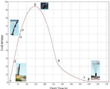
REXUS standard flight profile

The rockets are usually launched under daylight. The rocket accelerates about 26 seconds and reaches a peak acceleration of around 20 g during the boost phase. To be stabilized the rocket goes in to a spin. The spin speed depends on the rocket configuration. The motor burns out around an altitude of 23 km (step 2 in Figure 1.2) and then “glides” the rest of the distance. The engine separation is usually performed before an altitude of 70 km and always before the nosecone separation (step 4 in Figure 1.2). To be stabilized the payload can be separated later. The last separation is on the decent of an altitude of approximately 60 km and is before the vehicle enters the lower atmosphere. On the decent the payload has a maximum

deceleration of 6 g. At an altitude of about 5 km a parachute system decelerates the payload to a velocity of approximately 10 m/s before landing (step 8 in Figure 1.2).

Figure 1.2

(13)

7

1.2 Purpose

Today SSC uses alumina fins with a steel leading edge. The fins are designed by NASA about 40 years ago. With new strong lightweight materials on the market it could be possible to reduce the weight of the fins and thereby reduce the weight of the rocket. With the reduced weight the rocket can reach a higher altitude with less fuel or carry more payload.

The purpose of this thesis is to do a study if it is possible to replace today’s alumina fins with a similar own developed concept composite fin, thus making a big weight reduction and still remaining stiffness and strength.

1.3 Scope of work

 Literature studies about fiber composites properties and processing.

 Estimate the acting loads on the current used fin.

 Optimize the beam structure on the current fin to be able to use the same beam solution in the new developed fin if necessary.

 Make a model of the design concept of the new fin.

 Getting started with FEM.

 Create a decent working mesh of the new fin.

 Start simulating the new fin.

 Interpret and analyze the result of the simulations.

 Improve the composite layup.

 Presentation for SSC Space at ESRANGE and MDH in Västerås.

1.4 Limitations

To make this bachelor thesis within a reasonable size a lot of limitations had to be made. From SSC Space the requirement was that the new fins dimension should be the same as the current fins dimension.

These points have not been covered in this thesis.

 Due to the complexity of aerolasticity it has not been taken into account under the simulations for the current and the new developed fin.

 During the launch the rocket will be exposed to a lot of vibration, and there is no knowledge of the vibrations, nor are the effects of the vibrations known.

 The real attachment area of the fin has not been simulated and considered. The complexity of holes and attachments in composites would require extensive

simulation and analysis in order to correctly capture the behavior. Zero displacement boundary condition for the areas that are in contact with the rocket fuselage has therefore been assumed.

 Possible effects of moisture and manufacturing induced defects.

 The thermal loads that creates internal stresses in the component when processing the component.

 The cost of the material and processing of the new fin has not been considered, but cost saving materials and processing method has been chosen with respect to the costs.

(14)

8

1.5 Supported material

Supported material from SSC Space was a used fin, CAD-geometry for the newer variant of the current fin and flight data and documentation for the REXUS 4 rocket.

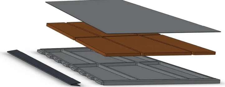
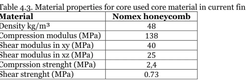
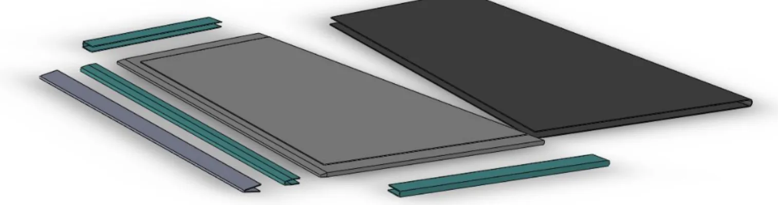
1.6 Description of current fin

The current fin consist of four parts; sheet metal, core material, frame and leading edge. The sheet metal and the frame are made from an aluminum 6061 alloy. The 6061 alloy’s main constituents except aluminum are magnesium and silicon. It is known as a strong alloy which is used widely in the aerospace industry. The fin core consists of Nomex paper in honeycomb structure. The leading edge consists of stainless steel. The sheet metal and the leading edge are fastened to the frame with 2.5 mm screws, and the attachment to the rocket is fastened by 6.8 mm bolts. The core material is adhesively bonded to the frame and the sheet metal. Figure 1.3 illustrates the assembly of current fin.

Figure 1.3 Assembly of current fin.

The current fin has a weight of 5.8 kg. The fins total thickness is 14 mm of which the sheet metal has a thickness of 1.5 mm. The thickness of the leading edge is 1.5 mm. The rest of the fin’s dimensions are illustrated in Figure 1.4.

The current fins are designed to withstand the loadings they are exposed to during one flight. The fins are only used in one flight, after which they are discarded. The fins structure has been optimized over all the operating years. The fins are usually attached to the rocket some days or weeks before flight. The fins position is at the end of the rocket (if it is a single stage rocket). The fins are attached to the rockets tailcan by an aluminum attachment which can be seen in Figure 1.5.

(15)

9 Figure 1.4

Dimensions of the current fin.

Figure 1.5

REXUS rocket with fin attached to tailcan. Figure from Reference [http://www.rexusbexus.net, June 2012].

(16)

10

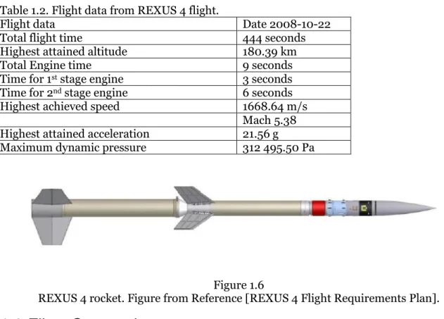
1.7 REXUS 4

The REXUS-4 rocket was launched the 22nd_{September 2008 from ESRANGE in Kiruna. The}

rocket carried five experiments from German and Swedish universities. In Figure 1.6 it can be seen that the rocket was a two stage engine rocket. The first stage was a Nike solid stage and the second stage was an Improved Orion solid stage. Some important data from REXUS 4´s flight are represented in Table 1.2.

Table 1.2. Flight data from REXUS 4 flight.

Flight data Date 2008-10-22

Total flight time 444 seconds

Highest attained altitude 180.39 km

Total Engine time 9 seconds

Time for 1st_{stage engine} _{3 seconds}

Time for 2nd_{stage engine} _{6 seconds}

Highest achieved speed 1668.64 m/s

Mach 5.38 Highest attained acceleration 21.56 g

Maximum dynamic pressure 312 495.50 Pa

Figure 1.6

REXUS 4 rocket. Figure from Reference [REXUS 4 Flight Requirements Plan].

1.8 Fiber Composites

Polymer based fiber composites consist of at least two constituents, resin and fiber. The resins may be either thermoplastic or thermosetting polymers. The fibers usually consist of glass, carbon or aramid. The fibers can be arranged in different configurations in the composite; commonly as plies having straight unidirectional fibers and in various forms of fiber fabrics. The resin is the matrix material that binds the fibers together, that keeps the fibers protected and supports the fibers during compression loading. The matrix material also transfer loads between fibers and fiber layers. The advantage with fiber composites is the high strength to weight ratio. Ordinary construction materials as steel and aluminum have essentially the same material properties in all directions. For fiber composites it is different, a fiber composite is considerably stronger and stiffer in the fiber direction. By placing the fiber layers in selected directions it is possible to control the strength and stiffness. Another difference between composites and metals is that metal components are created from an existing metal by transforming. A composite component is created at the same time the composite is created. This gives possibilities to create components that only can be realized with composites.

(17)

11

1.8.1 Carbon fiber

The carbon fiber is characterized by high E-modulus, high strength, high thermal and electrical conductivity, low thermal expansion coefficient, but has a high cost.

Carbon fibers may be produced from polyacrylonitrile (PAN), carbon and petroleum or synthetic tar precursors. PAN based carbon fibers are produced by wet spinning where the fibers are stretched to give a high grade of orientation of the molecular chains identical like textile fibers. The PAN fibers are then oxidized/stabilized in air with temperatures of 200-260°C before they are carbonized in higher temperatures. Depending on the temperature of the carbonizing stage the material properties changes. In particular cases the fibers are graphitized to get a higher E-modulus, but with the cost of lower strength. These processing stages are illustrated in Figure 1.7.

Figure 1.7

Processing of carbon fiber. Figure from Reference [Damberg, 2001]. Carbon fiber can induce galvanic corrosion in aluminum. To protect the carbon fiber composite/aluminum from corrosion, thin films, surface treatments or layers of glass fiber can be placed at the interface regions. Titanium and steel does not corrode with carbon fiber. Because of carbon fibers high strength and low weight it is widely used in aerospace, military and motorsport industries.

1.8.2 Epoxy

The name epoxy includes several thermosetting polymers. They have in common that under curing it reacts to itself or with a hardener. Typically, epoxies show good mechanical

properties, good temperature resistance, good chemical resistance and good bonding to other materials. Epoxy polymers can normally withstand temperatures of 180°C under shorter times and 130°C under longer times. Advanced epoxy based composites are cured under high pressure and under elevated temperature (usually 120°C-170°C).

(18)

12

1.9 Sandwich construction

Sandwich constructions have been and are today widely used in the aerospace industry. The sandwich construction follows a basic pattern. Two facings which are relatively thin and strong surround a relatively thick lightweight core which can be seen in Figure 1.8. The function of a core material is to stabilize the skin material and carry the shear loads meanwhile the skins or facing take up the bending stresses. By distancing the skins so the moment of inertia is higher, lighter and stiffer constructions may be produced. Also thermal and sound insulating properties, and vibration damping may be improved with this sort of design principle.

Figure 1.8

Sandwich construction. Figure from Reference [Honeycomb Sandwich Design Technology]. Cores can be solids or in other different shapes like honeycomb. The mechanical property of the core is then strongly affected by the core materials mechanical properties. Several properties are also affected by the honeycomb materials geometry. Usually the honeycomb core has different mechanical properties in the W and L direction as seen in Figure 1.9. The cell size impacts the strength between the core and the skin and controls the stress levels when buckling of the cell walls occurs.

Figure 1.9

(19)

13

1.9.1 Core materials

Nomex

Nomex paper is a trademark for aramid fiber paper. It is tough, very light and has high corrosion resistance. It is also very flame resistant and can withstand high temperatures. Due to Nomex cores good mechanical properties it is widely used in interior and exterior parts in the aerospace industry.

Aluminum

Aluminum as a sandwich core has been used in the aerospace industry for a while, but is more and more replaced due to corrosion problems when used with carbon fiber composites. The aluminum can be surfaced to minimize the risk for galvanic corrosion. An alumina core provides a very high strength and stiffness to the construction. 5052-H39 is the most common used alloy.

Rohacell

Rohacell is an expanded plastic core with high strength and thermal capacity. The material can be used up to a temperature of 220°C. The material has good mechanical properties over a wide temperature range. The Rohacell core can be thermoformed into complex geometries.

Divincell HT

Divinycell is a polymer foam material which provides good mechanical properties to a balanced cost. It has high strength to weight ratio. It is very dimensionally stabile, non-hygroscopic and provides good damage performance. Divinycell can withstand temperatures over 100°C and even higher temperatures for shorter periods. It is also used widely in the aerospace industry.

1.10 Processing methods

1.10.1 Prepreg

Prepreg are plies with fiber and resin together, like a fiber tape with impregnated resin. Curing prepregs in an autoclave (pressurized oven) is the most common way to produce high performance composite parts for aerospace applications. The prepreg plies are cut and placed in a mold in the wanted directions. Before the mold enters the autoclave it is vacuum bagged to ensure higher pressures. Because the pressure acts over the whole mold, the mold does not need to be as strong as in ordinary vacuum bagging.

Prepreg is often used when there are high demands on the material due to its good processing quality. The high pressure and temperature under the curing ensures that the material has fewer voids in itself. In the autoclave the material can be exposed to over 7 bars pressure and temperatures up to 250°C. The process is slow, has high costs and is therefore more used for shorter series.

(20)

14

1.10.2 RTM

RTM stands for Resin Transfer Molding and is a closed molding process. It offers

dimensional accuracy and high quality products. The plies are put into to the mold in dry form and then the mold closes. After that the resin and catalyst are injected into to the closed mold and encapsulate the fibers. When the resin has cured the mold can be opened and the finished component removed .The process achieves a fine surface finish. Since the process is closed it is also cleaner and healthier than many other processing methods. In Figure 1.10 the process is illustrated.

Figure 1.10

RTM process. Figure from Reference [http://www.rtmcomposites.com, July 2012].

2. Theory

2.1 Mechanics of composites

2.1.1 Micromechanics

The micromechanics theory can be used to calculate the elastic properties for a single ply. For a single ply a coordinate system can be described by the fibers direction L (longitudinal) or 1. The transverse direction of the fibers in the plane is denoted T- (transverse) or 2-direction as can be seen in Figure 2.1. To describe the in-plane stiffness for an orthotropic composite material four elastic independent constants are needed. For isotropic materials only two independent constants are needed, E-modulus and Poisson´s ratio. The elastic properties of a ply depend directly on the volume of fibers and matrix in the ply.

Figure 2.1

(21)

15

= (2.1) or (2.2) There are different methods to determine the fiber volume fraction of a composite. For glass fiber composites the matrix can be burned off. For carbon fiber composites the matrix is digested by using heated nitric acid so the remaining fibers can be weighted. For a processing method such as RTM the fibers can be weighted before the processing starts. Typical values for fiber volume fractions in commercially composites are 0.4 to 0.7. In a composite the fibers are randomly distributed. However for composites with high volume fraction the fiber tends to be positioned in a more hexagonal pattern. In Table 2.1 it can be seen that hexagonal packing theoretically yields higher fiber volume fraction than square packing.

Table 2.1. Maximum fiber volume fraction of different fiber packing arrangements. Fiber packing method

Square packing 0.79

Hexagonal packing 0.91

Elastic properties

Calculations methods are based on the linear elasticity theory. The non-uniform stress distribution on the micro level has to be averaged to give composite properties on the macro level. The mathematical solutions for elasticity problems may be performed analytically or numerically. Exact solutions are only available for a few cases. Approximate analytical solutions are often based on minimization principles from linear elasticity and numerical methods are usually based on the FEM. The finite element theory usually provides accurate solutions to micromechanics problem.

2.1.2 Calculation models for a composite ply

Rule of mixture

Before calculations can be made the assumptions that fibers are perfectly aligned and there is perfect bonding between the fiber and the matrix are needed. Because the fibers and the matrix are bonded to each other it is a reasonable assumption that the fibers and matrix will deform equally when loaded in fiber direction. The strains in the fiber, matrix and composite as whole are therefore identical.

(2.3)

and thereby is the force P acting on the composite shared by the fiber and matrix

. (2.4)

is the force carried by the fibers and is the force carried by the matrix. The forces are related to the stresses in the load direction by

(22)

16

Where A is the total cross sectional area and the and is the cross sectional area for the fibers and the matrix.

(2.6)

In a unidirectional fiber composite the volume fraction of a component is equal to the components area fraction

and (2.7)

Thereby combining Equation 2.4, 2.5, 2.6 and 2.7 the final form for average longitudinal stress in the composite is

(2.8)

Equation 2.8 is a “rule of mixture” for composite stresses when the loading is in the fibers direction. It is valid for linear and also for non-linear materials.

To estimate the proportion of the stress carried by the fiber the materials properties are assumed to be linear elastic, and by neglecting the Poisson´s effect the stress-strain relationship becomes

, and (2.9)

If the first expression is divided by the second in Equation 2.9 and the limitation from Equation 2.3 is used, a stress ratio between the fiber and matrix is obtained

(2.10) Since the E-modulus for normally used fibers are at least 20 times larger than for the matrix the stress in the fibers is at least 20 times larger than in the matrix. The ratio between the force in the fibers and the matrix is

(2.11)

If Equation 2.9 is substituted into Equation 2.8 the longitudinal E-modulus for a composite can be obtained by the “rule of mixture”

(2.12)

The “rule of mixture” for the E-modulus in the longitudinal direction is a physical reasonable assumption that is very accurate to real composite elastic properties.

The microstructure of a composite exposed to a load in the transverse direction is very inhomogeneous. The local stresses vary in fibers and matrix. To be able to express the stresses mathematically assumptions and simplifications are needed. By replacing ordinary fiber packing with fiber and matrix layers and then replacing that simplification with only two layers, fiber and matrix, the ratio of the thickness of the two layers to the total thickness then correspond to the volume fraction of the fiber and matrix, see Figure 2.6 and

(23)

17 Figure 2.2

Simplification model. Figure from Reference [Varna et al., 1996].

, and where (2.13)

The major Poisson´s ratio of a composite material is defined for uniaxial loading. The first index expresses the direction of the load and the second expresses the direction of the contraction. According to definition Reference [Varna et al., 1996]

(2.14)

Isotropic fibers and matrix is assumed. The Poisson´s ratio for the fiber and the matrix are thereby

and

(2.15)

Applied force in L-direction and equal strain is assumed for the fiber and matrix.

(2.16)

The same assumption of two layers as earlier is also applied (Equation 2.13). The displacement in T-direction for the composite is thereby

(2.17)

The transverse displacements are negative due to related transverse strains

, and (2.18)

If Equation 2.17 and 2.18 is combined and divided by the rule of mixture is formed for the strain in T-direction.

(2.19)

If Equation 2.19 is divided by the rule of mixture for can be written as

(2.20)

The minor Poisson´s ratio can calculated be determined by reciprocal relationship to

(24)

18

Halpin-Tsai

Due to the bad and incorrect results when calculating and with rule of mixture it is better to use the so called Halpin-Tsai method. The Halpin-Tsai equations are semi-empirical functions which are adjusted to fit numerical results in a special range of fiber fraction

volume (45-65 %).

For the transverse E-modulus the expression is

(2.22)

where

⁄

⁄ (2.23)

ξ is a parameter which needs to be determined from a comparison between predictions based on Equation 2.23 and experimental data or results from numerical calculations methods as the finite element method. For fibers with circular cross sections often is used. For smaller fiber volume fractions the method is close to the rule of mixture, but for larger fiber volume fractions the difference becomes significant.

The equation for the in-plane G-modulus is in the same form as the transverse E-modulus equation. (2.24) where ⁄ ⁄ (2.25)

For the G-modulus equation usually is used for circular fiber cross sections.

2.1.3 Elastic behavior of a lamina

Calculations for a lamina which consist of two or more plies which can have different

orientations are a bit different from previous calculations for a single ply. Instead of the fiber diameter as a scale now the ply thickness is the characteristic scale. Since the plies can have different orientations within a laminate, it is necessary to be able to calculate the lamina elastic properties in different coordinate systems. A linear relationship between stresses and strains, negligible out of plane stress components and an idealized geometry (straight parallel fibers with uniform thickness) are assumed.

For a general loading case there are nine stress components characterizing the stress state at a point shown in Figure 2.3. The stress components can be written as a 3x3 matrix and form a second order tensor. Therefore it can be simplified into six independent components.

(25)

19 Figure 2.3

Stresses directions in a composite. Figure from Reference [Varna et al., 1996].

. (2.26)

It is assumed that all out of plane stress components becomes equal to zero.

(2.27)

The same is for the strain components

(2.28)

The remaining stresses can be seen in Figure 2.4.

Figure 2.4

In-plane stresses. Figure from Reference [Varna et al., 1996].

To further understand the calculations for a lamina two general examples of simple load cases are needed.

Load case 1.

A lamina is exposed to a single load in the 1-direction. Due to material symmetry no shear deformations will occur. There will be displacement in all three directions

(2.29)

However, since we only need the in-plane stress-strain relationship the third strain component will be set equal to zero.

(26)

20

The two remaining strains can then be calculated using general structural mechanics

and (2.31)

The same applies for a loading in the T-direction but the strain will be calculated with

and (2.32)

Load case 2.

A lamina is exposed to a single load in the 1,2-plane. Only shear deformation is assumed.

(2.33)

The shear deformations is thereby

(2.34)

From these examples a solution to all deformation problems can be written in matrix-form

{ } [ ]{ } (2.35)

where [ ] is the compliance matrix.

{ } [

] { } (2.36)

where

, , , and (2.37)

If Equation 2.36 is solved with respect to stresses

{ } [

] { } (2.38)

The Q matrix is the stiffness matrix and the inverse to the S matrix.

In reality the loads rarely are in the material longitudinal and transverse directions only. There is a need for one more coordinate system. The first coordinate system will be referred as the x, y-system and the other as the L, T(or 1, 2)-system. The x, y-system is the global system for the whole lamina and the other is the local system for a single ply. This is required to be able to calculate the local stresses and strains in the transverse and longitudinal

directions due to a general loading case. In Figure 2.5 the relation between the L, T-system and the x, y-system is seen.

(27)

21 Figure 2.5

Angle between the global and local system. Figure from Reference [Varna et al., 1996].

Between the global (x) and local (1) systems axis there is an angle Θ which is measured in the counter-clockwise direction, see Figure 2.5. If the stresses are known in the x, y-system the stresses can be calculated in the L, T-system with

{ } [ ] { } (2.39) where [ ] [ ] (2.40) and and (2.41)

The expression for strain transformation is similar

{

} ([ ] ₎ _{

} (2.42)

The stiffness matrix [ ] can be transformed into a global stiffness matrix for the whole lamina by

[ ̅] [ ] _{[ ]([ ]} ₎ _(2.43)

And the same applies for the [ ] matrix by

[ ̅] [ ] [ ][ ] (2.44)

The orientation of the plies in a lamina is usually defined from the top layer to the bottom layer. For example [ ] . That lamina is symmetric around its middle plane and could therefore instead be described as [ ] . It is also balanced because all plies angle has a corresponding negative direction. For example the +45 ply has the -45 ply.

(28)

22

For many reasons it is good to know the stresses and strains in each ply, for example when estimating failure stresses using failure criteria. Using the CLT assumptions, the expression for strain may be described in terms of midplane strains and curvature according to

{ } { } { } (2.45)

where k is the curvature of the laminate.

The stresses in global x, y-direction in each ply with ply index k is given by

{

} [ ̅] {

} (2.46)

Usually the stresses in each ply or for the whole laminate are unknown but forces and force moments applied to the laminate are known. The resultant force component is obtained by integration of the stress distribution through the thickness of the laminate.

{

} ∫ {

} (2.47)

Integration trough the thickness of multiplied with the moment arm with the respect to the middle plane leads to the resultant moment component

{

} ∫ {

} (2.48)

The directions of the forces and moments corresponding to the x and y axis can be seen in Figure 2.6.

Figure 2.6

Force and moments for a composite. Figure from Reference [Varna et al., 1996].

(29)

23 The extensional stiffness matrix [ ] of the laminate

[ ] ∑ [ ̅] (2.49)

Figure 2.7

Illustration of the coupling effects between normal and shear strains. Only possible if and

exists. Figure from Reference [http://de.wikipedia.org/wiki/Klassische_Laminattheorie,

July 2012].

The coupling stiffness matrix [ ] of the laminate [ ] ∑ [ ̅]

(2.50)

For a symmetric laminate matrix [ ] always will be equal to zero.

Figure 2.8

Illustration of coupling stiffness matrix B. Figure from Reference [http://de.wikipedia.org/wiki/Klassische_Laminattheorie, July 2012]. The bending stiffness matrix [ ] of the laminate

[ ] ∑ [ ̅]

(2.51)

Figure 2.9

Illustration of bending stiffness matrix D. Figure from Reference [http://de.wikipedia.org/wiki/Klassische_Laminattheorie, July 2012]. With the new matrices the Equation 2.47 can be rewritten to

{ } [ ]{ } [ ]{ } (2.52)

(30)

24

{ } [ ]{ } [ ]{ } (2.53)

where { } is the midplane strains and { } is the midplane curvature.

2.1.4 Thermal effects on a laminate

It is usually important to consider thermal stresses in laminated composites. Thermal stresses in plies arise when orthotropic fiber materials are used since the thermal expansion coefficient (α) is different in the L and T-direction. The strains due to thermal expansion for a single ply can be described as

{ _{} {} _} _(2.54)

By applying Hooke´s law into the equation thereby the strains can be described in the local coordinate system by

{ } [ ]{ } { _} _(2.55)

and if that equation is solved with respect to the stresses it becomes

{ } [ ]({ } { _}) _(2.56)

If it is a free thermal expansion the stresses becomes equal to zero because { } { _}.

From Reference [Varna et al., 1996] the forces and momentum caused by thermal loads are

{ _{} [ ]{} _{} [ ]{ }} _(2.57)

{ _{} [ ]{} _{} [ ]{ }} _(2.58)

From the Equation 2.58 it can be seen that a symmetric laminate exposed to thermal loads will not be affected by a bending momentum because [ ] for symmetric laminates.

2.1.5 Failure of a laminate

A single ply can fail in several different ways depending on the ply´s properties and external loading conditions. The loading direction with respect to the fiber direction plays a major role.

Longitudinal tension

From earlier assumptions it is known that it is a perfect bonding between the fiber and the matrix, i.e. iso-strain condition is imposed for the fiber and matrix under axial loading. When a ply fails it occurs in a sequence.

First the weakest fiber break and do not carry any more tensile load at the location of the failure. The stress will be redistributed to the remaining fibers in the surrounding region of the damaged site. The next fiber will then break at the same or slightly higher global load. The stress will then be redistributed again. This goes on until it is no whole fibers left. The weakest fiber will fail independently in random locations. Due to the matrix the surrounding fibers around the failed fiber will be exposed to an overload (higher load than their

surrounded fibers). The region of the overload is very small compared to the total specimen size.

(31)

25

Other failures than fiber failures can also occur as matrix cracks, interfacial debond and matrix shear failure which can be seen in Figure 2.10.

Figure 2.10

Failing behaviors for a composite. Figure from Reference [Varna et al., 1996].

Longitudinal compression

When a single ply is exposed to a compressive load the fiber starts to buckle. This can create a shear or extensional failure.

Transverse tension

The transverse tensile strength is dominated by the matrix properties and interface failure. Strong factors of the transverse failure are the fiber volume fraction, the presence of voids and initial defects and fiber debonding.

Transverse compression

A single ply exposed to a transverse compression loading usually fails in shear mode. The matrix deforms plastically and fails in shear because of debonding and fiber crushing.

In-plane shear

The shear strength in the plane is dominated by the matrix and the interfacial properties since cracks spread and can occur when it is pure shear between the fibers.

Stress and strain formulation

As earlier described the stresses can be expressed in three different components. Since failure stress may be different depending on compression or tensile stress there is a need to express the strength in more than three components, as described in Figure 2.11.

Figure 2.11

Stresses in a composite. Figure from Reference [Varna et al., 1996].

(32)

26 Figure 2.12

Strains in a composite. Figure from Reference [Varna et al., 1996].

The sign for each stress direction can be seen in Table 2.2. Table 2.2

Signs for direction.

Number Failure strain

1 + 0 0

2 - 0 0

3 0 + 0

4 0 - 0

5 0 0 ±

Maximum stress criterion

Composite failure will not occur if

(2.59)

(2.60)

| | (2.61)

These criteria can represent a box where the inside of the box represent the stress space that will not make the composite fail. This criterion is easy and simple to use but has its

limitations when there are no interaction effects between the stress components.

When analyzing the failure of a ply it is always done in the local coordinate system since the strength is strongly related to fiber direction.

For example if a single ply is exposed to a uniaxial loading in the x-direction, the local stresses are described as

{

} [ ] { } {

} (2.62)

From Equation 2.41 it is known that and .

Then if the maximum stress criterion is applied, failure in the L-direction is or depending of the direction of the applied load (tensile or compressive).

(33)

27

_, _(2.63)

In the T-direction failure will occur when or .

_, _(2.64)

In shear failure will occur when | | .

(2.65)

If the fiber orientation for the ply ( ) is changed three different modes of failure will appear depending on the fiber orientation as illustrated in Figure 2.13.

Figure 2.13

Relationship between stress at failure and fiber orientation angle. Figure from Reference [Varna et al., 1996].

Maximum strain criterion

Composite failure will not occur if

(2.66)

(2.67)

| | (2.68)

Equation 2.66 to 2.68 can also describe a box as the maximum stress criterion where the strain within the box will not fail the composite. The maximum stress and strain criterion render the same results when the loading is uniaxial, but when the stress state is biaxial the criterions generate different results.

Tsai-Wu criterion

Instead of describing a box where the inside represent the non-failure stress space the Tsai-Wu criterion describes a space given by a second order surface. A second order surface is described by a quadratic equation.

where (2.69)

(34)

28

(2.70)

Equation 2.70 can describe hyperbolic, parabolic and elliptic surfaces but since the surface must be closed only the elliptic surface can be used in a strict sense. To be able to define an ellipsoid the coefficients of the quadratic equation must satisfy some relations.

(2.71)

(2.72)

(2.73)

The coefficients comes from analytic geometry and determine the position of the center of the failure surface, determine the distance from the center to the surface

position and determine inclination with respect to and planes. The calculation of the failure coefficients are based on experimental data.

(2.74) (2.75) (2.76) (2.77) (2.78) √ (2.79)

To be able to calculate the failure for a single ply depending on the fiber orientation requires a modification of Equation 2.70 into

(2.80)

The Tsai-Wu criterion is widely used by simulation programs due to the convenience of having only one equation. It is considered more accurate than maximum stress or strain criterion because it takes stress interaction into account. The only problem is that it is not possible from the criterion to directly determine the failure mode of the failure.

2.4.5 Strength and failure of laminates

The strength of a single ply depends on its orientation against the load direction. For a laminate it is different because of all the plies different orientations. Even for a uniaxial loading all the three stress components are acting at the ply level. For this reason individual plies in a multidirectional laminate will fail at different global strains. The earlier presented failure criteria can only determine a failure for an individual ply. There is no criterion that can calculate the ultimate failure of a laminate. Therefore the failure of a laminate has to be determined by failure of a single or more plies with same orientation in a sequence until all

(35)

29

plies have failed. When a ply has failed it will in reality still carry some load, but to make the calculations simpler in the “ply-discount” model, it is assumed to not carry any more load. For this reason all the carried loads will be transferred to the other remaining plies.

The calculation procedure for failure of a laminate

To determine the failure of laminate the force or moment direction has to be known.

{ } { } (2.81) { } { } (2.82)

where t is the load factor.

1. First must the stiffness matrices ([ ] [ ] and [ ]) for the laminate be calculated. 2. Find the strain of the laminates midplane ({ }) and the curvature of the midplane

({ }) as a function of the load parameter t.

3. Find stresses and strains in local axes of each ply.

4. Use failure criterion for each ply to calculate the load level needed for failure. Find the minimum load that corresponds to the weakest ply failure and note which plies have failed at this load.

5. Have all plies failed? If yes the procedure is complete otherwise assume zero stiffness matrices for failed plies and recalculate the stiffness matrices for the “new” laminate and start at point two again (ply-discount model).

(36)

30

2.5 Finite Element Method

Finite element method (FEM) has become a powerful tool in today’s engineering problems. It can be used in many areas as calculating deformation, stress, heat, flux, fluid flow, magnetic flux, seepage and a lot other flow problems.

2.5.1 History

The basic idea of FEM started from advances in aircraft structures analysis under World War II. In 1941 Alexander Hrenikoff presented a solution to elasticity problems by using a “frame work method” and in 1942 Richard Courant presented a similar solution to model torsion problems. The solutions shared an essential characteristic. They divided continues areas in to smaller discreet sub areas, usually called elements. 1947 Olgierd Zienkiewicz started

gathering those methods together and created what today is called Finite Element Theory. Hrenikoff´s divided his model by using a lattice analogy while Courant used triangulars. In the middle of the 1950´s the development of FEM earnestly began for structural analysis. In the early 1960s engineer used FEM to approximate solutions of stress analysis, heat transfer and fluid flow. The method really started to get handy with the fast computer development of the late 20 century. Today the producer of CAD programs starts to integrate FEM into the CAD programs. That makes the FEM more available to engineers and designers.

A structural problem contains an infinite number of degrees of freedom and is represented mathematically by the multi-variable differential equations. Therefore a structural analysis is described by of multi variable differential equations with boundary conditions. The equations usually have to be solved with numerical methods. By dividing areas and volumes in to elements the degree of freedom is reduced to a finite number. By dividing the model in to elements the model is simplified to better counter the calculation. The characteristic for FEM is the assumption that the elements connection points are connected, usually called nodes. The elements and nodes together represent the mesh. The size of the elements can be varying depending of needed accuracy of that area. By connecting the finite elements with known elastic properties the problem can be transformed to a solution to a linear equation system which describes the force and displacement in the nodes. Depending on the problem and which load and simplifications that have been made to the model different element types are used. Smaller elements in general generate a more accurate solution but of the cost of longer calculation time. Bigger stresses require finer subdivision of elements to generate

convergence of the numerical calculations.

A complete FEM model includes a geometric model, boundary conditions, loads, material models and subdivision elements. The geometric model should be simplified so only the significant details are retained to minimize the number of elements that needs to describe the correct geometry. For structural problems two set of boundary conditions are used, one for displacement and the other for the stress components.

(37)

31

2.5.2 Brief description of the method of static linear structural problems

A structure who is an assembly of a number of elastic elements could be described by the mechanical equation of a spring

(2.83)

i. e. force = spring constant multiplied with the displacement. In this structural problem:

The equation system can be written as ( ) [

] ( ) (2.84)

The unknown displacements can be solved from the equation system by equation ( ) ₍

) (2.85)

and the unknown forces can thereby be calculated by equation

(2.86)

The design of the matrices and the numerical solution method decides the solution accuracy of the simulations. Most of the calculation time goes to calculate the structure stiffness matrix , therefore could many different load cases be calculated with only minor added calculation time. For the calculations of displacement boundary conditions are taken into account. The strain is calculated from the displacement derivatives that are available from the

displacement of the nodes. Within the linear elastic region the stresses can be calculated with Hooke’s law

(2.87)

where is the stress vector with components for normal and shear stresses, the strain vector and the material stiffness matrix.

For plane stress condition and isotropic material:

[ ] (2.88) [ ] [ ] [_] (2.89) ₍ ₎[ ( )] (2.90)

(38)

32

where and are displacements in respective coordinate direction, and strains in respectively direction, the shear angle, the elastic modulus and the Poisson´s ratio. The stresses, strains and displacements are compiled for the whole structure. Values for the nodes are calculated with the displacement conditions for the selected elements.

The displacement conditions describe how the mesh could vary between the nodes. With a known nodal displacement condition in polynomial form the displacement could be calculated at any point in the element. Generally, higher degree of polynomial gives more accurate solutions, but to the cost of longer calculation time.

For a more extensive explanation about FEM the reader is referred to Reference [Persson, 1999] and Reference [Belegundu et al., 2002].

2.5.3 Element types used in Ansys

Solsh190

Solid shell 190 is used for simulating shell structures in Ansys. The shell structures can be thin or thick. Solid shell is a very useful for modeling laminated shells or sandwich

constructions. The element geometry is a six surface cube with eights node, as can be seen in Figure 2.14. There are three degrees of freedom in every node (x, y and z). The element can also be of prism geometry for special occasions where cubes are not desired. The element can be used for a wide range of construction materials.

Figure 2.14

Solsh190 elements. Figure from Reference [Ansys 13.0 Help].

Solid185

Solid 185 is used for solid modeling of solid structures. The element geometry can be a six surface cube with eight nodes, five surfaced prism with six nodes or a four surfaced

tetrahedral with three nodes, as can be seen in Figure 2.15. The tetrahedral geometry is not recommended due to poor simulation quality for this element type. All the nodes for all the different element geometry have three degrees of freedom (x, y and z). The element can be used for a wide range of construction materials.

Figure 2.15

(39)

33

2.6 Flight mechanics

2.6.1 Basic aerodynamic of an airfoil

When an object moves through a fluid the velocity of the fluid will change around the objects surface. Velocity changes of the fluid will create variations of pressure on the objects surface. These pressure variations will create a force that acts on the component. If this object is an airfoil the acting forces will create a lifting force, drag and a momentum. Although an angle of attack is needed to create a lifting force on a flat plate due to its symmetry. When a fluid is passing a curved surface the fluid velocity will increase and the pressure on the surface will drop. Because of the pressure drop it is possible to get a lifting force to act on an airfoil. The acting lifting force will act normal to the airfoils mean camber line. If the lifting force is divided in an x and y component, the y component is pure lift while the x component will generate a backwards acting force. The backward acting force is called drag. There are two types of drag, one is the drag caused by variations of pressure and the other is caused by the friction of the fluid against the surface due to the fluids viscosity. The mean camber line represents the camber of the airfoil by simply going in the middle of the airfoils thickness, as can be seen in Figure 2.16. A symmetric airfoil like a flat plate has no camber. The camber of an airfoil is important if lift needs to be created without any angle of attack. A symmetric airfoil will therefore, not create any lift in no angle of attack.

Figure 2.16

(40)

34

2.6.2 Flat plate in supersonic speed according to shock expansion theory

Consider a flat plate at an angle of attack in a supersonic flow as in Figure 2.17. On the top surface of the flat plate the flow is turned away from itself and thereby an expansion wave occurs at the leading edge. Due to the expansion wave the velocity of the flow will increase and the pressure on the top surface of the flat plate will decrease. At the trailing edge the flow will return to the freestream and thereby a shock wave is created. Because of the shock wave the flows velocity will decrease and the pressure will increase. On the bottom side of the flat plate the flow is returned into itself and a shock wave is created that will increase the pressure but decrease the velocity of the freestream. At the trailing edge the flow is turned into the freestream and thereby creates an expansion wave. The pressure on the top surface is considered as uniform over the whole surface according to the theory.

Figure 2.17

(41)

35

3. Methodology

3.1 CAD-geometry

When meshing and simulating a model, it is important that the model does not have any interactions between parts and, that surfaces and volumes are not too complex shaped. The given CAD-model from SSC Space had to be modified to be able to be simulated, due to interactions between the leading edge, the leading edge attachment on the frame and the skin, see red areas in Figure 3.1. All the modifications were made in a new file were the current fin’s geometry was imported, so no changes to the outer dimension was made. All the parts of the fin were created in one file so that they had geometric relations to each other to ensure a good fit when the fin was assembled. By not merging the different parts in the file it is possible to create the parts in separate files and then later assemble them before meshing and simulating.

Figure 3.1

Red areas illustrate interactions between parts.

The modification on the leading edge was that the side of the leading edge needed to be removed to thereby have the same geometry as the used fin provided by SSC Space. Because the leading edge attachment on the frame did not have the same profile as the leading edge it needed to be modified. Probably there should be a difference of the leading edge and the attachments profile because the leading edge is pressed onto the frame. The modification of the attachment was done so the attachment got the same profile as the leading edge, as can be seen in Figure 3.2. The skin was directly created on the frame to be certain that no

interactions between it and the frame appeared. All holes for screws and bolts were removed to have a simpler simulation model. This also shortened the calculation time.

(42)

36 Figure 3.2

Modulation of leading edge attachment.

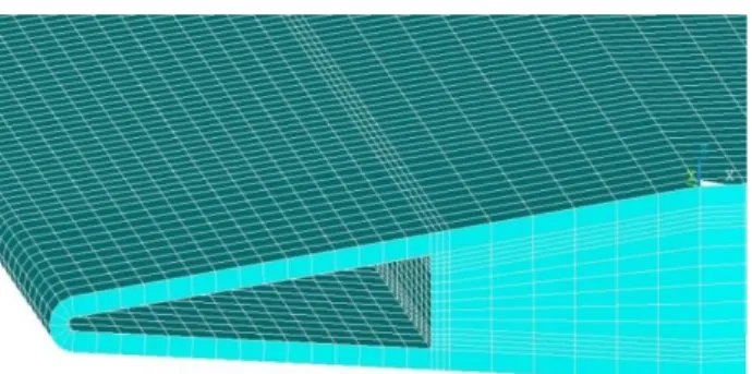
The provided CAD-geometry also lacked core material. The core material was created in the open volumes in the frame, as can be seen in Figure 3.3. The core material is in reality a honeycomb structure, but when modeling core materials with honeycomb structures it should be as solids according to Reference [Honeycomb Sandwich Design Technology]. The mechanical properties provided by the honeycomb structure are therefore specified in the material properties for the core material. Since the core material has different properties in different directions a coordinate system was created for the core. The adhesive between the core, skin and frame was not included in the new model. Due to the low stiffness of the adhesive the structural stiffness of the fin is believed to be unaffected, however, omitting it may affect the strength analysis. Perfect bonding between the parts was assumed in the simulations.

Figure 3.3 Created core material.

All the modifications are relatively small and will probably not affect the simulation results in a negative way. Because the removal of holes the simulated fin will be slightly stronger and stiffer than the original geometry.

(43)

37

3.2 Loads

Before starting simulating the new CAD-geometry the loads acting on the fin had to be considered. From SSC Space flight data and documentation for REXUS 4 was provided to estimate the loads. From SSC Space it was told that the current fin is just able to withstand the loads under a flight. The loads that cannot be determined by the flight data and

documentation may therefore be estimated by testing the maximal loads that the current fin can withstand. To have a safety margin for all the loads under the simulations the calculated loads were enlarged to an even value so the fin probably was exposed to higher loads than the real loads under the REXUS 4 flight.

During launch the rocket will be exposed to heavy accelerations and speeds. From simple aerodynamics the active aerodynamic forces are drag and lift due to the fin working like an ordinary wing. Thermal loads will also be acting on the fin.

The fins purpose are to stabilize the rocket by providing small lifting forces so the momentum around the center of gravity remains zero. Winds and other external disruptions can make the rocket get outside of its flight path. The small lift provided by the fins then makes the rocket return to its flight path.

To estimate how much the lift was, fast calculations of the fin were performed with shock expansion theory. The fin was considered as a flat plate in a supersonic freestream in the calculations. The results contained the pressure difference between the top and bottom of the fin. The pressure difference was put in to the simulation of the current fin in SolidWorks. The results from the simulation of the acting pressures were very excessive. Probably the value for angle of attack was too high. Therefore, it seemed reasonable to see what the amount of pressure the current fin can withstand before the materials start to yield instead. The pressure is considered uniformed on the fins top surface. In reality the pressure of the fin will not be the same all over the fins top surface but it is a fair assumption that is consistent with the shock expansion theory.

The drag could be estimated from the provided flight data for REXUS4 where the dynamic pressure for the whole flight was included. With the dynamic pressure known, the drag could be calculated by a simple aerodynamic “cook book formula” from Reference

[Anderson, 2007].

(3.1)

where q is the dynamic pressure, A the frontal area and the drag coefficient.

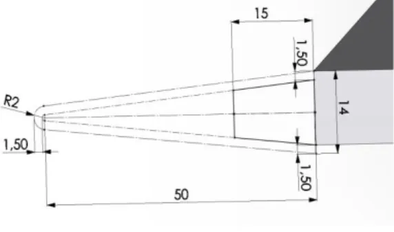
The maximal dynamic pressure was found in tables in the flight data and the frontal area could be estimated from the model in SolidWorks. To estimate the drag coefficient is a rather complicated task and requires a lot of knowledge about aerodynamics. The fin profile can be considered as a flat plate. However since the drag coefficient for a flat plate is equal to zero the calculation will provide zero drag, which is physically unreasonable. Therefore a value for a bullet was found in Reference [http://www.grc.nasa.gov, June 2012]. The assumption may be considered quite rough, but is used to provide an approximate value for the drag. The comparison between the fin and bullets profile can be seen in Figure 3.4.

(44)

38 Figure 3.4 Fin and bullet profile.

The flight acceleration was found in tables in the REXUS 4 flight data. From a table and diagram the maximum acceleration could be estimated. The rocket also does a stabilizing spin under the flight that will provide to accelerate the fin in the spanwise direction (y-direction). This acceleration is so small that it is negligible.

Because the fin reaches such a high altitude the external pressure around the fin will almost be equal to zero and if the fin is airproof an internal pressure will be created under the flight. The thermal loads acting on the fin are very complex to estimate due to the different thermal distribution in the fin. Therefore, thermal effects will not be considered in the simulation. However, it has to be emphasized that the materials used in the new fin design must be able to master the temperatures without failing due to reduced mechanical properties.

The maximal value for these loads has been chosen to be acting at the same time when simulating the fin.

3.3 Simulation of current fin

3.3.1 Preprocessing

Mesh

Before simulating the fin a mesh has to be applied to the model. SolidWorks provides a mesh tool that automatically meshes the model. The fineness of the elements can be decided in a small scale. Due to the poor fineness provided by the automatic mesh tool it was necessary to manually control the size of the elements for particular surfaces. When doing structural simulations it is advisable to use at least four elements in the thickness direction to get a reasonable value for the stiffness of the component. Therefore, small values for the element size were entered. For large surfaces in which edge effects are comparably small there is no need for smaller elements according to Reference [Persson, 1999]. Tetrahedral shaped elements were used because that is the only available element shape in SolidWorks

Simulation. Different size values for the leading edge, frame and skin were used. Figure 3.5 to Figure 3.7 show the refined mesh areas on the current fin.

(45)

39 Figure 3.5

Blue areas represent controlled mesh areas on the leading edge.

Figure 3.6

Blue areas represent controlled mesh areas on the skin.

Figure 3.7

Development of composite fin to Improved Orion rocket.