Modelling the adoption of SPACs with Bass’ diffusion model

School of Education, Culture and Communication Division of

Applied Mathematics

BACHELOR THESIS IN MATHEMATICS / APPLIED MATHEMATICS — MAA322

Modelling the adoption of SPACs with Bass’ diffusion model by

Albin Lindström Jezper Löfberg

Kandidatarbete i matematik / tillämpad matematik MAA322

DIVISION OF APPLIED MATHEMATICS

MÄLARDALEN UNIVERSITY SE-721 23 VÄSTERÅS, SWEDEN

School of Education, Culture and Communication Division of

Applied Mathematics

Bachelor thesis in mathematics / applied mathematics MAA322 Date:

27 May 2021 Project name:

Modelling the adoption of SPACs with Bass’ diffusion model Author(s): Albin Lindström Jezper Löfberg Version: 27 May 2021 Supervisor(s): Fredrik Jansson Reviewer: Thomas Westerbäck Examiner: Doghonay Arjmand Comprising: 15 ECTS credits

Abstract

The recent observed growth in the diffusion of Special Purpose Acquisition Companies phenomena on the U.S stock market may be analyzed from a mathematical standpoint, where

different approaches of the Bass Diffusion Model might be utilized. The Bass diffusion model originates from analysis of product diffusion, where only a few applications have been

seen by financial scholars. The thesis takes a multi analytical approach to examine the phenomena, where multiple regression analysis and Bayesian statistics are used in the parameter estimation processes. Estimated parameter are applied in three different scenarios

of expressing the Bass diffusion model in a discrete time state. By utilizing these different approaches that arise, the study shows that the diffusion of Special Purpose Acquisition Companies Initial Public Offerings in fact can be analyzed from a mathematical standpoint utilizing the Bass diffusion model. Some approaches and scenarios indicate better results in terms of fitting the diffusion, while purposing practical actualities towards the reader and market practitioners. The study further purposes potential modifications that might improve

the results of fitting the phenomena.

Keywords: Bass Diffusion model, Special Purpose Acquisition Companies, Multiple Regression analysis, Bayesian stochastics.

Acknowledgements

First and foremost, we want to thank our supervisor Fredrik Jansson for his invaluable advice, guidance and continuous support during this thesis. We would also like express our gratitude

towards our reviewer Thomas Westerbäck for his important feedback when finalizing the project. Sense this degree is a side project besides our engineering masters, we would finally

like to thank Malin Lundin for her tremendous support and dedication that enabled this opportunity.

Contents

CHAPTER 1

1

1 INTRODUCTION

1

1.1 Purpose 2

1.2 Research Question 3

1.3 Delimitations and validity 3

CHAPTER 2

4

2 FINANCIAL & ECONOMICAL THEORY

4

CHAPTER 3

6

3 MATHEMATICAL BACKGROUND

6

3.1 Bass Diffusion Model 6

3.2 Linear regression analysis 11

3.3 Bayesian Bass Model 14

CHAPTER 4

16

4 METHODS

16

CHAPTER 5

21

5 RESULTS

21

5.2 Bayesian Analysis 26 5.2.1 Presentation of Scenarios based on the Bayesian analysis. 27 5.2.2 Combination of all Bayesian Analysis scenarios 29

5.3 Comparison between analysis methodology 30

CHAPTER 6

32

6 DISCUSSION

32

6.5 Potential modifications and further research 36

CHAPTER 7

42

7 CONCLUSION

42

8 BIBLIOGRAPHY

43

List of Figures

Figure 1: Histrical U.S GDP [9] 5 Figure 2: Historical Proportional Adoption of SPACs in relation to historical IPOs 18 Figure 3: Historical Adoption of SPACs 19 Figure 4: Regression fit of scenario 1a 24 Figure 5: Regression fit of scenario 1b 24 Figure 6: Regression fit of scenario 2a 24 Figure 7: Regression fit of scenario 2b 24 Figure 8: Regression fit of scenario 3a 24 Figure 9: Regression fit of scenario 3b 24 Figure 10: Regression multiplot of all scenarios 25 Figure 11: Trace and density of Bayesian p & q 26 Figure 12: Bayesian fitting with data points, scenario 1 27 Figure 13: Bayesian predicted PDF, scenario 1 27 Figure 14: Bayesian parameter predictions plot, scenario 1 27 Figure 15: Bayesian fitting with data points, scenario 2 28 Figure 16: Bayesian predicted PDF, scenario 2 28 Figure 17: Bayesian parameter predications plot, scenario 2 28 Figure 18: Bayesian fitting with data points, scenario 3 28 Figure 19: Bayesian predicted PDF, scenario 3 28 Figure 20: Bayesian parameter predictions plot, scenario 3 28 Figure 21: Bayesian fitting with data points, all scenarios 29 Figure 22: Bayesian fitting with actual diffusion interval, all scenarios 30 Figure 23: Bayesian PDF predictions, all scenarios 30 Figure 24: Sumuarized plot of scenarios from different approaches. 31 Figure 25: Historical SPAC IPOs and traditional IPOs 32 Figure 26: Manipulate on cumulative adoptation, a(t) and A(t) 37 Figure 27: Manipulate on cumulative proportial adoptation, f(t) and F(t) 37

List of Tables

Table 1: Historical number of SPACs [5] 17 Table 2: Regression coefficients 21 Table 3: Regression parameters 22 Table 4: Residual errors & R-squared regression 23 Table 5: Parameters Bayesian 27 Table 6: Coefficient results, both approaches 31 Table 7: Varaible comaprison with manipulate 37

Chapter 1

1 Introduction

Whenever new products and services are to be launched, projections of future sales may be of interest. What rate of sales should organization expect for a specific product or service? The distribution of sales in a continuous time interval may vary dependent on the situation at hand. One may investigate the possible diffusion of new products or services in a specific market with the Bass diffusion model (BM). The BM are not a new paradigm for studying the diffusion of various goods and services. It has been applied to different cases with various intentions within the mathematical research realm since Frank Bass first introduced the model in 1969 [1]. The various methodologies studied by researchers are based on the basic BM which is one of the most common methods for conducting an aggregated approach. In such approaches, the proportions of people actually adopting the service or product within the total population of potential adopters are modeled [2]. The BM has often been used in applications of modeling diffusion processes due to its simplicity [3]. The mathematical aspects of the BM are highlighted in section 3.1 where three scenarios of expressing the BM in a discrete time state for modelling is expressed. Each alternative way of expressing the BM naturally has its shortcomings but the two latter are considered less appropriate since first has been more applied and entail fewer propagating errors [1,4,5,6,7]. The mathematical level in the study is thought to follow similar simplicity as the BM, with the intention for individuals with less mathematical experience to be able comprehend the methodology as well as the thought outcome.

The BM may in general, be described to incorporate simple factors to which potential adopters are affected to adopt to a phenomenon at hand. Such as through impacts by sorrowing environment or by own free will. The model can be described to only depend on three parameters: innovation, imitation and total population of potential adopters [1]. It is however important to recognize possible limitations that the BM entail, such as the maximum number of potential adopters or that the cumulative adoption by definition is strictly positive [1]. The key elements of the BM are the three parameters. The innovation rate is denoted 𝑝, imitation rate is denoted 𝑞 and potential adopters are denoted 𝑚. Average values of the innovation and imitation rates has through a meta-analysis been determined as 0.03 respectively 0.38 [4]. Various phenomena of diffusion have been studied using the BM, but few researchers have utilized the model in a financial application [1,3,9].

SPAC IPOs (Special Purpose Acquisition Company) (Initial Public Offering) has gained popularity in the last two decades as an alternative to the traditional IPOs process when private companies wish to transform into publicly traded ones. A significant increase in the number of SPACs can be observed in the U.S stock market. In 2020 the number of companies brought to market with SPAC surpassed the traditional IPO process, which may be observed in the historical data of SPAC IPOs presented in Table 1 in section 4.1 [5]. SPAC can simply be described as a method that allows companies to be listed in the stock market in a more time and cost-efficient way compared with a traditional IPO. It is performed by a shell company that

This thesis is intended to investigate the possibility to fit the diffusion of SPAC IPOs with a Bass diffusion model and thus model potential future diffusion of SPAC IPOs. Depending on the potential outcome of the study, the cumulative diffusion shows when SPAC IPOs, in theory, are expected to fully replace traditional IPOs. One may however argue that it is not reasonable to assume that SPACs can be expected to take over the entire market of IPOs, but it does relate to assumptions and restrictions of the BM which ultimately affect the outcome. The model will be fitted utilizing different mathematical methodologies for parameter estimation in the BM. The different methodologies are to be examined and compared to highlight potential differences of the parameter values and projected cumulative diffusion as well as provide the best possible result of modeling the diffusion.

The study thus entails mathematical estimation of the parameters included in the BM, where the programming language R is thought to be utilized. In the light of mathematical adaptation of the BM, two different approaches are applied for estimating parameters based on historical data. Namely, regression analysis together with a Bayesian stochastic approach. These methodologies are to be utilize in order to estimate the parameters and then use three different scenarios of expressing the BM in a discrete time format in order to model the diffusion of SPAC IPOs and compare the possible outcomes. The gathered historical data of the number of SPAC IPOs that has been listed for each year in the time span 2003-2021 in Table 1. It is however important to note in the utilization of data, that there are plenty of factors that affect the number of SPAC IPOs that are listed each year, which is further highlighted in Financial & Economical Theory section 2. Utilizing the Mathematical Background in combination with gathered data, the approximations can be made through a R-scrips which is presented in Appendix A.

The study concludes that scenario 1 may be considered the best alternative to model and fit the diffusion of SPAC IPOs. The concluded outline of the BM should however be looked upon with caution. Scenario 3 could be considered to provide a better fit with the actual data of SPAC diffusion but does contain a possible risk of propagating errors which entail uncertainties. Furthermore, the study concludes that the Bayesian approach outperforms the regression analysis in terms of estimating parameter values which are to be fitted in the BM and compared with actual historical data. Besides this, the study indicates that SPAC IPOs can be projected with the BM. There are although some insecurities affecting the validity of the results which need to be highlighted. These insecurities brought new insights on how the models potential could be modified to cope with the flaws, such that the validity of the approximations might be improved.

1.1 Purpose

The purpose of this study is to investigate the feasibility of applying the Bass diffusion model to the adoption rate and proportional adoption rate of the SPAC IPO phenomena taking place in the U.S stock market. Through an analytical investigation, the various parameters in the BM are to be estimated with historical data via different approaches that are derived and expressed in the Mathematical Background. The results are to be fitted with the BM and compared with historical data. If a close match is achieved, projections can be computed for the future diffusion of SPAC IPOs. The results from the approaches are to be compared such that the purpose of identifying the better methodologies is fulfilled. Furthermore, the study has the purpose of presenting the results of the approximation in practicality, thus providing information for market practitioners that potentially possess less mathematical experience. The investigation will also, to some degree, highlight the possible limitations that relate to fitting

the phenomenon of SPAC IPOs to the BM. Where the study further aims to propose suggestions on how the results could be improved by implementing extensions and modification to the BM such that a higher validity of the results could be obtained.

1.2 Research Question

• How can the Bass diffusion model be utilized to project the future of SPAC IPOs? o What outline of the Bass diffusion model provides the most accurate reflection

of actual SPAC IPOs?

o What does the projected diffusion with estimated parameters of SPAC IPOs entail?

o How can an extension of the Bass diffusion model improve the results of fitting the SPAC IPOs?

1.3 Delimitations and validity

There are several delimitations within the study that should be addressed. First off, it related to what extent the study aims to investigate the pursued phenomenon, SPAC IPOs, from a mathematical standpoint. Where the mathematical contents are rather simple, it relates to intended target reader, of less mathematically skilled individuals as well as the fact that this is a bachelor thesis where the time and resources are limited. It can be argued that better results could have be obtained with a more extensive investigation if more potential estimation approaches would have been examined. Secondly, one may highlight delimitations with the two outlines of BM purposed in this study, regression and Bayesian approach. Both are in a general sense, only considering a minor part of the phenomena such as the number of adopters, imitation and innovation rate together with the total potential population. Which could result in other important aspects not getting considered.

The study might also be delimited by the chosen outline of the basic BM since only the traditional variation is utilized in an absolute manner, this is however addressed in the potential modification discussion in the end of the study. However, if the study would have been more extensive, the proposed and discussed modification could have been further examined and utilized in the outline of estimation. On another note, the study might be delimited by the fact that it only aims to investigate the current and future diffusion of SPAC IPOs which can be comprehended as only a small part of understanding the phenomena. These delimitations and how to cope with them in relation to the results will further be discussed in section 6 at the end of this study.

From a validity perspective, this study might portray some complications. Such as the utilized literature for the theoretical background and the digital and non-peer-reviewed sources that occur in some cases throughout this study. While the information and knowledge of these sources are founded and build on peer-reviewed material, the content by itself is not. These instances are however represented mainly of mathematical proofs and data collection, which might induce some validity sense mathematics can be portrayed as viable if the mathematics behind them adds up. One may however note that in most cases at which such questionable sources occur these are supported, to some extent, with peer-reviewed articles.

Chapter 2

2 Financial & Economical Theory

SPACs can be described as empty shell companies that are published on the stock market. It is corporations without any operations or business plans that exist with the intention of merging or accumulating a non-published operating company in order to publicize them without going through a traditional IPO process [6]. It is an alternative way for companies to get published on the stock market, with a faster and cheaper process in comparison with a traditional IPO [7]. The SPAC process might, however, bring some drawbacks. Drawback in terms of the fact that the shareholders must agree and support the acquisition, which might give rise to confusion in the merger, that is set out to be performed. At the same time, they do not need to convince a group of investors, as had to be a necessity in a traditional IPO process. Furthermore, current owners of private companies may be concerned about a takeover due to the use of the warrants owned by SPAC backers, dilution of their holdings when using a SPAC acquisition [7]. In the U.S stock market the first SPAC to go public was introduced and publicized in 2003. It was the only published shell company in that year, and it raised $24 Million in capital. The market for SPACs grew rapidly until 2007, where in that year, 66 SPACs where introduced, amounting to $12.1 Billion in raised capital. At the peak of that decade, SPACs represented one third on the total number of companies that went public in the U.S markets. In 2008 as with many investment forms, the SPAC diffusion saw a downturn due to the financial crisis. As a consequence, the diffusion process basically restarted with only 25 introduced SPACs the years of 2008, 2009 and 2010 [8]. One may highlight a correlation between the published number of SPAC and market status. In order to assist a correlation, a description of the market status is important. Traditionally, a bull market is times in which the economy is good, and individuals and companies are willing to invest, this can be considered the case when the number of SPAC IPOs are increasing. On the other hand, a poor economy is referred to as a bear market at which individuals and companies are much more cautious [7]. One may simply relate the historical state of the economy in the U.S to the gross domestic product (GDP) which is presented in Figure 1. When the GDP stagnated in 2007-2009, a poor market status can be identified, a bear market which relate to the decrease in SPAC IPOs in these years. One may, besides recent years positive GDP and bull market, also relate recent increase in the number of SPAC IPOs to the large coverage in media and that it has become a global trend in terms of financial investment.

Figure 1: Histrical U.S GDP [9]

After the financial crisis, with a recovering market status, the number of SPACs introduced on the U.S stock market has risen continuously. Where the year 2020 can be portrayed as the largest shift yet, with 248 SPACs published [10]. This growth has increasingly continued into the current year of writing this thesis (2021), where 308 have been published to date [5]. One reason for the increase of SPAC IPOs is that there exists a significant upside for the creators or founder of these SPACs, undependably if a merger take place or not together with a grater media coverage [11]. Still, the capital surrounding SPAC IPOs can be considered significant since it is corporations with no operations. One may examine Table 1 in section 4.1 which illuminate the gross proceeds of SPAC IPOs each year as well as the gross proceeds of traditional IPOs for comparison. One may note that in 2020 SPAC IPOs represented 55% of the entire number of IPOs on the U.S market. The 248 published SPAC IPOs collectively had gross proceeds of $83 Billion compared with all IPOs which collectively had $179 Billion; thus, the gross proceeds of SPAC IPOs are less than 55% which indicate some cost efficiency. There is however a risk embedded with SPAC IPOs since it solely is a shell corporation at first. It is further noteworthy that not all published SPACs perform mergers with operating corporations, since a merger by regulations, has to be complete within two years of entering the U.S stock market [11]. With the basic assumptions that follow the BM, which are further addressed in the following section, such market failure is not accounted for. The diffusion is solely referred to as SPAC IPOs regardless of an achieved merger or not.

1,00E+13 1,10E+13 1,20E+13 1,30E+13 1,40E+13 1,50E+13 1,60E+13 1,70E+13 1,80E+13 1,90E+13 2,00E+13 2,10E+13 2,20E+13 2,30E+13 2003 2004 2005 2006 2007 2008 2009 2010 2011 2012 2013 2014 2015 2016 2017 2018 2019 USA GDP

Chapter 3

3 Mathematical Background

3.1 Bass Diffusion Model

The BM is commonly applied for modeling and forecasting processes within the research field of marketing but has also been used in other disciplines [3]. The forecasts that the model produce may vary in appearance, but the most common and generally recognized in various research fields is the typical S-shaped curve which displays the cumulative adoption of a phenomenon. The BM forecasts how adoption of a studied phenomenon in some markets may turn out to be at time t if one considers the fundamental aspects of how potential adopters may be influenced [1,3].

In simple terms, the basic BM is utilized to describe the adoption rate over a continues time interval where two or three parameters are included dependent on how one wish to present the diffusion process and the format of historical data [1]. The parameters within the BM are 𝑝, 𝑞 and 𝑚 which constitute i.e., Theorem 2 [1,2,3,17]. The first parameter, 𝑝, are the innovation rate which can be interpreted as to what extent the potential adopters embrace the phenomena by their own innovative self without any influence by others. The second parameter, 𝑞, are the imitation rate which may be described as to what extent potential adopters are affected by others to adopt to the phenomena. The last parameter, 𝑚, are the maximum number of potential adopters that may embrace the phenomena [3]. Hence, the level of maturity that can be expressed for the phenomenon [1,3]. One may however note that 𝑚 may or may not be included in the outline of the BM dependent on the situation at hand which is further addressed in connection to equations (2) and (3).

The rate of diffusion in the BM can be described as a likelihood function and does therefore, similar to likelihood functions in general, depend on a probability density function (PDF), 𝑓(𝑡), in order to distribute the adoption rate over a time interval [1]. The primitive function of the PDF is described by the cumulative distribution function (CDF), 𝐹(𝑡). The relation of these may, by definition, be described by:

𝐹(𝑡) = + 𝑓(𝑡)𝑑𝑡,! " 𝐹(0) = 0, where 0 < 𝐹(𝑡) < 1, 0 < 𝑓(𝑡) < 1. (1)

Simply put, one can view the CDF as the percentual proportion of the total potential population that has adopted to the phenomenon at hand and should thus increase at all times. One may also note that the CDF and PDF are the functions of interest in terms of visualizing the BM, and thus providing potential projections over a set time interval of 𝑡, where the CDF may be visualized as the typical the S-shaped curve [1]. The derivation of the BM relates to the expression on Definition 1 which satisfies the Hazard rate at the left-hand side, since the time to adoption are considered a random variable with the CDF and the PDF. For clarification, the

left-hand side may be read as the proportion of potential adopters who adopts at time t, given that they have not adopted earlier. The right-hand side on the other hand is a linear function with the intercept equal to the innovation rate, 𝑝, and the slope as the imitation rate, 𝑞, multiplied with the cumulative number of adopters [3]. The linear function provides an expression for the extent at which potential adopters are affected, thus if the cumulative number are larger then, potential adopters are more likely to adopt since the product becomes larger. It is further important to highlight the limitations and assumptions within the BM. For instance, that there assumed intervals for parameters, which are stated below, and that there is a maximum number of potential adopters in the population, 𝑚. Another important aspect to take into consideration when applying the BM is that adopters are only permitted to do one adaptation and cannot undo the adaptation which follows the definition of CDF.

Definition 1

#(%)

'()(%)= 𝑝 + 𝑞𝐹(𝑡), 𝐹(0) = 0, 𝑤ℎ𝑒𝑟𝑒 𝑝 > 0,

𝑞 > 0 .

Furthermore, the total number of adopters at time t can be expressed as 𝐴̅(𝑡) and may be considered a random variable in a continues time state dependent on the CDF and the total number potential adopters, 𝑚, equation (2). Thus, if one would like to include the total number of potential adopters, 𝑚, within the BM, one may utilize the expression for the expected average cumulative number of adopters below [3]. With respect to the potential population at hand, an expression for the likelihood function follows as well, by definition:

𝐴̅(𝑡) = 𝐸(𝐴(𝑡)) = 𝑚𝐹(𝑡), (2)

*+̅(%)

*% = 𝑎@(𝑡).

(3)

If one where to adopt the BM to a potential population, and not express the diffusion as a percentage of a fictive population as the case when solely utilizing CDF, as expressed in Definition 1. The two equations above, (2) and (3), should be substituted in Definition 1 similar to equation (5). It does however often depend on the data at hand if one chooses to study the diffusion trough 𝐹(𝑡) or 𝐴̅(𝑡). Two different theorems are presented below which review the different options to study the diffusion with BM. The theorems follow from Definition 1 where the expressions are rewritten with simple algebra and expressed as the PDF, 𝑓(𝑡), or the adoption rate, 𝑎(𝑡) respectively. The 𝑃𝑟𝑜𝑜𝑓 of Theorem 1 is rather straightforward with simple algebra. The 𝑃𝑟𝑜𝑜𝑓 of Theorem 2 does on the other hand include Equation (2) and (3) to illustrate the substitution and thus rather depend on the cumulative adoption as the response variable and does not include a percental relation to the total adoption but rather a finite value, 𝑚.

Theorem 1 _{𝑓(𝑡) = 𝑝 + (𝑞 − 𝑝)𝐹(𝑡) − 𝑞𝐹(𝑡)-.} Proof c #(%) '()(%)= 𝑝 + 𝑞𝐹(𝑡) ⟺ 𝑓(𝑡) = F𝑝 + 𝑞𝐹(𝑡)GF1 − 𝐹(𝑡)G ⟺ 𝑓(𝑡) = 𝑝 − 𝑝𝐹(𝑡) + 𝑞𝐹(𝑡) − q𝐹(𝑡)- _⟺ 𝑓(𝑡) = 𝑝 + (𝑞 − 𝑝)𝐹(𝑡) − q𝐹(𝑡)- ₍₄₎ Theorem 2 _{𝑎@(𝑡) = 𝑝𝑚 + (𝑝 − 𝑞)𝐴̅(𝑡) −} . /𝐴̅(𝑡)-. Proof By Equation (2): 𝐴̅(𝑡) = 𝑚𝐹(𝑡) ⟺ 𝐹(𝑡) = +̅(%) / By Equation (3): 𝑎@(𝑡) = m𝑓(𝑡) ⟺ 𝑓(𝑡) =01(%)_/ ⟹ By Definition 1: _'()(%)#(%) = 𝑝 + 𝑞𝐹(𝑡) ⟺ 𝑎@(𝑡) 𝑚 1 −𝐴̅(𝑡)_𝑚 = 𝑝 + 𝑞𝐴̅(𝑡) 𝑚 ⟺ 𝑎@(𝑡) 𝑚 − 𝐴̅(𝑡)= 𝑝 + 𝑞 𝐴̅(𝑡) 𝑚 ⟺ 𝑎@(𝑡) = 𝑝F𝑚 − 𝐴̅(𝑡)G + 𝑞 𝑚𝐴̅(𝑡)F𝑚 − 𝐴̅(𝑡)G ⟺ 𝑎"(𝑡) = 𝑝𝑚 + (𝑝 − 𝑞)𝐴̅(𝑡) − 𝑞 𝑚𝐴̅(𝑡)!⟺ 𝑎@(𝑡) = 𝑝(𝑚 + 𝐴̅(𝑡)) − 𝑞𝐴̅(𝑡)(1 + 𝐴̅(𝑡) 𝑚 ) (5) (6)

One can recognize that Theorem 1 and Theorem 2 are fairly similar differential equations with similar proofs. The difference is however quite clear, the first does not include the total potential population, 𝑚, and has CDF as response variables. The latter includes 𝑚 due to the expected average cumulative number of adopters 𝐴̅(𝑡) which is the response variable in this case [1]. The differential equations may be solved and thus only depend on the parameters included in the BM as well as time 𝑡. The choice of theorem that is to be utilized depends on the situation at hand and primarily on the format of the data. If you for instance have data of a phenomenon presented as a proportion of all similar phenomena, you would choose the first theorem rather than the second. The solutions to the differential equation in Theorem 2 are expressed in Equation (7) and (8), one may however note that the solutions to Theorem 1 also may be observed if 𝑚 are canceled [3].

𝐴̅(𝑡) = 𝑚𝐹(𝑡) = 𝑚 K'(2"($%&)( '3&_$2"($%&)(L,

(7)

𝑎@(𝑡) = 𝑚𝑓(𝑡) = 𝑚 M4(43.)_(43.2"($%&)()2"($%&)(₎₎N. (8)

To execute the mathematical modeling and forecasting of certain phenomenon, i.e., SPAC IPOs, the parameters in the expressions above need to be determined. The visualization of the equations (7) and (8) are the result of the projection over some continuous time interval T. There exist numerous different procedures for estimating the included parameters of the standard BM [12]. We will investigate the possibilities and differences between linear regression and with Bayesian statistics as estimation methods. It is two very different approaches for implementation of the BM and there exist several other potential methods as well that are not considered [13].

For such approximation methods to be utilized, the model needs to be expressed with discrete time observations with constant data-collection time intervals, rather than continuous. It is crucial in order to avoid circular and inconsistent relationships that may occur when data is utilized in the model to estimate the parameters [3,5]. It is however worth noting that Theorem 1 and Theorem 2 are expressed as dependent on F(𝑡)and 𝐴̅(𝑡), respectively, which may be viewed as values for specific points in time, rather than any non-negative value of continuous time which defines t [14]. The theorems are however still not expressed in discrete time, hence 𝐴₅ = 𝐴(𝑡₅), 𝑖 = 0,1, . . . , 𝑇, where each point in time has a corresponding incremental number of adopters [3]. One may again highlight the importance of the solutions to the differential expressions of the theorems and the interplay that by definition exists between CDF and PDF. One may further express the BM in a discrete time state dependent on the situation at hand and personal preferences as long as the relation between the CDF, PDF and included parameters remain.

One could simply conclude different ways that one intuitively can rewrite the solutions of the differential equation, (7) and (8), in Theorem 1. First it is important to highlight that the two solutions are consistent with each other since they are based on the same differential equation.

(1). Since the cumulative adoption at time 𝑡 is of interest rather than the adoption rate at time 𝑡 one may express the computation of the cumulative adoption approximation in a discrete time domain with three scenarios, where each scenario may be express based on Theorem 1 or Theorem 2 dependent on the dataset, the a and b part of the scenarios, respectively [3,4,5]. In the first scenario, the CDF is expressed similar to continuous time state of equation (7). The difference in the scenario is the PDF which is expressed as the subtraction between the cumulative distribution at time 𝑡 and time [𝑡 − 1], hence the average rate of adoption over the interval [t − 1, t]. It may be considered an advantage for the scenario due to further numerical accuracy since the subtraction are made with two similarly scaled numbers. The scenario may be considered appropriate when approximation of parameters is to be made with for instance Non-linear Least Square (NLS). Historically one may note that this scenario often has been utilized in different diffusion processes due to the interest of the CDF [4,5,6,7]. As follows:

Scenario 1 a. 𝐹(𝑡) =_'3'(2&"($%&)( $2"($%&)( . b. 𝐴̅(𝑡) = 𝑚 U_'3'(2&"($%&)( $2"($%&)( V. (9) a. 𝑓(𝑡) = W_{𝐹(𝑡) − 𝐹(𝑡 − 1), 𝑡 > 1} 𝐹(𝑡), 𝑡 = 1X. b. 𝑎@(𝑡) = W𝐴̅(𝑡), 𝑡 = 1 𝐴̅(𝑡) − 𝐴̅(𝑡 − 1), 𝑡 > 1 X. (10)

The second scenario may be considered to be the other way around, where Equation (8) for determining the PDF remains and the CDF are determined by summarizing all previous rates up until and including time 𝑡. It is however worth to note that the second scenarios may be considered less appropriate since 𝑓(𝑡) expresses the rate at a specific time within the interval [𝑡 − 1, 𝑡] rather than the average rate for the interval as expressed in Equation (10). Hence, 𝑓(𝑡) may be higher or lower than the average depending on the parameters and may thus affect the outcome of approximation as well as future projections [14]. The equations for the second scenario do however follow:

Scenario 2 a. 𝐹(𝑡) = ∑% 𝑓(𝑖) 56" . b. 𝐴̅(𝑡) = ∑% 𝑎@(𝑖) 56" . (11) a. 𝑓(𝑡) =4(43.)_(43.2"($%&)()2"($%&)(₎₎. b. 𝑎@(𝑡) = 𝑚 Z4(43.)_(43.2"($%&)()2"($%&)(₎₎[. (12)

The third and last scenario that may be expressed in terms of rewriting the differential equation of theorems straight away into a discrete time-domain and does not utilize the solutions of the differential equation. The CDF at time t is however expressed as the sum of CDF at time 𝑡 − 1 and PDF at time 𝑡, thus the rate of change in the interval [𝑡 − 1, 𝑡] is added to the cumulative

adoption. One may however note that usage of the third scenario may be considered to conduce errors in the determination and projections of CDF as well as PDF. Unnecessarily large errors may be considered to occur due to the fact that 𝑓(𝑡) is a function of 𝐹(𝑡) which in turn is a function of 𝐹(𝑡 − 1) and 𝑓(𝑡). Thus, if an error occurs in the determination of 𝑓(𝑡) at time 𝑡, the error will propagate and appear larger at time 𝑡 + 2 which in turn results in an unreliable model. A relation can also be made to the parameters within PDF that are to be approximated, 𝑝 and 𝑞, since larger values for these result in a larger 𝑓(𝑡) and thus a larger error [14]. The expression for scenario three follows below:

Scenario 3

a. 𝐹(𝑡) = F(t − 1) + 𝑓(𝑡).

b. 𝐴̅(𝑡) = 𝐴̅(t − 1) + 𝑎@(𝑡). (13) a. 𝑓(𝑡) = 𝑝 + (𝑞 − 𝑝)𝐹(𝑡 − 1) − 𝑞𝐹(𝑡 − 1)-_.

b. 𝑎@(𝑡) = 𝑝𝑚 + (𝑝 − 𝑞)𝐴̅(𝑡) −_/.𝐴̅(𝑡)-_. (14)

The different scenarios to rewrite the BM into a discrete time-domain may thus be applicable in fitting of estimated parameters. The parameters in the BM, 𝑝 and 𝑞 (as well as 𝑚 depending on the theorem that are chosen for further investigation), does however need to be estimated before the scenarios are applied in plotting the diffusion of SPAC IPOs.

3.2 Linear regression analysis

The scenarios above are studied to illustrate their differences as well as the applicability to model the diffusion of a phenomenon, SPAC IPOs, with the BM. In order to examine the applicability of the BM, estimation of parameters is required. A rather simple way to perform a parameter estimation is through multiple linear regression where the characteristic values, β_", β_' and β_-, are to be estimated and then substituted to compute the correct parameters. The theorems may thus by applied in the regression analysis due to the similarities with the general expression for multiple linear regression [15], illustrated below. One may however notice the taper to regression with Theorem 2 of regression analysis due to the available data at hand where the number of historical SPAC IPOs each year may be described as the adoption rate. On may also clarify the relation between the regression coefficients and the parameters in the BM, which the regression is based on, below. The, 𝑦₅, regressors in the regression analysis described below are thus equal to the rate of adoption, 𝑎@(𝑡), and the response variable, 𝑥₅, is the Proportional adoption, 𝐴̅(𝑡), which ultimately describe the diffusion of SPAC IPOs [1,7].

By the general equation for multiple linear regression y₈ = β_"+ β_'x₅+ β_-x₅- _{+ ε,}

one can use

Theorem 2, a@(t) = pm + (p − q)Af(t) −_:9Af(t)-_, Where the characteristic values follow due to similarities:

y₈ = a@(t), 𝑥₈ = 𝐴̅(t), β" = 𝑝𝑚, β_' = 𝑞 − 𝑝, β- = − 𝑞 𝑚.

In order to estimate the characteristic values of multiple linear regression one may use NLS estimation which simply may be described as the minimized squared distance between the actual and estimated regressors [1]. NLS estimation can be described as one of the simpler methods to estimate values in a regression analysis. It does however have shortcomings that are worth to remember in the estimation process. The first is the risk of unstable estimates which possess the wrong signs when a dataset with few datapoints is utilized. The second relate to the right-hand side of Theorem 2 in the estimation which may tend to overestimate the derivative of 𝐴(𝑡) for time intervals before the point of the inflection and underestimate afterwards [16]. When the characteristic values have been estimated trough NLS, the next step is to fit the given regression coefficient to the theorem of the utilized case based on the similarities above [16]. Hence:

𝛽" = 𝑝𝑚 ⟺ 𝑝 = 𝛽_" 𝑚, 𝛽- = − 𝑞 𝑚⟺ 𝑞 = −𝛽-𝑚.

By substitution 𝛽_' can be expressed as: 𝛽' = 𝑞 − 𝑝 = −𝛽-𝑚 −

𝛽_" 𝑚.

The expression can be formulated dependent on 𝑚 as:

𝛽_-𝑚-_{+ 𝛽}

'𝑚 + 𝛽" = 0.

The solution to the second order differential equation are:

𝑚 = 𝑚𝑎 𝑥 ⎝ ⎛−𝛽'± k𝛽' -_{− 4𝛽} "𝛽 -2𝛽 -⎠ ⎞.

It may be expressed as:

𝑝 =𝛽'− k𝛽' -_{− 4𝛽} "𝛽 -2 , 𝑞 =𝛽'+ k𝛽' -_{− 4𝛽} "𝛽 -2 . (15) (16) (17)

In an estimation process, the accuracy of estimated characteristic values is of interest and may be studied trough the 𝑅-_{-value of the estimation. The value of 𝑅}- _{and the relation that it has to} NLS estimation relates to the total error which are divided into two separate parts. The first error originates from the regression and are expressed as the squared distance between estimated response and the average response value. The second error originates from the residual error and are expressed as squared distance between the true response and estimated response value [15]. Thus, in relation to the origin of the errors and equation (20) which may be utilized to compute 𝑅-_{, a larger 𝑅}-_{-value imply a higher degree of explanation in the} executed estimation model. One may also note that if the 𝑅-_{-value are in the interval between} 0.7 and 1 but approaches 0. 7 it can be portrayed as the fit of estimation model becomes more imperfect [17]. The 𝑅-_{-value may thus be expressed as the ratio between the regression error} and the total error term as follows:

𝑆𝑆_!;%0< = 1 𝑛sFf(𝑡) − 𝑓̅(t) G -= %6' ⟹ 1 𝑛sF𝑓u(𝑡) − 𝑓̅(𝑡)G -= %6' +1 𝑛sFf(𝑡) − 𝑓u(𝑡)G -= %6' = 𝑆𝑆_>?@+ 𝑆𝑆_>?A (18) (19) 𝑅- ₌ AA*+, AA-.(/0= 1 − AA*+1 AA-.(/0. (20)

The 𝑅-_{-value does primarily provide an indication of how well fitted the chosen regression} model are. Additional statistical measures may be highlighted to further provide insight in if the parameter estimation can be considered accurate or not. The traditional t-value are utilized in the results to highlight the stability of the estimation, where a value close to 0 are considered more accurate than a value far from 0. The t-value may further be utilized to compute a p-value which provide a likelihood scenario in which we can choose to reject the null hypothesis that all regression coefficients are 0 or not. Thus, with higher probability, higher p-value, the likelihood that the regression coefficients are 0 is larger and we can thus not reject the null-hypothesis. Preferably the p-value is small so that at least one estimation coefficient is separated from 0.

3.3 Bayesian Bass Model

A more complex alternative to estimation the parameters within the BM through a Bayesian statistics and a Bayesian analysis. The fundamental understanding behind the Bayesian approach is presented together with a hypothetical example in order to clarify the different aspects that it may entail. WithinBayesian statistics, probabilities are often used to measure uncertainties in the interface [18]. In the case of this study, uncertainties relate to the future diffusion of SPAC IPOs and the possible effect by the U.S stock market. For the probability distribution can be expressed as follows:

𝑑𝑖𝑓𝑓𝑒𝑟𝑒𝑛𝑐𝑒 ~ 𝒩(𝜇, 𝜎-_). (21)

The distribution above is further used in quantifying the parameters in the BM in a sense of Bayesian statistics. When new data and information is gathered, the previous data are updated, resulting in posterior perceptions. Statistical inference reduces the need to apply probability rules since parameters are given an individual distribution [18]. Furthermore, a Bayesian approach provide a comprehensive and powerful way of modelling estimations and forecasting. When sampling data with Bayesian creates a full distribution profile with parameters, such as median, means and percentiles. The Bayesian approach also has advantages over classical statistical estimation approaches, by using evidence from historical data together with cumulative data. In relation to classical estimators the Bayesian approach is said to be an improvement. This because of the prior knowledge applied and the ability to introduce new or extra data together with the likelihood, result in the posterior estimates being more precise [19].

𝑃𝑜𝑠𝑡𝑒𝑟𝑖𝑜𝑟 = 𝑝𝑟𝑖𝑜𝑟 × 𝑙𝑖𝑘𝑒𝑙𝑖ℎ𝑜𝑜𝑑 𝑚𝑎𝑟𝑔𝑖𝑛𝑎𝑙 𝑙𝑖𝑘𝑒𝑙𝑖ℎ𝑜𝑜𝑑

Analysis based on Bayesian statistics offers a different approach then other classical alternative. In the sense of classical analysis, 𝜃 is usually denoted as the parameter for an unknown constant that represents the current data used to estimate the true value and in terms of probability in the data space. Even though this is the methodologies usually applied in classical inference, it can be said that the Bayesian frameworks suits these interpretations in a more natural way. Since Bayesian inference involves the learning process of changing the initial probability statements regarding the priors of the included parameter together with the ability to update with posterior knowledge and incorporating the given data and prior knowledge [19].

To exemplify this, we denote 𝑃(𝜃) as the prior belief, which in relation to the phenomenon of SPAC IPOs refers to the historical diffusion. Due the prior beliefs for 𝜃, the probability for the data represented by the variable 𝑦 has its conditional probability expressed as 𝑃(𝑦|𝜃). In line with Bayes theorem this updated conditional probability for 𝜃 can be expressed as:

Definition 2 _{𝑃(𝜃|𝑦) =} 𝑃(𝜃) × 𝑃(𝑦|𝜃)

𝑃(𝑦) .

Where 𝑃(𝑦) can be portrayed as the probability for the average data. As presented in equation (21), this can also be described as the marginal likelihood. In this example 𝑃(𝑦) is the total likelihood. From Definition 2 with the rule of joint probability for both 𝑦 and 𝜃 we get:

𝑃(𝑦, 𝜃) = 𝑃(𝑦|𝜃) 𝑃(𝜃) = 𝑃(𝜃|𝑦) 𝑃(𝑦). (22) Where 𝑃(𝜃|𝑦) denotes the probability for the posterior or updated probability beliefs in regard the previous data. It can be described as it takes the priors data with evidence at hand. It is also important to note that 𝜃 can represent hypothesizes, models and/or parameters. Because we portray 𝜃 as this and that it is of random character together with the divisor 𝑃(𝑦) in Definition 2 that is dependent of 𝜃 it can be re-expressed as:

𝑃(𝜃|𝑦) ∝ 𝑃(𝑦|𝜃) 𝑃(𝜃). (23)

Where ∝ signifies expected equality for a proportional constant [19]. This may be explained in words as:

𝑃𝑜𝑠𝑡𝑒𝑟𝑖𝑜𝑟 𝑑𝑖𝑠𝑡𝑟𝑜𝑏𝑢𝑡𝑖𝑜𝑛 =𝑙𝑖𝑘𝑒𝑙𝑖ℎ𝑜𝑜𝑑 × 𝑝𝑟𝑖𝑜𝑟 𝑑𝑖𝑠𝑡𝑟𝑜𝑏𝑢𝑡𝑖𝑜𝑛_{∑(𝑙𝑖𝑘𝑒𝑙𝑖ℎ𝑜𝑜𝑑 × 𝑝𝑟𝑖𝑜𝑟)} . (24)

Where ∑(𝑙𝑖𝑘𝑒𝑙𝑖ℎ𝑜𝑜𝑑 × 𝑝𝑟𝑖𝑜𝑟) is a fixed and normalized factor that makes sure that the probabilities for the posteriors sums to one, hence:

Chapter 4

4 Methods

4.1 Data

The data used in the models for the study is made up of number of the historical SPAC IPOs that has been introduced in the U.S stock market each year. It is worth to note that the data include all IPOs in the U.S, hence all of the various stock exchanges that exists. The data include the number of SPAC IPOs issued in each year from 2003 to 2021, as well as the total number of IPOs performed each year. The data also provide an insight of the total gross proceeds for each year. The data is available at spacdata.com, which is operated by SPAC Analytics, the largest provider of SPAC data and analysis to portfolio managers in the United States [5]. The most recent year, 2021 is as of the first quarter due to the point in time at which data is gathered. Hence, not the complete statistics for the whole year. Quarterly data for previous years is however not available.

In the 18-year time period presented in Table 1, the total number of SPAC IPOs that has been performed sums to 920 instances. Figure 3 shows an illustrative image of how the number of SPACs has varied through the years. In terms of the data at hand, you may note that the diffusion of SPACs has not always been increasing. It is however most likely related to the different factors of the world economy, and primarily the US economy which is highlighted in section 2: Financial & Economical Theory . Figure 1 shows the GDP of the US where one can highlight the dip as a result of the financial crisis 2007/2008 which provides reasoning of the dip in total number of SPAC IPOs around the same time. The number of SPAC IPOs can further be considered a rather meaningless number by itself without a relation to number of the traditional IPOs in the U.S during the same time period. Thus, the number of IPO by year are presented in Table 1Table 1: Historical number of SPACs and Figure 2.

Year Number of IPOs

Number of SPAC IPOs

Total U.S IPO Proceeds [m] Gross Proceeds [m] 2021 406 308 $164,906 $92,087 2020 450 248 $179,356 $83,341 2019 213 59 $72,200 $13,600 2018 225 46 $63,890 $10,750 2017 189 34 $50,268 $10,048 2016 111 13 $25,779 $3,499 2015 173 20 $39,232 $3,902 2014 258 12 $93,04 $1,750 2013 220 10 $70,777 $1,447 2012 147 9 $50,131 $490 2011 144 16 $43,240 $1,110 2010 166 7 $50,583 $503 2009 70 1 $21,676 $36 2008 47 17 $30,092 $3,842 2007 299 66 $87,204 $12,094 2006 214 37 $55,754 $3,384 2005 252 28 $61,893 $2,113 2004 268 12 $72,865 $485 2003 127 1 $49,954 $24 Total $244,507

Table 1: Historical number of SPACs [5]

4.2 Data processing

On a basis of the Mathematical Background as well as the historical data of SPAC IPOs presented above. Models are coded in R in order to investigate a possible fit of the BM to the diffusion of SPAC IPOs. Two approaches are conducted similar to the Mathematical Background, one that utilizes linear regression with NLS estimation and one more complex based on Bayesian statistics and more specifically Bayes rule. In proceeding with the data processing, it is important to remember the basic assumptions of the BM presented in 3.1 which mathematically follows:

0 < 𝐹(𝑡) < 1, 0 < 𝑓(𝑡) < 1,

Basically, the parameters in the model are restricted to being larger than 0 which intuitively makes sense since there cannot be a negative number of potential adopters, 𝑚. As well as that there cannot be a negative innovative ability, 𝑝. There could however potentially be a negative imitation rate, 𝑞, if one were to do the complete opposite of others. It is however not regarded at this time and the restricted interval remain. The main outtake of the assumptions in the model is however the assumption of the cumulative diffusion, 𝐹(𝑡) which is strictly positive. The assumption is true for the data at hand since the cumulative graph in Figure 3 as a strictly positive slope.

The data processing starts by importing the data regarding the total number of SPACs and IPOs presented in section 4.1. The time interval for this data is 2003-2021, the models does however focus on the posterior data from 2009 until presented time. Where the data for 2021 is disregarded since it is incomplete in comparison with posterior data. The diffusion of SPACs can be interpreted by two different approaches, depending on the situation at hand and how the diffusion is to be modeled. Namely Theorem 1 or Theorem 2 expressed in the Mathematical Background. In the instance of Theorem 1, where no regard is taken to a total number of potential adopters, 𝑚. The cumulative data of diffusion are determined by the historical percentage of SPAC IPOs to IPOs each year, resulting in disregarding the total population size 𝑚.

In the approach driven by Theorem 2, only the data related to the total number of SPACs are regarded on the contrary to the first approach, the data only takes the yearly amount in to account which leads to 𝑚 becoming a key variable in the analysis. For clarification, the two different cases of applying the theorems may be considered to depend on the choice of estimation method. Where the diffusion may be expressed with both Theorem 1 and Theorem 2 in the case of regression analysis and solely theorem 1 in the Bayesian analysis due to the lack of an estimated 𝑚. In the estimation processes, the historical data is key, thus respective theorem that are applicable with respective historical data is presented below:

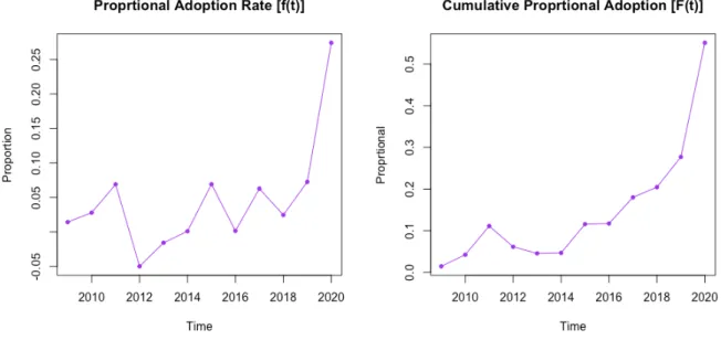
Figure 2: Historical Proportional Adoption of SPACs in relation to historical IPOs

Figure 3: Historical Adoption of SPACs

Theorem 2: 𝑎@(𝑡) = 𝑝𝑚 + (𝑝 − 𝑞)𝐴̅(𝑡) − . /𝐴̅(𝑡)

-_.

The next step of the data processing focusses on the parameter estimation that are included in the BM in order to compute the diffusion of SPAC IPOs. First, regression analysis is studied which is based on a multiple linear regression model since it may be viewed as the simpler case for parameter estimation and projections. Secondly, Bayesian analysis are applied for parameter estimation which indicate a more complex process.

The regression analysis is made with the case in section 3.2 where Theorem 2 are to be fitted through the regression analysis. The reason for choosing Theorem 2 in the regression process relate to the available data at hand and previous research by scholar utilizing similar theorem [1,3,5]. Generally, the regression process can be described to compute the parameters of BM namely, 𝑝, 𝑞 and 𝑚, trough the following steps. Firstly, the model takes the historical data presented in Figure 3 and the regression equation. The correlation with the historical diffusion of SPAC IPOs and the regression equation are thus intended to be found trough estimation of the regression with NLS as the estimation. One may highlight the importance of a “good” dataset as well as the importance to fit the proper regression equation to reduce the possibilities of large residual errors. In the case of SPAC IPOs, one may note that with the relatively few data-points for the SPAC IPOs, there is a risk of unstable values with incorrect signs in the NLS estimation which is a part of the regression analysis.

The regression coefficient that are produced are the characteristic values which through Theorem 2 can be related to the parameters in the BM. Equations (15)(16) and (17) may be used to compute the value of parameters in the BM. The model further takes these approximations of parameters from the regression process and applies them in the three

without 𝑚 which provide the theoretical Cumulative Proportional Adaptation 𝐹(𝑡), a part of each scenario. The usage of regression analysis as an estimation method for parameters are concluded with a comparison of each scenarios Cumulative Adoption 𝐴̅(𝑡) and the Cumulative Proportional Adoption 𝐹(𝑡), respectively, with historical data. The comparison is also intended to provide posterior data related to projections and the theoretical s-curve in BM.

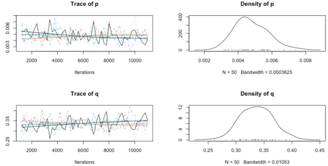
The data processing continues with the second case of analysis, parameter estimation trough a Bayesian approach. Based on section 3.3 Bayesian Bass Model in the Mathematical Background the data processing and parameter estimation follows from a simulated Bayesian bass model using Just another Gibbs sampler (JAGS). JAGS is a simulating program for Bayesian models driven by historical data. In this study the specific JAGS program is referred to as RJAGS, implying a package integrated for applications in R-studio, it is however not discussed and described in detail within this study. The data that is implemented in the created Bayesian bass model is the ratio of SPAC IPOs to the total number of IPOS each year, hence Figure 2 which shows historical Proportional Cumulative Adoption. Basically, RJAGS utilize a Markov Chain Monte Carlo simulation based on the historical data to simulate future values of diffusion. Running the Bayesian BM results in several iterations and densities of possible values for the parameters in the BM, which may be studied in section 5.2. The model consequently provides the estimated mean of the iterations for parameter values 𝑝 and 𝑞 respectively, as well as some basic statical properties to assist assessment of the estimated parameters.

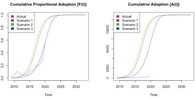
Important to note with the Bayesian BM is the absence of an estimated potential population 𝑚. Hence, one may highlight the delimitation to Cumulative Proportional Adaptation 𝐹(𝑡) in the different scenarios that follows for the estimated parameters. Similar to the previous parameter estimation method, the different scenarios are applied to compute the diffusion over a set discrete time interval with the new estimated parameter values from the Bayesian BM. The Bayesian approach does however take it a bit further, providing a superimposed plot of the Cumulative Proportional Adaptation 𝐹(𝑡) for all different iterations of parameter values in each scenario.

The concluded estimated parameter values in the two approaches are to be examined and compared to the determine the approach of preference with the more accurate estimations. The estimations can further be compared with the mean of the meta-analysis, to comprehend if the estimated values are reasonable [4]. With a preferred estimation methodology, a preferred scenario should be determined in order to state a preferred outline of modeling SPAC IPOs with the BM.

Chapter 5

5 Results

The presented proceedings in the methodology section contain two different analytical approaches of estimating the parameters and applying the BM. The first analytical approach is regression analysis where the parameters in the BM are estimated with multiple linear regression and NLS. The parameters are incorporated in the three different scenarios to compute the possible diffusion of SPAC IPOs. The implied results of the estimated parameters and graphs of the fittings in relation to the initial data are presented in each respective section below. Further the results from the second approach to estimation of parameters, namely Bayesian analysis are presented according to the same structure as the regression analysis.

5.1 Regression analysis

The regression analysis in the model provides the initial estimations of regression coefficients based on NLS estimation, presented in Table 2. The regression coefficients are to be utilized as described in section 3.2 to compute the parameters 𝑝, 𝑞 and 𝑚 presented in Table 3.

Coefficients Estimate Std. Error t Value 𝑷𝒓(> |𝒕|) 𝛽2 -1.209e+01 1.791e+01 -0.675 0.5150

𝛽3 7.272e-01 2.752e-01 2.643 0.0246*

𝛽! -5.591e-05 5.843e-04 -0.096 0.9257 Table 2: Regression coefficients

In the table above show the statistical properties of the regression coefficients in order to assist the assessment of the accuracy of the estimated BM parameters presented in Table 3. Thus, besides the mean and standard error of each regression coefficient, the t-value and Pr(> |t|) are presented with the intention to create a better understanding of the estimated coefficients. The regression coefficients may be interpreted as follows. The first, 𝛽_", has an estimate mean of -12.09 and a standard deviation of 12.91 which could be considered extremely high and further imply a poor estimation. One can further comprehend that the estimate of 𝛽_" is poor since the t-value is in close approximatively to 0 at -0.675 which can be traced to a p-value of 51.5%. Indicating that one cannot reject the null hypothesis, such that the regression coefficient is 0, and there is a fairly high probability of observing a deviating value from the mean estimate. For the second regression coefficient, 𝛽_', with a mean of 0.7272 and a standard error of 0.27, may on the other hand be considered more reliable. It is related to a t-value which is significantly larger than 0 at 2.643 which results in a p-value with a rather low probability of deviating, 2,4%, from the estimated coefficient value. We may thus reject the null hypothesis and accept the value of 𝛽_'. The last regression coefficient can on the other hand be categorized as the worst estimate. The mean estimate of 𝛽- is -0.0000559 and the standard error is 0.000584l. The t-value is thus -0.096 which is extremely close to 0 and can be interpreted as a bad approximation since there, according to the p-value, is a 92.57% probability of deviations

Parameters Estimate

𝑝 0.0009

𝑞 0.7263

𝑚 12989.82

Table 3: Regression parameters

The innovation parameter, 𝑝, is determined as 0.0009 based on the equation (16) with the mean of the regression coefficients, 𝛽", 𝛽' and 𝛽-, in equation (15). It is worth to highlight that 𝑝 is rather close to zero but above, which relate to one of the basic mathematical assumptions that follows the BM. The value is however intuitively reasonable since adopters of SPAC IPOs are unlikely to adopt by their own without any influence from others. One may also highlight the possible error that follows the parameter estimation based on the regression coefficients which again relate to equation (16) which follows:

𝑝 = U𝛽_'− k𝛽_'-− 4𝛽_"𝛽_-V 2‰ .

The main regression coefficient which impacts the estimation of 𝑝 lays outside the square root in the equation, thus β_' which is fairly accurate since PrF> Št_B4ŠG=2,4%. Thus, the estimation of 𝑝 may be considered fairly accurate. It is however important to note that the bad approximation of the first and last regression coefficients also affect the estimation of 𝑝 since these regression coefficients are included in the expression, but not to the same extent as β_'. The imitation parameter, 𝑞, is on the other hand, way above the assumption of strictly positive with a mean of 0.7263 which has been calculated on the basis of equation (17). The imitation parameter for adoption of SPAC IPOs can be considered reasonable since it means that the probability of a potential adopter to be influenced by the cumulative number of adopters is 72%. It could be considered high, but with resent large increases of SPAC adoptions it can be considered reasonable. If one study equation (17) to calculate 𝑞,

𝑞 = Uβ_'+ kβ_'- − 4β_"β_-V 2‰ ,

similarities can be found with the equation used to compute the innovation parameter. The difference is the sign in front of the square root which tend to affect the accuracy of the parameter since the error originating from the square root has a slightly different impact. However, the main correlations coefficient which affect the parameter estimation is still the same, the properties of β_' which assist the assessment of a fairly probable and reasonable value of 𝑞.

The total potential population, 𝑚, that are estimated based on the regression coefficients is on the other hand worth to highlight more extensively. In the case of SPAC IPO adoption, it is hard to assess a reasonable total number of potential adopters which could perform a SPAC IPO rather than a traditional IPO. The reasoning for this could be argued that the total number of potential adopters is a variable value since the number established unpublished firms are not constant and vary with economical state of the market. New firms are created each year and firm may go bankrupt which affect the number of potential adopters. The total potential population, 𝑚, are determined with the regression coefficients in Table 2 and Equation (15):

𝑚 = 𝑚𝑎𝑥 U−β'± kβ'-− 4β"β-V (2β‰ -).

The estimated 𝑚 reaches 12989.82. Intuitively, one may consider it to be an unreasonably large value. If one further study the approximate accuracy of 𝑚 through the statistical properties of the regression coefficient in similarity to the previous parameters. It may be obvious that the estimation of 𝑚 entail another coefficient outside of the square root which affect the accuracy. The additional regression coefficient in this case is β_- in the denominator, which is the worst estimation in the regression analysis according to Table 2 which directly affect the estimation of 𝑚. With such a small and unstable value for β_-, one can see where the large value for 𝑚 originate. The uncertainty that has been state for β_- follows, thus and creates similar uncertainties for 𝑚.

The uncertainties that follow with the regression coefficients ultimately affects the accuracy of the entire analysis of modeling SPAC IPO diffusion. In the general assessment of the regression analysis, further values which may provide an insight of the performance of the regression model is presented in Table 4Table 4: Residual errors & R-squared regression . The 𝑅-_-value for the model are interpreted provide the origin of the error. Since the 𝑅-_{-value is rather close} to 1 at 0.8688, one may conclude that the fitted regression equation, Theorem 2, provide a rather good fit and description of actual data. The residual error can thus be interpreted to represent 1-0,8688≈13.12% of the total error in the regression analysis. However, it could be important to note that since the regression error represents 86.88% of the total error, large error and uncertainties may still arise in relation to the regression coefficient and parameter estimations. Based on the p-value of the regression analysis presented in Table 4, one may further conclude that the null-hypothesis are rejected which entails that at least one regression coefficient is separated from 0 which corresponds to the parameter analysis above and the stronger statical results of 𝛽_'.

Residual standard

error

Multiple

R-squared Adjusted R-squared F-statistic on 2 and 10 DF P-value

39.2 0.8688 0.8426 33.12 3.885e-05

10 degrees of freedom

Table 4: Residual errors & R-squared regression

5.1.1 Presentation of Scenarios based on the regression analysis.

With the estimated parameters that are included in the BM, Table 3, the different scenarios of expressing the BM in a discrete time state as described in section 3.1 may be studied. The following plots shows each scenario application. Where the left-hand side refers to the a-part of each scenario and the right-hand side refers to the b-part of each scenario. The plot of the left-hand side does therefore illustrate the estimated CDF and PDF of the SPAC IPO adoption as a percentual relation to the total number of tradition IPOs each year. The right-hand side does however show the expected average cumulative number of adopters of SPAC IPOs

Figure 4: Regression fit of scenario 1a Figure 5: Regression fit of scenario 1b

Figure 6: Regression fit of scenario 2a Figure 7: Regression fit of scenario 2b

Figure 8: Regression fit of scenario 3a Figure 9: Regression fit of scenario 3b

5.1.2 Combination of all Regression Analysis Scenarios

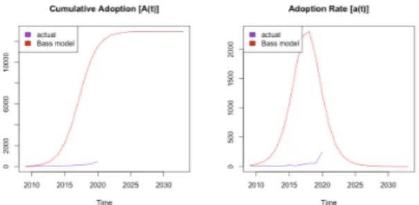
In order assist the assessment of the scenarios and their accuracy to represent the actual data based on the estimated parameters in section 5.1, Figure 10 may be constructed. The figure illustrates the combinatorial graphs of cumulative adoption of SPAC IPOs as the outcomes of applying the estimated parameters from the regression analysis with each of the three BM scenarios in combination with the actual data. On the left-hand side, the three different scenarios relate to the Cumulative Proportional Adoption fitting with the BM relying on the CDF and thus disregarding the total potential population 𝑚. The graph on the right-hand side further represents the combinatorial graph of the same scenarios, but in this instance the visualization represents the results of Cumulative Adoption which follows from fitting the b-part in each scenario based on Theorem 2, including the parameter 𝑚.

Figure 10: Regression multiplot of all scenarios

When observing the fittings on the left-hand side graph, one can argue that one scenario embarks on significance towards fitting to the actual cumulative data, this is scenario 3. Scenario 3 is an adaptation in discrete time as presented in equation (13). This scenario follows the line of the actual data in a similar manner, where the biggest differences can be observed in year 2011 and 2019. It can also be observed that scenario 1 and 2 in the same graph follow a similar pattern over the time period, where the only identified difference is that scenario 1 is offset to the right in relation to scenario 2. This can imply that this scenario will have less proportional adopters in the set time period. If one examines the equations behind these two scenarios, equation (9) and (11) respectively, it could be analyzed that they show similarities in the result because of their fundamental structures. Both of them can be portrayed as the solution to the differential equation of BM presented in equation (7) and (8) respectively. The three different scenarios should and are interpreted to show similarities since they are different ways of presenting the theorems in a discrete time format. The differences are however related to how the errors in the approximations of diffusion propagates. In hindsight scenario 3 could be assumed to show the best fitting in terms of the cumulative proportional adoption with the estimated parameters in Table 3, but does according to the mathematical background entail large propagating errors.

If one on the other hand study the right graph, it can be observed that none of the scenarios show distinctive representation of a good fit toward the historical data. The only one that somewhat can be observed to stand out is the result from scenario 3 which has a longer reaction time to climb in diffusion. Scenario 3 is not close to the actual data, but still closer than scenario 1 or 2. The large difference between the modeled diffusion with scenarios and actual data may be related to the size of the total potential population 𝑚 which is an unstable estimate due to the impacts by the last regression coefficient in the computation. The estimate could be considered to be ridiculously large in comparison with historical rate of change from year to year which may be observed in Table 1.