DISTRICT HEAT PRICE MODEL
ANALYSIS
A risk assessment of Mälarenergi’s new district heat price model
ERIK LANDELIUS
MAGNUS ÅSTRÖM
School of Business, Society and Engineering
Course: Degree Project Course code: ERA403 Credits: 30HP
Program: Master Engineer – Energy systems
Supervisor (MDH): Allan Hawas Supervisor (Mälarenergi): Einar Port Examiner: Erik Dahlquist
Customer: Mälarenergi Date: 2019-06-07 Email:
mam10002@student.mdh.se els14001@student.mdh.se
i
ABSTRACT
Energy efficiency measures in buildings and alternative heating methods have led to a decreased demand for district heating (DH). Furthermore, due to a recent increase in extreme weather events, it is harder for DH providers to maintain a steady production
leading to increased costs. These issues have led DH companies to change their price models. This thesis investigated such a price model change, made by Mälarenergi (ME) on the 1st of August 2018. The aim was to compare the old price model (PM1) with the new price model (PM2) by investigating the choice of base and peak loads a customer can make for the
upcoming year, and/or if they should let ME choose for them. A prediction method, based on predicting the hourly DH demand, was chosen after a literature study and several method comparisons were made from using weather parameters as independent variables.
Consumption data from Mälarenergi for nine customers of different sizes were gathered, and eight weather parameters from 2014 to 2018 were implemented to build up the prediction model. The method comparison results from Unscrambler showed that multilinear
regression was the most accurate statistical modelling method, which was later used for all predictions. These predictions from Unscrambler were then used in MATLAB to estimate the total annual cost for each customer and outcome. For PM1, the results showed that the flexible cost for the nine customers stands for 76 to 85 % of the total cost, with the remaining cost as fixed fees. For PM2, the flexible cost for the nine customers stands for 46to 61 % of the total cost, with the remaining as fixed cost. Regarding the total cost, PM2 is on average 7.5 % cheaper than PM1 for smaller customer, 8.6 % cheaper for medium customers and15.9 % cheaper for larger customers. By finding the lowest cost case for each customer their optimal base and peaks loads were found and with the use of a statistical inference method (Bootstrapping) a 95 % confidence interval for the base load and the total yearly cost with could be established. The conclusion regarding choices is that the customer should always choose their own base load within the recommended confidence interval, with ME’s choice seen as a recommendation. Moreover, ME should always make the peak load choice because they are willing to pay for an excess fee that the customer themselves must pay otherwise.
Keywords: district heating, multilinear regression, Bootstrapping, Mälarenergi, weather
parameters, heat prediction, statistical inference, Unscrambler
Nyckelord: fjärrvärme, multilinjär regression, Bootstrapping, Mälarenergi,
ii
PREFACE
This thesis was conducted under the auspices of the Energy Systems programme at Mälardalen University. The division of labour was split even and fair, where each person’s strength was utilized to the best of their abilities. We, the authors, would like to thank
Mälarenergi for accepting the thesis draft early on and for providing assistance and necessary data, without which this report would have been difficult to write. Especially big thanks to Einar Port, who was our supervisor at Mälarenergi.
We also wish to express our gratitude to Bostads AB MIMER for giving us access to view their customer’s district heat consumption through Mälarenergi.
Furthermore, we would like to thank the following professors and doctorate students at Mälardalen University, who kindly answered our questions and guided us on the right path: Jan Skvaril, assistant professor in Energy and Environmental Engineering
Karl Lundengård, teacher and doctorate student in applied mathematics at Mälardalen University
Christopher Engström, teacher and doctorate student in applied mathematics at Mälardalen University
An additional thanks to Fredrik Karlsson at SMHI who informed us and recommended different prediction methods.
Västerås 7th of June 2019
Erik Landelius
Magnus Åström
If I have seen a little further, it is by standing on the shoulders of Giants.
iii
SUMMARY
Anthropogenic climate change has caused a shift in the political climate towards
environmentally friendly energy solutions. Sweden is actively contributing to this goal and its heating market has seen a rise of new energy efficient heat pumps that are competing with the more seasoned district heating (DH) technology, which currently holds 50% of the heating market share. DH rose to prominence in Västerås with Mälarenergi (ME); a municipally owned company that operates several combined heat and power plants, from which heat is co-generated during electricity generation and distributed in a system of pipes to the end-users.
Lately, due to more energy efficient buildings and alternative heating methods, the demand for DH has decreased. Moreover, due to recent extreme weather it is harder for DH providers to maintain a steady production, leading to increased costs. These issues have led DH
companies to change their district heat price models. ME introduced their new price model on the 1st of August 2018 for its larger customers, but not for private customers. This new price module is based on the customer’s choice of base and peak load for their heat demand. The old Mälarenergi price model for private customers had a yearly fixed cost independent of the customer’s size, and a variable cost that depended on the season.For companies the old price model had a fixed cost that depended on connected loads.
Predicting the heat demand is essential for power plants to use their resources optimally. These predictions are essentially weather forecasts but include demand-side information as well. There are three forecasting classifications mainly used by researchers today: machine learning methods, physical methods and statistical methods. This report limits itself to only analyzing statistical methods for prediction purposes.
The aim of this report is to compare the old and the new DH price model and investigate what choice of base and peak loads a customer should make for the upcoming year, or if they should let ME choose. A forecasting method will also be chosen to predict the heat demand using weather parameters, and from this heat demand the costs will be calculated.
The method started with a literature study to research old and new DH price models,
especially the ones ME have. Modelling methods were investigated similarly, and teachers at MDH were contacted for further guidance about mathematics and choice of software. From ME, DH consumption data of nine different customers (sorted in load size as three small, three medium and three large) were gathered as well as weather data. The software used for modelling and calculations were MATLAB, Excel and Unscrambler.
Unscrambler was used to predict the DH demand from weather parameters. A training set of five years of weather data, given from ME, was used to build the prediction model. Later, to avoid creating weather forecasts, ten years of weather data from an SMHI database of Stockholm was used to create a probability distribution of possible weather events. These years of weather data were used to predict the corresponding heat demand for customers of
iv
ME. The heat demand data were then imported to MATLAB to calculate the costs of the old and new DH price models. Excel was used for organizing, storing and visualising of all data. The Bootstrap method was used on the predicted yearly cost and optimal base load which stems from the new weather data, with the main purpose of inferring information about the whole population.
The most accurate statistical modelling method in Unscrambler was multilinear regression (MLR), which was better than partial least square regression (PLS) and principal component (PCR) regression for small, medium and large customers. The results also showed that weather data on an hourly basis could not predict the consumption as accurately as weather data on a daily basis. On average the hourly r-square value fluctuated between 70 - 84% while the daily r-squared fluctuated between 90 – 94 %
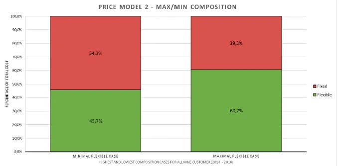
For price model 1, the results showed that the flexible cost for the nine customers accounted for 76 to 85 % of the total cost, and the rest was fixed cost. For price model 2, the flexible cost for the nine customers accounted for 46 to 61 % of the total cost, and the rest was fixed cost. For the total cost, PM2 was on average 7.5 % cheaper than PM1 for smaller customer, 8.6 % cheaper for medium customers and 15.9 % cheaper for larger customers.
The expected optimal base load was calculated with a 95% confidence interval for each customer, which was based on ten different weather scenarios. The deviation in mean total cost from the theoretical minimum mean cost ended up around 2%, which was calculated by choosing the base loads corresponding to the 95 % confidence intervals limits.
For the results to be more statistically accurate and scientifically reliable, many more weather samples should have been used, and not just ten years of data from one city. We first focused on a single sample to produce satisfying results which would then be repeated with a much larger sample and inferred on the population. However, due to time limitations, a larger sample could not be studied. This is of course a source of error and as a suggestion for further work we propose replicating this study whilst adding more weather data samples. To make it even more accurate, another suggestion is implementing weather forecasts a few weeks ahead in time. With these forecasts, a customer’s consumption can be predicted with an attached cost. Later, this forecast can be verified with the actual weather data of that time period to test the accuracy of the prediction model.
By finding the lowest cost case for each customer their optimal base and peak loads were found and with the use of a statistical inference method (Bootstrapping) a confidence interval for the base load and total yearly cost with 95% confidence could be established. The
conclusion regarding choices is that the customer should always choose their own base load within the recommended confidence interval, with ME’s choice seen as a recommendation. Moreover, ME should always make the peak load choice because they are willing to pay for an excess fee that the customers themselves must pay otherwise.
v
SAMMANFATTNING
Klimatförändring orsakad av mänskliga faktorer har skapat en förändring i det politiska landskapet mot mer miljövänliga energilösningar. Sverige tar aktivt del i denna politik och effektiva värmepumpar har slagit igenom stort i den inhemska värmemarknaden, som domineras av fjärrvärme (FV), vilket håller 50 % av marknadsandelen. FV:s framgång i Västerås beror på kommunalägda Mälarenergi, vilket driver kraftvärmeverk som genererar el och FV samtidigt till sina kunder.
På senaste tiden har efterfrågan efter FV minskat, på grund av energieffektivare byggnader och alternativa uppvärmningsmetoder. Utöver detta har extrema väderförhållanden gjort det svårare för FV-bolag att hålla en stadig produktion, vilket lett till ökade kostnader. Dessa problem har lett FV-bolag till att förändra sina FV-prismodeller. Mälarenergi introducerade sin nya FV-prismodell den 1:a augusti 2018 för större kunder (ej privata). Denna prismodell är baserad på kundens val av bas- och topplast för deras värmebehov. Den äldre
prismodellen för private kunder hade en årlig fast kostnad oberoende av kundens storlek och en rörlig kostnad beroende på årstid. För stora fastigheter och grupphusområden berodde den fasta kostnaden på ansluten effekt.
Att förutspå värmebehovet är viktigt för att kraftvärmeverk ska utnyttja sina resurser optimalt. Dessa prediktioner är i grund och botten väderprognoser men innehåller även information från kundens sida. Det finns tre klassifikationer för de prediktioner som används mest, dessa är: maskininlärningsmetoder, fysiska metoder och statistiska metoder. Denna rapport begränsar sig till att endast undersöka statistiska metoder.
Målet med denna rapport är att jämföra den äldre och den nya FV-prismodellen och undersöka vilket val av bas- och topplast en kund ska göra för nästkommande år, eller om Mälarenergi ska göra valet åt kunden. En prediktionsmetod ska väljas för att prediktera fjärrvärmebehovet med hjälp av väderparametrar, och från detta behov beräknas årskostnaderna.
Metoden började med en litteraturstudie för att undersöka äldre och nya FV-prismodeller, speciellt dem Mälarenergi har. Modelleringsmetoder undersöktes på liknande sätt och professorer på MDH kontaktades för ytterligare vägledning om matematik och val av mjukvara.
Från Mälarenergi erhölls konsumtionsdata över kunderna och väderdata. Mjukvaran som användes för modellering och beräkningar bestod av MATLAB, Excel och Unscrambler. Unscrambler användes för att prediktera värmebehov utifrån väderparametrarna. Ett träningsset på fem år av väderdata från Mälarenergi användes för att bygga upp
prediktionsmodellen. Därefter, för att undvika att behöva skapa egna väderprognoser, togs 10 år av väderdata från SMHI över Stockholm för att skapa ett utfall av möjliga
väderförhållanden. Dessa år med väderdata användes för att prediktera motsvarande värmebehov för Mälarenergis kunder. Datamängden över värmebehovet exporterades till
vi
MATLAB där kostnaderna för dem två prismodellerna beräknades. Excel användes för att organisera och strukturera datamängden, men även senare för att visualisera resultaten med tabeller och diagram. Bootstrap-metoden användes på predikterad årlig förbrukning och optimala baslaster, vilka hade sitt ursprung i nya väderparametrar, för att estimera information på hela populationen.
Den noggrannaste statistiska modelleringsmetoden i Unscrambler var multilinjär regression (multilinear regression), vilket var bättre än partiell minstakvadratmetoden (partial least square regression) och principiell komponentregression (principal component regression) för små, medium och stora kunder. Resultaten visade också att väderdata på timbasis inte kunde prediktera konsumtion lika noggrant som väderdata på dygnsbasis kunde. I genomsnitt låg den timbaserade determinationskoefficienten (r2) mellan 70 – 84 % och den dygnsbaserade mellan 90 – 94 %.
För prismodell 1 visade resultaten att den rörliga kostnaden för de 9 kunderna stod för 76 till 85 % av den totala kostnaden, varav resten var fast kostnad. För prismodell 2 stod den rörliga kostnaden för 46 till 61 % av totalkostnaden, varav resten var fast kostnad. För den totala kostnaden visade resultatet att PM2 i genomsnitt var 7,5 % billigare än PM1 för små kunder, 8,6 % billigare för mediumkunder och 15,9 % billigare för större kunder. Den förväntade optimala baslasten beräknades med ett konfidensintervall på 95 % för varje kund, baserat på tio olika väderscenarier. Avvikelsen i genomsnittskostnaden från den teoretiskt minimala genomsnittskostnaden var runt 2 %, vilket beräknades genom att välja baslasterna som föll inom ramen av konfidensintervallet på 95 %.
För att resultaten ska vara mer statistiskt noggranna och vetenskapliga behövdes flera
väderurval för att kunna dra exakta slutsatser om populationen. I rapporten användes endast 10 år av väderdata från Tullinge. Vi behövde först fokusera på ett enda urval och se till att vi kunde producera ett resultat vi var nöjda med vilket skulle upprepas på ett större urval för att dra slutsatser på populationen. Dock, på grund av tidsbegränsningen, kunde inte ett större urval undersökas. Detta är såklart en felkälla och som förslag på fortsatta studier föreslår vi att studien upprepas med ett större urval av väderdata. Ett annat intressant förslag är att lägga till faktiska väderprognoser några veckor fram i tiden. Med dessa prognoser kan en konsumtion beräknas med en motsvarande kostnad. Därefter kan denna prognos verifieras med den datamängden som faktiskt uppmättes för vädret, för att testa noggrannheten på prediktionsmodellen.
Genom att hitta den lägsta kostnaden för varje kunds förbrukning kunde den optimala bas- och topplasten utvinnas, och med hjälp av bootstrapping kunde ett 95 % konfidensintervall konstrueras kopplat till val av baslast och kostnad. Slutsatserna kring val av last är att kunderna alltid bör välja baslast inom det rekommenderade konfidensintervallet, med ME:s val som en vägledning. Dessutom bör ME alltid sätta topplasten åt kunden eftersom då undviker kunden att behöva betala en överuttagsavgift om de hade gjort valet på egen hand.
vii
CONTENT
1 INTRODUCTION ...1
1.1 Background ... 1
1.1.1 Environmental context ... 1
1.1.2 Mälarenergi - The district heat provider ... 2
1.1.3 Predicting the heating demand ... 3
1.2 Purpose ... 4
1.3 Research questions ... 4
1.4 Delimitation ... 5
1.4.1 Multivariate modelling delimitations ... 5
1.4.2 Data gathering delimitations ... 5
1.4.3 Price model delimitations ... 6
1.4.4 Meteorological delimitations ... 6
1.5 Thesis structure ... 7
2 METHOD ...8
2.1 Ethics and methodology ... 8
2.2 Literature study and interviews ... 9
2.2.1 District heat ... 9
2.2.2 Multivariate and statistical analysis ... 9
2.3 Gathering of the empirical data ...10
2.4 Modelling and analyzing software ...10
2.4.1 The Unscrambler ...10
2.4.2 Excel ...10
2.4.3 MATLAB ...11
3 LITERATURE STUDY ... 12
3.1 A short summary of how district heat works...12
3.2 A new phase for district heat ...13
3.3 A general description of DH price models ...14
viii
3.4.1 Price model 1 (PM1) ...17
3.4.2 Price model 2 (PM2) ...17
3.4.3 Difference between PM1 and PM2 ...19
3.5 Degree days ...19
3.6 Multivariate modelling/analysis/statistics ...20
3.6.1 Statistical methods ...20
3.6.2 Linear regression ...21
3.6.2.1. LINEAR REGRESSION TERMINOLOGY ... 21
3.6.3 Statistical model validation methods ...23
3.6.3.1. SIMPLE LINEAR REGRESSION (SLR) ... 25
3.6.3.2. MULTIPLE LINEAR REGRESSION (MLR) ... 26
3.6.4 Principal Component Analysis (PCA) ...27
3.6.5 Principal component regression (PCR) ...28
3.6.6 Partial least square regression (PLS regression) ...28
3.6.7 Bootstrapping ...29
3.6.8 Optimal amount of independent variables when predicting heat demand ...30
3.6.9 Sample size considerations for regression models ...31
3.7 Center and scale ...32
4 CURRENT STUDY ... 33
4.1 Gathering of data ...33
4.2 Unscrambler method ...33
4.2.1 The general Unscrambler modelling routine ...33
4.2.2 Choosing the right modelling method: MLR, PCR or PLS ...34
4.2.3 Number of weather parameters to use ...35
4.3 MATLAB Modelling ...35
4.3.1 Part 1 – User input and metadata...36
4.3.2 Part 2 - Import and data handling ...36
4.3.3 Part 3 – Price model 1&2 ...36
4.3.3.1. PRICE MODEL 1 ... 36
4.3.3.2. PRICE MODEL 2 ... 36
4.3.3.3. PM1 VS PM2 ... 38
ix
4.3.5 Part 5 – Export results ...38
4.4 Bootstrapping ...38
4.4.1 Further calculations regarding confidence intervals ...38
5 RESULTS WITH CLARIFICATION ... 40
5.1 Gathered data and price model 1 & 2 ...40
5.1.1 Consumption and weather data ...40
5.1.2 Price model 1 ...43
5.1.3 Price model 2 ...45
5.1.4 Validation ...48
5.2 PM1 versus PM2 ...49
5.3 Multilinear Regression & Unscrambler Results ...50
5.3.1 Choosing the right method: MLR, PCR or PLS...50
5.3.2 Analyzing MLR ...53
5.3.3 Number of weather parameters to use ...55
5.4 Bootstrapping ...56
5.4.1 Excel: Bootstrap ...56
5.4.2 Statkey: Bootstrap ...56
5.4.3 Prediction results analysis ...58
6 DISCUSSION... 64
6.1 Sources of errors ...64
6.2 Additional thoughts ...66
7 CONCLUSIONS ... 70
8 SUGGESTIONS FOR FURTHER WORK ... 71
REFERENCES ... 72
APPENDIX 1: GRANT FROM MIMER AB ...1
APPENDIX 2: MACHINE LEARNING ...2
x
APPENDIX 4: MATLAB CODE ...4
APPENDIX 5: EXCEL DATA STRUCTURE ... 10
APPENDIX 6: ADDITIONAL WEATHER PARAMETERS ... 11
APPENDIX 7: CUSTOMER INVOICE ... 12
LIST OF FIGURES
Figure 1 Illustration of the PLS process ... 29Figure 2 Daily temperature and degree days in Västerås 2014 ... 40
Figure 3 Customer 1: Daily temperature and consumption in Västerås ...41
Figure 4 Customer 4: Daily temperature and consumption in Västerås ... 42
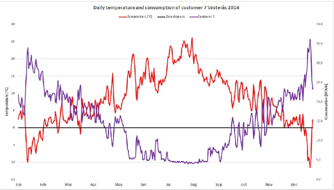
Figure 5 Customer 7: Daily temperature and consumption in Västerås... 42
Figure 6 Total fixed cost curve vs Initial tangent for PM1 ... 43
Figure 7 PM1: Fixed and flexible costs ... 44
Figure 8 PM1: Max/min of fixed and flexible ... 44
Figure 9 Finding the minimum total cost for customer 1 ... 45
Figure 10 Total fixed costs vs Initial tangent (PM2) ... 46
Figure 11 PM2: Fixed and flexible costs ... 47
Figure 12 PM2: Max/min of flexible and fixed costs ... 48
Figure 13 PM1 vs PM2: Flexible and fixed costs ... 49
Figure 14 PM1 vs PM2: Total cost ... 50
Figure 15 t-values Customer 1 ... 54
Figure 16 Predicted vs. Reference values ... 54
Figure 17 Bootstrap in Excel for customer 1... 56
Figure 18 Bootstrap annual cost result from StatKey customer 1 ... 57
Figure 19 Bootstrap Base load result from StatKey customer 1 ... 57
Figure 20 Customer 1 Optimal base load choice with corresponding cost ... 59
Figure 21 Visualization of the normal distribution and confidence interval for customer 1 ... 59
Figure 22 Additional cost in relation to the theoretical optimum ... 60
Figure 23 Additional cost in relation to the theoretical optimum (Customer 1) ... 60
Figure 24 Predicted total annual cost (Customer 1) ...61
Figure 25 Extra cost when deviating from expected optimal base load (Customer 1)...61
Figure 26 Extra cost when deviating from expected optimal base load (Customer 4) ... 62
xi
LIST OF TABLES
Table 1 Steps of the thesis process ... 8
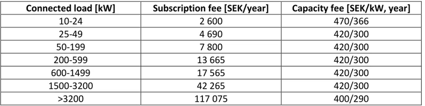
Table 2 Fixed fee PM1 for large properties and group connected houses ... 17
Table 3 Variable fee PM1 for large properties and villas ... 17
Table 4 Fixed fee PM2. Large properties/group connected houses ... 18
Table 5 Variable fee PM2 ... 18
Table 6 Overview of DH price components between PM1 and PM2 ...19
Table 7 Linear regression terminology ... 22
Table 8 Different definitions of Sum of Squares ... 22
Table 9 Mean square and standard regression definitions ... 23
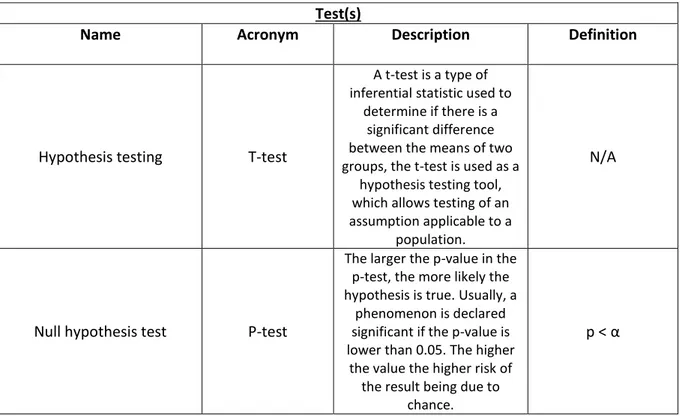
Table 10 Validation parameters/Tests ... 24
Table 11 Table of coefficients ... 25
Table 12 Error margin as a function of degrees of freedom ... 32
Table 13 Daily and hourly consumption correlation to temperature ... 43
Table 14 Base vs Peak load (Medium customers) ... 46
Table 15 Base vs Peak load (Small customers) ... 46
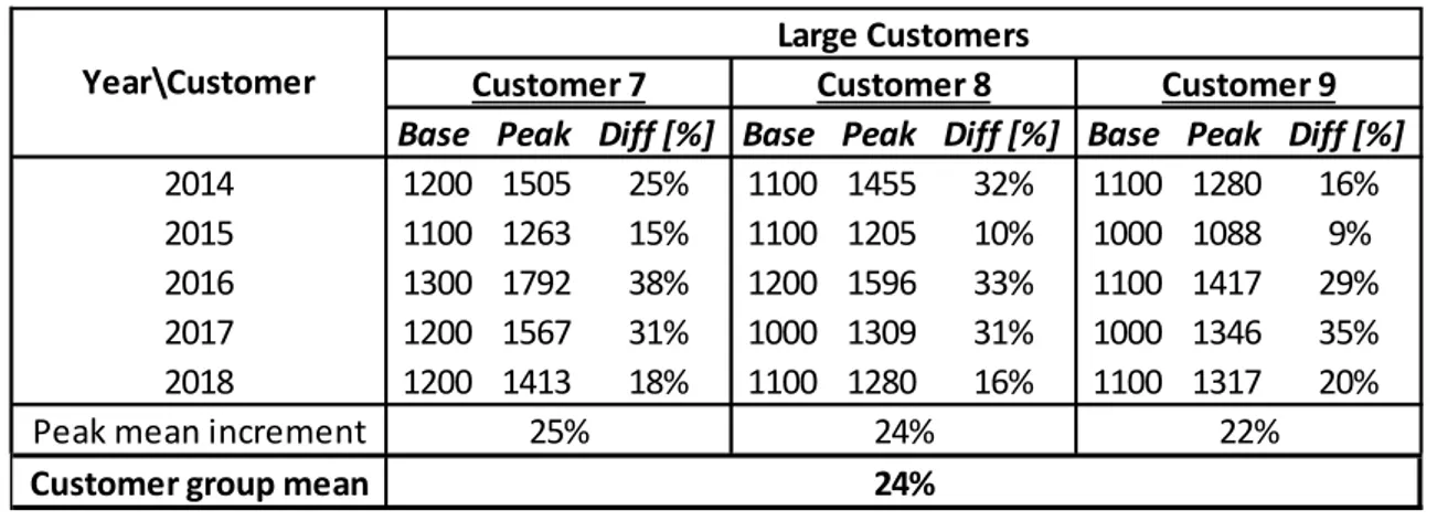
Table 16 Base vs Peak load (Large customers) ... 47
Table 17 Difference between base and peak load regarding ME's choice ... 47
Table 18 PM2 cost validation ... 48
Table 19 PM1 vs PM2 ... 50
Table 20 Method comparison of Customer 1 in 2018 ... 51
Table 21 Method comparison of customer 4 in 2018 ... 51
Table 22 Method comparison of customer 7 in 2018... 51
Table 23 Method comparison of three customers in 2015 ... 52
Table 24 Anova Table for Customer 1 ... 53
Table 25 Number of weather parameters ... 55
Table 26 Coefficient of determination ... 55
Table 27 Bootstrap confidence interval results for base load and annual cost ... 58
Table 28 Deviation from expected optimum for base load and annual cost ... 58
xii
NOMENCLATURE
Symbol Description Unit
C Velocity m/s E Energy [MWh] P Power/Load [kW] t Time [h] T Temperature [°C] V Volume [m3]
r2 (or R2) Coefficient of determination [ - ] r (Pearson) Correlations coefficient (Pearson’s) [ - ]
ABBREVIATIONS
Abbreviation Description
ANN Artificial Neural Network
CHP Combined Heat and Power
DH District Heat
kW Kilowatt
kWh Kilowatt hour
ME Mälarenergi
MM Millimetres (milli)
MBAR Milli bar
MDH Mälardalen University MLR Multiple Linear Regression PCA Principal component analysis PLSR Partial least squared regression
SEK Swedish krona
SMHI Swedish Meteorological and Hydrological Institute TSR Time series regression
xiii
DEFINITIONS
Definition Description
A posteriori Experience-based knowledge. Denoting reasoning or knowledge which proceeds from observations or experiences to the deduction of probable causes. Descriptive
statistics Helps describe, show or summarize data in a meaningful way. This limits the method to only describe and/or draw conclusion about the gathered dat. This means that descriptive statistics is not developed on the basis of probability theory, unlike inferential statistics.
Deterministic A deterministic system or model is one in which no randomness is involved, meaning that it will produce the same result under the same conditions.
Empirical Information collected that is provable or verifiable by experience or experiment.
Epistemology A branch of philosophy concerned with the theory of knowledge. Or the study of the nature of knowledge, justification, and the rationality of belief.
Iff If and only if
Inference
statistics Uses a random sample taken from a limited number of outcomes or a population to describe and make inferences about the whole population. Inferential statistics are valuable when knowledge of all possible outcomes is not possible or an when examination of an entire population is not convenient or possible. Isomorphism An isomorphism is a map that preserves sets and
relations among elements. The word is derived from the Greek iso, meaning “equal”, and morphism, meaning “to form or to shape”.
Price model 1
(PM1) The 2017 DH price model for businesses Price model 2
(PM2) The 2019 DH price model for businesses Statistical
model A statistical model is based on collected empirical data, often in large quantities, for the purpose of inferring proportions in a whole from those in a representative sample. Its main purpose is analysing stochastic variables and their probability
distributions to describe the behaviours of a studied object.
1
1
INTRODUCTION
The main purpose of this report is to present to the customers of Mälarenergi’s (ME) new district heat (DH)price model what an active choice of base and peak load entails, for the following year. The aim is to accomplish this by performing a risk assessment on the customer’s choice of loads, utilizing their DH consumption and eight weather parameters (rain intensity, wind speed, wind direction, wind gust, rainfall, relative humidity,
atmospheric pressure and outside temperature). The customer’s weather conditions for the upcoming year will be extracted from previously measured weather data, which will be seen as different future cases i.e. plausible outcomes. From these outcomes the DH consumption will be predicted based on how the consumption relates to the weather conditions. A
literature study about Mälarenergi’s price models, multivariate regression modelling and DH in generalwill be conducted to complement the research.
1.1 Background
Investigating this DH price model is beneficial for the customers as it creates an incentive to be more energy efficient because of the economic benefit to be had, which in turn lowers the total energy consumption in the region. Consequently, the Swedish climate goals can be reached sooner. Since this DH price model is not even a year old (it was released in august 2018) and due to its complicated nature, this thesis aims to help customers make informed choices regarding their heat consumption. From this knowledge the customers also have a chance to understand how their DH consumption affects their costs and adapt accordingly if possible. Finally, this report aims to demonstrate how weather parameter variations correlate to the heat consumption of DH users. This knowledge can further help customers optimize their consumption patterns and create a foundation for future studies in energy efficiency improvements.
1.1.1 Environmental context
The consensus among researchers is that the climate is changing (meaning change unlike predicted patterns from observed empirical data) and the cause is believed to be
anthropogenic (man-made) (Cook et al., 2013). This has led to climate change taking a vital part in the current political climate. According to the United Nations (2016), climate change is a persisting challenge that governments and global organizations are continuously trying to counteract. The Intergovernmental Panel on Climate Change (IPCC) announced in October 2018 that after the 1.5°C global warming mark, adverse impacts of climate change will happen. In order to not reach the 1.5°C mark however, profound and rapid changes are required in all areas of society.
2
The long-term climate goal in Sweden is to reach net emissions of zero by 2045, meaning the emissions put out should not exceed the emissions removed. In order to reach this goal, different stages have been announced by the Swedish government, such as decreasing the emissions from the non-commercial sector by 40 % until 2020 (compared to 1990) and decreasing the domestic transportation emissions by 70% until 2030 (compared to 2010), according to Naturvårdsverket (2018).
Heat demand is most common in areas such as industry, agriculture, residential living and facilities. Manufacturing processes in the industry sector can require heat to be very hot, such as in glass, steel or paper manufacturing. Maintaining a comfortable inside temperature is also of importance in these facilities, which is also true for residential houses, especially during the colder months of the year. Heat is also needed in houses to heat up tap water. In the agriculture sector, heat is needed to dry crops and to heat up animal stables. All these different heating demands are usually met using fuels in nearby boilers. Therefore, the heating market is closely related to the fuel market. When district heating is used, it is delivered in competition with any fuels the customer is using in their own boiler, if they have one. (Frederiksen & Werner, 2014)
The Swedish heating market has for the last 40 years been increasing as a result of a higher heat demand. However, as heating methods and buildings are becoming more energy efficient, because of ambitious sustainable development goals, the increase is slowing down and therefore Sweden could potentially face a decreasing heat demand. Mainly, four different technologies are competing for the heating market, these are: biofuel boilers, electric heating, heat pumps and district heating. Energy wise the district heating holds more than 50% of the heating market share. This means that the district heating market is easily affected by a warmer climate and improved energy solutions which would make the customers more energy efficient. (Sköldberg & Rydén, 2014)
District heating (DH) is considered to be both environmentally sustainable and cost-effective and as such, it has become the common heating method in Sweden. The reason behind these benefits stems from how district heat is generated. Otherwise wasted resources, such as waste (both domestic and foreign) and waste heat from industrialized processes are used to generate heat (in the form of hot water) that is distributed in a system of pipes to heat up the end-user’s facilities. (Song, 2017)
1.1.2 Mälarenergi - The district heat provider
Mälarenergi is a company owned by the municipality of Västerås that provides district heating to local households and commercial buildings, from several combined heat and power plants. These plants consist of five different boilers that run on different fuels and in 2020, a new boiler and turbine will be installed that align with Mälarenergi’s own goals for sustainable development. This new boiler and turbine will be fueled by recycled wood, making all five facilities independent of fossil fuels and instead only renewable or recycled fuels will be used. (Mälarenergi, 2019b)
3
Mälarenergi uses the boiler with the lowest operating cost as a base load, which is fueled by waste and biofuel. Peak loads are covered by more expensive fuels and plants. As events of extreme weather occurs more frequently the heat demand becomes more volatile, which increases the temporary usage of the peak boilers and thus increasing their emissions and costs. Users opting for another way to obtain heat is another issue for district heating companies like Mälarenergi. Heat pumps have become popular lately due to how energy efficient they have become and because they allow users to lower their cost for heating by adapting to the electricity price, which is controlled by the market and not set on a yearly or seasonal basis by the district heating company. (Song, 2017)
To remain viable and competitive on the market, multiple district heat companies, including Mälarenergi, have changed their pricing modules to give the customer more ways to influence their total cost (Song, Li, & Wallin, May 1, 2017a). Mälarenergi introduced their new price model on the 1st of august 2018 for its larger customers, such as apartment complexes and commercial buildings, and not for private customers (Mälarenergi, 2018b). This new price module is based around the customer’s choice of base and peak load for their heat demand. But if the customer exceeds their chosen peak load, they will have to pay an excess fee, which makes the customer's choice a financial risk on their behalf. Mälarenergi motivates this excess fee by stating that it gives customers incentive to save energy when it is very cold outside, thus reducing the need from Mälarenergi to fire up peak boilers with a higher production cost and greater climate impact compared to the base load boiler. Although, Mälarenergi will suggest a base and peak load to the customers and if they agree to these pre-determined loads there will be no excess fee for overconsumption, thus reducing the
customer’s risk. This new price model also means that the cost increases for customers with a higher heat demand. The old Mälarenergi price model had a yearly fixed cost independent of the customer’s size, and a variable cost that depended on the season. For villas this old price model is still active, but for larger customers the fixed fee is based on connected loads (Mälarenergi, 2017).
1.1.3 Predicting the heating demand
In order to optimally use the available resources from a power plant it is essential that the demand-side is predicted accurately. This prediction includes forecasting weather
parameters and demand-side information, such as number of occupants (Saloux &
Candanedo, 2018). In fact, buildings in Europe account for 40% of the total energy usage. Predicting the energy consumption from buildings has therefore become important, and the method used to predict has changed as well, from calculating the energy consumption to real-time monitoring using analyzed and measured data (Jovanović, Sretenović, & Živković, 2015).
A study conducted byLazos, Sproul and Kay (2014) reviewed different methods of predicting energy demand by using weather forecasts. They generalized that there are three forecasting classifications; machine learning methods, physical methods and statistical methods, and that hybrids between them exist to complement each other. They found that statistical approaches are easy to implement, yield short simulation times and they do not require
4
intense calculating power. Examples of statistical techniques are: Multiple Linear Regression (MLR) (Tiryaki & Aydın, 2014), PCR and PLS. The drawbacks with statistical techniques are that they depend on consistent historical data when solving non-linear problems and they have a difficult time interpreting such non-linear relationships. For this reason, machine learning techniques are recommended as an alternative because they are better at solving non-linear relationships. Nonetheless, Lazos et al (2014) mentioned that machine learning algorithms are complicated and computationally intense, yet they still rely on consistent and reliable historical data. Overfitting to the datasets is another issue with machine learning. The most commonly used machine learning techniques are: Artificial Neural Networks (ANN), Support Vector Machines (SVM) and Decision Trees (DT) (Saloux & Candanedo, 2018). Physical methods are about physically interpreting the relationships between the input and output variables, or as Lazos et al (2014) put it, analyzing the hidden yet critical principles that control the system. This means using mathematics to model a physical process to forecast a future state. Physical models are often hard to estimate accurately and often simplifications are made, which of course makes the results less credible. (Lazos et al., 2014)
1.2 Purpose
The main goal with this report is to present a deeper understanding and insight about Mälarenergi’s new district heat price model to its customers, which will include what their choice of base and peak load entails. This will be achieved by analyzing and modelling the correlation between weather conditions and the DH consumption.
1.3 Research questions
What method of multivariate data analysis is most appropriate and accurate when using previous DH consumption and weather conditions to predict future DH consumption?
How should a customer choose their base and peak loads for the upcoming year in the new DH price model?
Which of the two Mälarenergi DH price models is the most profitable and how does the customer size affect the profitability?
5
1.4 Delimitation
The delimitations are split into the four different subtitles: multivariate modelling, data gathering, price model, and meteorological delimitations.
1.4.1 Multivariate modelling delimitations
All three forecasting classifications mentioned in 1.1.3 Predicting the heating demand (i.e. machine learning methods, physical methods and statistical methods) will not be studied, mainly due to time and knowledge limitations. Instead the focus will only be on statistical methods, since the authors of this thesis are most familiar with statistical methods, especially linear regression.
Machine learning methods were mentioned by several teachers (Engström, 2019;
Lundengård, 2019; Skvaril, 2019) as being computationally demanding and time consuming, moreover the authors lack basic knowledge of the principals behind machine learning
methods.
For a physical method to work, a house needs to be modelled physically, such as the dimensions and heat transfer coefficient of the walls and windows. This is a method SMHI uses, according to Karlsson (2019) who is an employee at SMHI. Karlsson did not
recommend physical method since sufficient knowledge is missing about the houses or buildings for this project, apart from the DH consumption. Instead he recommended statistical methods.
1.4.2 Data gathering delimitations
The consumption data will exclusively be obtained from ME on an hourly basis. The authorization for this was granted by the housing company Mimer AB, after asking for permission to investigate their customers’ DH consumption. This authorization can be seen in Appendix 1: Grant from mimer AB.A geographical delimitation will be that only district heat data from customers of Mälarenergi in the county of Västmanland will be investigated. The same goes for meteorological data; all of it will be gathered by Mälarenergi from the Västmanland region. The weather data given from Mälarenergi consisted of the following eight variables: rain intensity [mm/h], wind direction [degrees], rainfall [mm], relative humidity [%], atmospheric pressure [mbar], wind speed [m/s], wind gust [m/s], outside temperature [°C]. The time period in which data is received goes from 2010-01-01 to 2019-03-10. However, a lot of weather data between 2010 and 2012 is invalid (no measurements), thus no data sooner than 2012 will be used from Mälarenergi.
The consumption data from Mälarenergi for the nine customers was gathered between 2014 to 2018. This limited the model’s sample size to data from 2014 to 2018, instead of 2012-2018 from which weather data was obtained.
Leap year dates will not be considered. To get accurate data for a day that occurs so rarely, once every fourth year, many more years of data is needed, or rather, a lot of leap year data is
6
needed. The extra work and data needed for just one day was deemed not worthwhile, especially due to time limitations.
1.4.3 Price model delimitations
An important delimitation for the customer is how strong the correlation coefficient is between the weather conditions and the customer’s DH consumption. Specifically, the degree days are considered for this delimitation of customers. If the correlation between the degree days and a customer’s DH consumption of the same time period is below 90%, the correlation is not strong enough, and the customer’s DH consumption cannot be accurately predicted.
This thesis will only look at past and present DH price models developed by Mälarenergi. The present DH price model (PM2) refers to the one introduced on the 1st of august of 2018 for their larger customers and the past model (PM1) refers to the one that predated the new one. Both price models will be further explained in the literature study.
Irregularities and deviations in the price model itself will not be considered. This means deviations such as inflation or annual price adjustments made by Mälarenergi themselves or similar alterations.
No customer is assumed to have a larger baseload than 3 MW. According to Port (2019)the largest DH customers, such as schools and hospitals, did not have a consumption that exceeded roughly 7 MW. However, 3 MW is somewhat an arbitrary number, because it could be a little smaller, and a lot larger. A limit needs to be set somewhere nonetheless, and so 3 MW is large enough for all customers to fall within, but it is not infinite which would be computationally challenging for the MATLAB code.
The customers investigated will be divided into three different groups based on yearly consumption. For the small customers a range of 100-300 MWh, for the medium a range of 800-1500 MWh, and for the larger customers a range of 4000-5000 MWh.
The calculations will be done without value added tax; however, this will be clearly stated in the appropriate sections to not cause confusion.
1.4.4 Meteorological delimitations
Due to not having enough knowledge about what determines the weather parameters, these parameters will therefore be seen as stochastic variables with unknown degrees of
freedom due to them being connected to an unknown number of variables. Therefore, to be able to predict the consumption for one year into the future, empirical data from SMHI (of the eight weather parameters) will be gathered and used on as many different possible outcomes as time allows for the upcoming year. These empirical cases will be used to create a probability distribution for possible and reasonable future outcomes. These outcomes are not completely accurate due to not accounting for other parameters like global warming, but they are reasonable since they are measured from past experiences.
7
1.5 Thesis structure
The overall arrangement of the report starts with outlying the background, purpose and research questions. It then goes into the method in how to reach the goal and how to proceed to be able to answer the pledged research questions. A literary study is then held to gather enough information and knowledge about the subject, here a study of district heat technology is performed as well as investigating the price models of ME. To choose a fitting statistical analytical method for this thesis, an analysis of different modelling techniques was
conducted, which will be presented further under current study. The structure of the current study is:
How the data was collected from ME and SMHI
How the chosen regression method was established, through the use of Unscrambler. How MATLAB was used.
How the Bootstrapping method was used.
Result will then follow a similar structure with main content presented in the following bulleted list.
The gathered consumption and weather data from ME and SMHI
The result from the first price model The result from the second price model
The result regarding the differences between the two price models and validation
The result from Unscrambler
The result regarding prediction annual cost The result from bootstrapping
8
2
METHOD
The overarching method of this report is composed of understanding and describing
Mälarenergi’s price models, analyzing gathered empirical data, building a model based on the empirical and predicted data and finally, analyzing and visualizing the results for
presentative and educational purposes. The working method for data gathering and analyzing in this report was based on a quantitative method (Nationalencyklopedin, 2019a). The data collected i.e. the consumption and weather data from Mälarenergi was empirical and quantifiable. The gathered data was classified and analyzed using Excel, MATLAB and Unscrambler, where statistical concepts and methods were utilized, such as: correlation coefficients, principle components, normal distribution, confidence interval and linear regression. The logic overarching the work process is illustrated below in Table 1. Surrounding these modelling steps information was gathered from different sources to progress to the next step. This was done through literature, interviews, conversations and discussions.
Table 1 Steps of the thesis process
Step Process Program
1 Data gathering & processing Excel
2 Price model analysis MATLAB
3 Regression analysis Unscrambler
4 Prediction analysis Unscrambler/MATLAB
5 Statistical analysis Excel/Statkey
2.1 Ethics and methodology
The methodology utilized in this report has its root in the western scientific paradigm which seeks to gain a posterior knowledge by testing hypothesis against the real world (Kant, 1999). Although, a thesis or claim must have an isomorphic relationship with reality to make it true (Wittgenstein, 2016). According to Russell (2001)a belief or proposition is true iff there is corresponding fact supporting it. While according to Moore (1901)the idea of truth, whom akin to Russel advocated for realism instead of idealism, can be summed up as: For a
proposition to be true is for it to ‘be real’ i.e. for it to be a part of reality. It is important to be cognizant that Russel and Moore’s work followed in the footsteps of Locke and Mill’s earlier writings. These mentioned philosophers, among others, laid the ground for our modern scientific methodology which now has a strong standard on requiring a true thesis to be repeatable by others and match empirical data. Propositions or claims that successfully fulfills these axioms and definitions stated, are generally accepted as valid. Thus, knowledge about the world derived in this way has a scientific consensus to be true and often substituted as representations of objective truth. The theory of truth that unifies the philosophers
mentioned is called the correspondence theory of truth which originated from empiricism and logical positivism, and it is upon this epistemological ground that this thesis
9
methodology stands (Nationalencyklopedin, 2019b). The sources used in this report is seen to follow similar methodologies, which justifies their usage.
2.2 Literature study and interviews
The literature study carried out was split into two main topics; district heat and statistical analyses. The following subchapters will go into detail on how each topic was implemented in the literature study. As a supplement to the literature, interviews were held via phone or in person.
2.2.1 District heat
The district heat literature study consisted of information from books, reports and the Internet. The reports were accessed from databases supported by Mälardalen University, which were Science Direct and Diva.
The keywords used to find articles about district heat price models were; district heat, price model, restructured price model and heat market. Once an article was found, the abstract or introduction chapter was read to determine if the report could be applied on this thesis. If this was the case, the report was examined to find relevant parts and sources referenced therein were also looked at. This type of literature study method is called the snowball effect which was used extensively throughout the report. The recommended articles suggested by Science Direct was found to be quite helpful in finding similar articles as well.
Books about district heat were searched on using the database Primo, provided by the university’s library.
Information about Mälarenergi’s current and past price models was gathered from the company website. For further explanations about their pricing components, Mälarenergi was contacted either by phone or email, but the supervisor Einar Port also provided further information when needed.
2.2.2 Multivariate and statistical analysis
The multivariate literature study was carried out with assistance from Jan Skvaril (2019), assistant professor in energy engineering at MDH. From Skvaril, different methods were suggested that were later used as search words, such as; principal component analysis (PCA), partial least squared regression (PLSR) and time series regression (TSR). These search words were used on Science Direct and the snowball effect was used in these articles.
On a later date, Karl Lundengård (2019) and Christopher Engström (2019), both doctorate students in applied mathematics at MDH, were contacted to learn more specific information about PCA and linear regression. Their expertise and help provided guidance towards a better understanding of how to utilize the given data with different multivariate methods.
10
In conversation with Fredrik Karlsson (2019) from SMHI, different point of views on what regression method to use and how to use them were held. His recommendation was to try and read about the most commonly used regression methods, such as: linear regression, principle component regression and partial least squared regression. This was done in order to learn how to use them and to become aware about their strength and weaknesses. He also mentioned that an important part when working with regression modelling is to categorize the input data when creating the training set. Categorization entails branding part of the data depending on different inherent observed aspects. For example, characterizing the data depending on what day of the week it is. The goal is to try and catch the social pattern for the customers this way.
A combination of the search words for district heat and multivariate data analysis was used to mix the two topics together, such as; predicting heat demand principal component analysis and regression analysis predicting heat demand. The snowball effect provided many similar articles here and the recommended articles by Science Direct were also helpful and
applicable.
2.3 Gathering of the empirical data
All empirical data used was obtained from ME. This includes the district heat consumption, with a permission to use this data from the housing company Bostad AB Mimer, and all the weather condition data as well. For more details, go to 1.4.4 Meteorological delimitations.
2.4 Modelling and analyzing software
The gathered data was mainly handled in Excel where it was sorted and modified to be more accessible when working with it in MATLAB and Unscrambler. Hence, Excel acted as a database for practical purposes, while MATLAB was primarily used for modelling purposes and Unscrambler was used for predicting and analyzing future data.
2.4.1 The Unscrambler
The Unscrambler is a software used for analyzing multivariate data. By importing tables of data, Unscrambler can find internal relationships between two or more different sets of matrices, pre-process the data such as zero-centering and normalizing, validate the data and results, predict unknown outcomes based on the relationships between sets of data and much more depending on the chosen method.
2.4.2 Excel
Excel was thoroughly used for sorting and modifying the data in numerous different ways. The district heat consumption and weather parameter data were gathered from Mälarenergi,
11
stored in Excel and then sorted after different time periods, such as hourly, daily and yearly. Excel was therefore used as a database or storage of all the raw Mälarenergi data. With the other software used in this thesis, MATLAB and Unscrambler, the Excel data could easily be imported for a specified time period or a time basis. Organizing the data in Unscrambler and MATLAB too would have been tedious and time consuming when Excel does the data sorting so well.
The correlation coefficient between outside temperature and DH consumption was done in Excel using a simple built in Excel function. This was done to see how well the temperature correlates to a customer’s DH consumption of the same specific time period. Excel was later used to visualize the results in graphs and tables, which were put in the report as results.
2.4.3 MATLAB
MATLAB was used for modelling, optimizing and analyzing purposes when studying the price models and the different predicted outcomes. The first part of the MATLAB model focuses on input data e.g. how many customers, how many years and have many predictions should be made or taken into consideration when running the simulation. The second part is aimed at importing data from the database made in Excel. While the third part does the modelling for each price model, with the goal of calculating the total annual cost for each customer. The fourth part of the model uses the predicted data from Unscrambler to calculate the annual cost and optimal load choices for the upcoming year. In the fifth and final step of the model, the results from PM1, PM2 and all prediction outcomes are exported to Excel for further analysis. This is done in order to create a confidence interval for the customer's choice of base load and total annual cost.
12
3
LITERATURE STUDY
The literature study is split into several subchapters that follow the general disposition of the report.At first, a broad background is given on district heat and how it works which leads into the district heating sector in its current state today. The topic then moves onto a
description of different price models that district heating companies implement. This leads to a description of the two price models currently used by Mälarenergi, PM1 and PM2.
Then a short section gives the background of degree days and how the concept is used. Thereafter, the literature study moves on to the researched multivariate prediction methods. These prediction methods were researched to find a method best suitable for this thesis’s research question i.e. what multivariate method is appropriate when using previous DH consumption and weather conditions to predict future DH consumption.
A few other relevant topics are studied as well, such as how many input variables are optimal for a prediction model and how to deal with the sample size.
3.1 A short summary of how district heat works
District heating has found its main purpose in city areas. The heat demand from the district heat customers is provided by available heat sources and is characterized by centralized heat production (Djurić Ilić, 2014), resulting in a total lower resource utilization compared to conventional residential boilers (Frederiksen & Werner, 2014). Frederiksen and Werner (2014) propose three components for a district heating company to be competitive on the market: A suitable and cheap heat source, heat demand from the heat market, and a distribution of pipelines that connect the customer with the supplier. The most optimal situation is to have all these components be local, in order to avoid distribution losses in longer and more expensive pipelines.
District heat is mainly delivered to customers to heat up their buildings and tap water, but also to the industry sector for their manufacturing processes (Frederiksen & Werner, 2014). The pipeline distribution network in Sweden contains pressurized water as the heat medium (Djurić Ilić, 2014). Moreover by Djurić Ilić (2014), the supply temperature of the heat
medium varies according to the seasons, usually around 75°C to 95°C, with a maximum temperature limit of approximately 120°C due to design temperature limits in the pipes. During the summer the supply temperature is the lowest, which results in decreased distribution heat losses which in turn allows for a higher electricity efficiency in combined heat and power plants (CHP plants).
The five most common, suitable local heat sources for district heat, according to Frederiksen and Werner (2014) are:
Combined heat and power production
Waste-to-energy, meaning use of excess heat from waste incineration Useful excess heat from the industry sector
13 Geothermal heat
As seen by these five heat sources, the same energy supply is not used by district heating sources as by more traditional local heat sources, such as from fossil fuels or electricity. These traditional heat sources are also taxed, either with carbon dioxide tax or consumption tax, which recycled heat is not. However, district heating systems have a distribution cost which local heat sources do not. This distribution cost consists of network investment costs (and eventual annual payback of the investments) as well as operational costs. Thus, for district heating systems to be competitive on the market, its heat generation and distribution costs need to be lower than the heat generation cost of local heat sources. (Persson & Werner, 2011)
Of the five district heating sources mentioned above, the most common in the country to heat up apartment buildings and facilities comes from heat plants and CHP plants, according to (Energimyndigheten, 2016). This is also how Mälarenergi provides heat to their customers, from the biggest CHP plant in the country (Mälarenergi, 2019c). This facility utilizes several different fuels for their five boilers, but mostly renewable biofuels are used. When needed, the peak load is covered by peat. A CHP plant works by generating steam at a high pressure and temperature in a boiler. This steam is then used to run a turbine that drives a generator. From the generator, electrical current is transmitted to the grid. Only around 40% of the energy in the steam can be converted to electricity by the turbine, the remaining energy after the turbine is then exchanged through the condenser to the DH network. This heat is now seen as useful because it is utilized by the DH network instead of being wasted to a heat sink. This part of the CHP plant increases the total efficiency to around 90%. (Mälarenergi, n/d)
3.2 A new phase for district heat
The district heating sector is changing in Sweden, due to several trends investigated in
several research papers (Aberg & Henning, 2011; Magnusson, 2012, 2016; Persson & Werner, 2011). Sweden’s sustainable development goals have led to an improvement in energy
efficiencies in buildings, which according to Åberg and Henning (2011) is considered to be positive for the environment, but this has also led to unwanted effects. This is because more energy efficient buildings lead to an overall reduced heat demand which affects the
production of electricity and heat from CHP plants. According to Persson and Werner (2011), the total heat demand of European cities will most likely decrease. Keeping the heat demand high is more profitable for CHP plants since more electricity is then being co-generated, which is beneficial from an environmental point of view as well, as it reduces the need for less efficient power plants. This has led to a conversation if energy saving efforts in Swedish buildings in reality reduce climate impact and energy usage, or if it is detrimental instead, because reductions in the district heating demand lead to reductions in the electricity which is co-produced in the plants (Aberg & Henning, 2011).
District heat companies have had to change their time period that they make predictions for, according to Port (2019). Mälarenergi and other DH companies used to look at a 30-year
14
time period of weather patterns to make predictions for an upcoming year. In later years however, due to a warmer climate, this 30-year period can no longer make accurate
predictions. This is why Mälarenergi made the switch to look at the latest 10 years of weather data for their forecasts.
District heating systems are usually not designed for buildings with a low heat demand, which is due to the high distribution losses this connection causes. Moreover, buildings with a low heat demand connected to a DH system could be stuck paying an irrationally high cost because of a fixed fee pricing model. Despite these negative aspects of connecting low heating demand houses to a DH system, it is still possible if the DH-company and the housing
developers are owned by the municipality with a shared view on how the energy system should be developed (Åberg & Henning, 2011). This is the case for Mälarenergi and the housing company Bostads AB Mimer in the region, which are both owned by Västerås (Mimer, 2018; Mälarenergi, 2018a).
As discussed by Larsson (2011) in his master thesis within the sustainable Energy systems program at Chalmers, in a “... fully functioning and deregulated market the price paid by consumers should be kept in balance with the supply …" (Larsson, 2011, p. 36). This infers that as the marginal production cost fluctuates, so does the price consumers pay. However, in the present DH market (meaning PM1 in this case since ME already switched price structure) when the production cost increases (such as cold winter months) the energy cost for DH is not affected. In other words, the production cost is not reflected by the consumption cost. Magnusson (2012) discovered that the DH sector is moving towards a stagnation phase, meaning that the DH system’s previous phases of expansion and improvement measures have seized and now the system is balanced or on the decline. Ever since the middle of the 1990’s the heat load has stagnated, and the greatest influence behind this, according to Magnusson (2012), is the energy efficiency measures in buildings. Other influencing factors are the market competition (especially from heat pumps), heat market saturation and climate change. The climate change is expected to have a bigger influence in the future (Magnusson, 2012). This stagnation phase has led to DH companies adapting new strategies and price models to stay competitive and keep their customers (Song, 2017; Song et al., May 1, 2017a).
3.3 A general description of DH price models
Price models for district heating can be constructed in a variety of different ways, however, according to (Larsson, 2011) there are two basic pricing methods implemented for all customers that the price models are then based on. Cost based pricing is the first method, which is designed to correlate the district heat price with all the costs involved in producing and delivering it. Alternative pricing is the second pricing method, which addresses the competitive heating market by trying to set the price lower than its competitors, while still making a profit. According to (SWECO, 2013), heat pumps are the biggest competitor to DH and it is projected that in 2020 a ground source heat pump will be more profitable than close to half of all DH systems in Sweden. However, adapting new DH price models can increase the competitiveness and make heat pumps less attractive than DH.
15
Unlike Larsson (2011), Byseke and Högberg (2011) suggest one more DH pricing method other than the ones based on cost and competition. This third method is based on the demand for DH, which can be founded on the customers’ perception of district heat or the value of the service in a way that satisfies the customer.
In Larsson’s (2011) master thesis on pricing models in district heating, four price components, in no particular order, are presented that commonly occur in the DH price models. It is up to the DH-company to decide which of these four components to include in their price model. The first price component is the energy demand, which means the
customer pays a price for each kWh of energy delivered. This energy price is usually seasonal based, either with two or three different seasonal prices included (Byseke & Högberg, 2011). The second price component is the fixed component. A recurrent price structure of the fixed cost is one based on previous year’s heat consumption, but as Larsson (2011) explains, companies describe this price structure as being fixed, which it is for the present year, but it can also be considered variable because it is proportional to the heatused.
The thirdprice component is based on capacity, or load, which is a component based on the load the customer takes out and is measured in kW. This price component is based on categories, usually with a category being the number of hours it takes with a maximum load to provide the annual consumption of heat. Most DH companies utilize different categories depending on the size of the customer, i.e. residential buildings or larger facilities for instance. Some companies measure the category load based on the maximum load from the customer over a determined period of time, for instance a day or one hour. (Byseke & Högberg, 2011)
The fourth price component is the flow demand component, which is described by both Larsson (2011) and Byseke and Högberg (2011) as being an uncommon DH price component but it is still used in a variety of ways. This component can be based on the flow of district heat water through the customer’s heat exchanger, with a cost such as SEK/m3. Additionally, it can incorporate the return temperature of the water from the customer. Lower return temperatures are more efficient for the DH production and thus customers with an efficient heat exchanger are rewarded with a lower cost. The average return temperature of all the customers can be used to set the cost, meaning a customer above the average pays more, thus giving an incentive to customers to keep their heat exchangers in good shape or alternatively buy a more efficient one (Larsson, 2011).
According to Song, Li, and Wallin (May 15, 2017b), who researched different components of 80 DH price models, energy demand components are included in 63% of all price models and this component stood for 68% of a typical house’s district heat cost. The flow cost is included in 50% of these price models, however, for the average household this flow cost only accounts for 2% of the total heating cost. The load demand component exists in 87% of the price models and accounts for 28% of the cost. Finally, the fixed component is in 60% of the investigated price models and it stands for 1% of the cost.