Monocular Visual SLAMbased on Inverse DepthParametrizationMonocular Visual SLAMbased on Inverse DepthParametrization

MASTER THESIS IN

ELECTRONICS

30 CREDITS, ADVANCED LEVEL 505

Monocular Visual SLAM

based on Inverse Depth

Parametrization

Mälardalen University

School of Innovation, Design and Engineering Author: Víctor Rivero

Supervisor: Giacomo Spampinato Examinator: Lars Asplund

Abstract

The first objective of this research has always been carry out a study of visual techniques SLAM (Simultaneous localization and mapping), specifically the type monovisual, less studied than the stereo. These techniques have been well studied in the world of robotics. These techniques are focused on reconstruct a map of the robot environment while maintaining its position information in that map. We chose to investigate a method to encode the points by the inverse of its depth, from the first time that the feature was observed. This method permits efficient and accurate representation of uncertainty during undelayed initialization and beyond, all within the standard extended Kalman filter (EKF). At first, the study mentioned it should be consolidated developing an application that implements this method. After suffering various difficulties, it was decided to make use of a platform developed by the same author of Slam method mentioned in MATLAB. Until then it had developed the tasks of calibration, feature extraction and matching. From that point, that application was adapted to the characteristics of our camera and our video to work. We recorded a video with our camera following a known trajectory to check the calculated path shown in the application. Corroborating works and studying the limitations and advantages of this method.

Report structure

First we will make a brief introduction of SLAM techniques explaining the different types and purpose of them. Later, the calibration process where we get the intrinsic parameters and distortion coefficients of the camera. Then develop the task of extracting image features, a key part in visual SLAM techniques, with this we can obtain information from the environment. After this we are going to explain the matching problem. This section explains how to associate the features of a frame with their counterparts in the next frame. This is a non-trivial problem.

The next chapter focuses on explaining the implementation of the tracking Kalman filter, the core of the program. In the next section we explain in detail the changes made to suit our vision system and we will show the results.

Finally, future developments and conclusions, here we detail the future research, the program parts that can improve and the conclusions we have reached with this research.

Abstract ... 2

Report structure ... 3

Simultaneous Localization And Mapping (SLAM) ... 5

Calibration ... 7

2.1 Theoretical approach ... 7

Pin-hole model ... 7

Perspective view projection... 8

Reference change Object/Camera... 9

Reference change Camera/Image ... 10

Change of coordinates to the image plane... 11

General expression ... 12

General formulation of the problem of calibration... 13

2.2 Calibration process using MATLAB... 13

Feature extraction... 16

3.1 The Harris Corner Detector... 16

3.2 Using OpenCV ... 16

3.3 Davison’s application in MATLAB ... 18

Data Association: Matching... 19

4.1 Theorical explanation... 19

4.2 In the application... 20

Tracking problem: Extended Kalman Filter (EKF)... 22

5.1 Motion model and state vector ... 23

Camera motion model ... 23

Euclidean XYZ Point Parametrization ... 24

Inverse Depth Point Parametrization... 24

Full state vector... 25

5.2 Measurement model ... 26

5.3 Prediction step ... 27

5.4 Update step... 28

Adjustments to our visual system & results... 30

6.1 Video recording... 30

6.2 Platform... 30

6.3 Adjustments to our vision system... 31

setCamParameters ... 31

setParameteres... 31

mono_slam... 32

6.4 Results ... 32

Conclusions and future works... 39

7.1 Conclusions ... 39

7.2 Future works ... 39

Chapter 1

Simultaneous Localization and Mapping (SLAM)

In this chapter, we are going to do an introduction of Simultaneous Localization and Mapping (SLAM), this robotics field has been well studied in recent times. In robotics, in the navigation field there are different methods:

• Navigation based on maps: These systems depend on geometric models created by the user or environment topological map.

• Navigation based on map construction: These systems use a sensor system to build their own geometric or topological models of the environment, using the map created for their navigation.

• Navigation without maps: These systems do not use the explicit representation of everything in space navigation, but they try to recognize or reorganize objects found there.

Slam is related with the second one. Simultaneous Localization and Mapping is a technique used by robots and autonomous vehicles for which they reconstruct the map of their environment while maintaining the information of their position. All this without prior information. The issue of Slam, has been widely studied by the scientific community in the world of robotics, has been solved successfully, and has expanded the types of sensors such as Slam using different cameras in our case

With these techniques we avoid introducing the map by hand. The robot will automatically rebuild and dynamically adapts to the changes. Among the various problems it is difficult to maintain the map, we must also reduce uncertainty when we can because small accumulated errors lead to global errors and this way we cannot close loops.

Figure 2 – Problems closing loops

In the typical case of SLAM, the robot uses sensors such as laser or sonar beams for environmental information. From these measures, the odometry of the robot or vehicle and probability methods such as Kalman Filter or Particle Filter estimates the position of the robot. We use the first one. This works in a prediction-correction cycle. We will explain in detail later.

Our case is located in the field of Visual Slam. We refer to it as visual because it is used a camera as sensor. Within this field there are two distinct groups, mono and stereo. The first uses only one camera and the second uses a stereo camera. The second group was more popular because its implementation is less complicated. This makes use of epipolar geometry. The first group has had more development lately, thanks mostly to Davison and Civera with their parameterization method using the inverse of the depth.

We do not really reconstruct the map, we represent the position of the different features and draw the path that we have traced with camera in hand. For bringing the camera in hand, we do not have odometry, hence we do not know with the speed and distance, so we use motion models that estimate the linear and angular speed of the camera. This is explained in more detail in Tracking section.

Chapter 2

Calibration

The first step in this research was to calibrate the camera, the sensor that it is used. First we will explain the calibration from the theoretical point of view, then we will relate the steps taken to obtain these parameters in MATLAB tool.

2.1

Theoretical approach

The calibration of a vision system is to determine the mathematical relationship between three-dimensional coordinates 3D of the points of a scene and two-dimensional coordinates 2D of the same points projected and detected in an image.

The calculation of this relationship is an essential stage in vision, in particular for reconstruction, so three-dimensional information can be deduced from the features extracted from the image. The applications are multiple: recognition and location of objects, dimensional control of parts, reconstruction of the navigation environment of a mobile robot, etc.

The full analysis of the calibration of a vision system includes a study of photometric, optical and electronic phenomena, including in the acquisition image process.

In general, a camera calibration system consists of :

• A calibration pattern consisting, generally, by known reference points, in our case a chessboard.

• An image acquisition system that lists and stores the images of the calibration

• An algorithm that establishes the correspondence between the 2D points in the image detected with the equivalent in the pattern.

• An algorithm to compute the perspective transformation matrix of the camera with pattern reference

Calibrate the system is actually the process that calculates the transformation (R3, R2) which allows to express analytically the formation of an image.

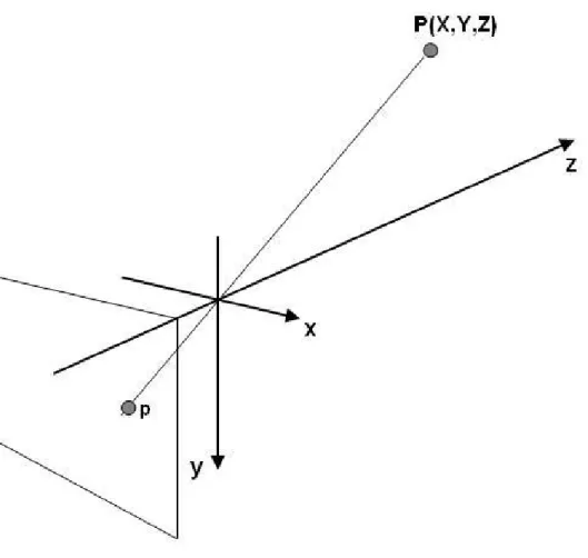
Pin-hole model

Classical geometric optics is based on models thick lens and thin lens. We start from the pin-hole model where all the rays passing through a single point, called

the optical center. The photosensitive cell (image plane) is at a distance f from the optical center, which is called focal length.

Figure 3 - Geometry of an imaging system

One can see that the image obtained is reversed with respect to the scene that the eye sees. To solve this problem lies in an artificial way the image plane in front of the optical center. From a physical point of view this is done by reading the CCD array so as to obtain a reverse image.

Perspective view projection

The perspective projection is a geometric abstraction in which the projection of a point is given by the cross of the visual image plane with the visual line that joins the point and the camera optical center.

From now on we will use the following notations: • Rc: the camera reference

• Rw: reference related to the modeling of object • (u, v): reference in the image

Figure 4 - Image plane in front of the optical center

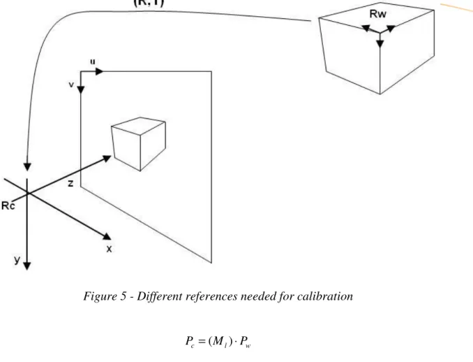
Reference change Object/Camera

The first change of reference allows to express the coordinates of the calibration (position in space) referenced to the camera, with a rotation and a translation.

Figure 5 - Different references needed for calibration w l c M P P =_{( )}⋅             =                   = 1 1 1 0 _c c c w w w c Z Y X Z Y X T R P

Pw are the 3D coordinates of a pattern point expressed in the model reference and Pc are the coordinates of the same point expressed in the camera reference

The rotation and translation matrices R3x3 and T3x1 are defined under the

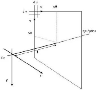
reference system of the camera Reference change Camera/Image

The change of reference to the image the camera is linked to the perspective projection equations. In classic mode these equations are expressed as follows

f z Z f Y y Z f X x c c c c = = = / /

In homogeneous coordinates the system is as follows: c P f f s sy sx           =           0 0 0 1 0 0 0 0 0 0

The homogeneous notation s introduces a multiplicative factor in the transformation R3, R2      = = = c c c Z s fY sy fX sx and substituting s:    = = c c c c Z fY y Z fX x / /

Change of coordinates to the image plane

It is about expressing x and y coordinates on the form of an elementary pixel CCD array. In particular, the digitization is a change of units (from mm to pixels) and a translation (of the reference of the camera to the beginning of the image plane at upper left corner)

                    =           s sy sx v dy u dx s sv su 1 0 0 / 1 0 0 / 1 0 0

Solving we have the classic reference exchange equations (coordinates of the camera / pixel coordinates):

   + = + = 0 0 / / v dy y v u dx x u

where (uo, vo) represent the coordinates (in pixels) in the image of the intersection of the optical axis and the image plane and (dx, dy) are the x and y dimensions of an elementary pixel array CCD camera

General expression

The whole system is expressed as follows:

                                              =           1 1 0 0 0 0 0 0 1 0 0 0 0 0 0 1 0 0 / 1 0 0 / 1 33 32 31 23 22 21 13 12 11 0 0 w w w z y x Z Y X T R R R T R R R T R R R f f v dy u dx s sv su

We have the next parameters:

• (Xw,Yw,Zw) are the coordinates 3D of pattern point

• (u,v) are the coordinates 2D of a pixel in the image of projected point • (uo,vo,f,dx,dy) are the intrinsic parameters of the calibration.

• R and T are the extrinsic parameters.

              =               =           1 1 ) 4 3 ( int w w x w w ext Z Y X M Z Y X M M s sv su w w

M is the matrix of calibration of the system is formed by five intrinsic parameters of the camera. Normally the matrix is expressed as

          = 0 0 0 1 0 / 0 0 0 / int ₀ 0 v u dy f dx f M Then: ) / / ( / / dx dy f f dy f f dx f f y x y x = →    = =

The relationship dx/dy represents the pixel relationship. Intrinsic parameters are 4, (fx, fy, uo, vo) in contrast, the extrinsic are 12, 9 for the rotation and 3 for the translation, which are independent of the camera

General formulation of the problem of calibration

Calibrating a vision system is to be able to determine all the parameters involved in the analytical expression of the formation of the image. The problem is formulated as follows, from a number of 3D-2D matches (Xw, Yw, Zw: u, v)

between a pattern and its image, determining the 16 parameters of image formation.

2.2

Calibration process using MATLAB

We will do the calibration process using the Matlab calibration toolbox. We start the GUI with the command calib_gui. The images processed are introduced

Figure 7 – Camera Calibration Toolbox GUI

The next step is to select the option of Extract grid corners. He asks us to introduce the size of the squares. We have to click as accurately as possible in four corners. The application automatically detects corners. This process is carried out with all the images. If the marked points do not correspond to the corners, we can introduce a distortion coefficient. The program will ask if we agree with the new result.

Figure 8 – Chessboard pattern images

Figure 9 – Extraction grid corners process

We select the option Show calib results, the parameters discussed above more distortion coefficients are shown.

Figure 10 – Camera parameters

This process must be done with the greatest precision possible, because these parameters will be of great importance. Together with the parameters we can

observe the error in pixel units. If this were large we would have to repeat the process until a smaller error.

Chapter 3

Feature extraction

A map is considered as set of point landmarks in the space. Therefore, feature extraction is the process that identifies landmarks in the environment. From an image, we must recognize and select the best points to be match because they will be tracked across multiple images. If the feature extraction were poor, this could lead to not converge to the filter.

There are several methods of extraction. Among them we can find three popular feature extractors used in visual SLAM: the Harris corner detector, the Kanade-Lucas-Tomasi tracker (KLT) and the Scale-Invariant Feature Transform (SIFT). In [7] is explained their differences and is done a qualitative study.

At first, we use the Harris detector but as in the end we use the implementation of Davison, the extraction was done manually. When we chose the first method, it was for its good results, its wide use, because it integrates well with the kalman filter. Also, because there are opencv functions already implemented.

3.1

The Harris Corner Detector

In general, when we use any corners detector, it is considered that a pixel is a corner when the derivative of the direction of the gradient exceeds a threshold at that point, and the magnitude of the gradient at that point also exceeds a threshold.

In the next expression of Harris detector, if H is low, the pixel will have more corner character.

This detector uses only first order derivative, Ix and Iy, <x> means convolution with a

Gaussian filter with a certain σ

3.2

Using OpenCV

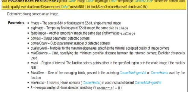
This is a function library specialized in image processing. It is available for C, C++ and Python. It has a large number of functions, among which we find cvGoodFeaturesToTrack. Through this function we extracted at first, the characteristics of the image. This function contains a number of parameters, they can specify the maximum number of corners we want to detect. We can

also specify the block size around each pixel where the function will perform the processing, the minimum distance between corners and other parameters shown in the next figure.

Figure 11 – Definition of function cvGoodFeaturesToTrack

Then we show the results of using the Harris detector using OpenCV library en Visual Studio

3.3

Davison’s application in MATLAB

As shown in the image below, the GUI has a button to manually select these features. Using previously the above function, we have a more precise idea of what points we need to select image. The GUI allows us to select the features in each frame. If any of these will not appear in the image, or have definitely been lost we may use this to add more.

Chapter 4

Data Association: Matching

After corner features are extracted the next step is to correctly match the features of the current image with as many features of the previous image as possible. As we said before, this is a very important and not trivial step. The kind of matching depends on the kind of features extraction and the framework. As we use corners as features instead of lines, edges or invariant descriptors and we work in Extended Kalman Filter (EKF) framework, the matching approach is a template matching via exhaustive correlation search. Measurement uncertainty regions derived from the filter constrain the search for matching features. There is an active search within elliptical search regions defined by the feature innovation covariance. All this will be explained in detail in the tracking section. Now we need to know that in these search regions the program calculates a cross-correlation to perform the matching.

Template matching is a technique in digital image processing for finding in general small parts of an image which match a template image. The basic method of template matching uses a convolution mask (template), tailored to a specific feature of the search image, which we want to detect.

4.1 Theorical explanation

The cross correlation in template matching is based on the Euclidean distance:

2 , , 2 )] , ( ) , ( [ ) , ( =

∑

(where f is the image and the sum is over x,y under the window containing the feature t positioned at u,v). In the expansion of d2

∑

∑

t is constant. If the term

∑

constant then the remaining cross-correlation term

∑

4.2 In the application

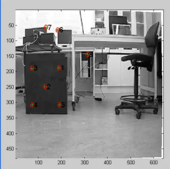
In the next figure we can watch in red color the search region . In the first steps the search regions are bigger because the uncertainty is also bigger.

Figure 14 – search regions in first steps

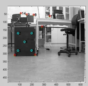
After some steps, the search regions are smaller:

Figure 15 – search regions after several steps

If we make a zoom we can watch with a red cross the matched point and with a red dot the predicted feature.

Figure 16 – predicted feature (red dot) and matched feature (green cross)

When there is a sudden movement this may produce not matching because the points were not in the search region. Then the points are shown in blue

Chapter 5

Tracking problem: Extended Kalman Filter (EKF)

This visual SLAM approach is located in an EKF Framework. The Kalman filter is an algorithm that predicts hidden states x, which cannot be measured in a dynamic process controlled by the following stochastic and linear difference equation, and by measures z.

The first equation is the model of the system and the second is the measurement model.

where:

wk is the process noise which is assumed to be drawn from a zero mean multivariate normal distribution with covariance Qk.

p(w) -> N(0,Q), Q = constant.

vk is the observation noise which is assumed to be zero mean Gaussian white noise with covariance Rk.

p(v) -> N(0,R), R = constant.

Kalman filter allows to identify the state xk from previous measurements uk, zk,

Qk, Rk and previous identifications of xk.

• F is the state transition matrix according to the state. • G is the control-input matrix based on the input u.

• H is the matrix that relates the state to the measure, the observation model.

Figure 18 – Prediction- Update

We do not actually use this filter, we use a similar one, the Extended Kalman Filter. This is a solution for nonlinear systems. This is linearized around the work point. In the first case the matrix are constant in all iterations, however in EKF we have function instead of matrix:

: update system function (camera motion) : measure system function

5.1 Motion model and state vector

Camera motion model

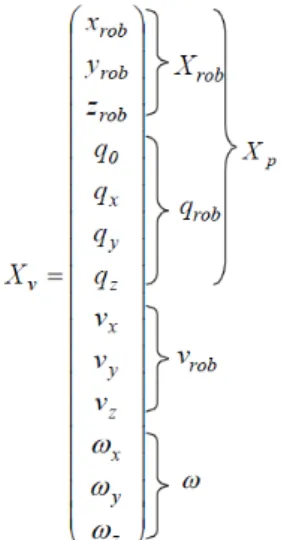
We assume a constant angular velocity and linear model to define the movement of the camera. The camera state xv is composed of:

The first three terms correspond to the absolute position of the robot, in our case, the camera, the following four with the quaternion defining the orientation of the camera on the global system, the next three with the linear velocity and the last three with the angular velocity

It is assumed that there are a linear and angular accelerations a and α. These affect the camera, producing at each step, an impulse of linear velocity V = a ∆t and angular velocity Ω = α∆t, with zero mean and known Gaussian distribution. A diagonal covariance matrix for the unknown input linear and angular accelerations are defined.

The state update equation for the camera is:

where q((ωkC +ΩC )∆t) is the quaternion defined by the rotation vector (ωkC +ΩC )∆t.

Euclidean XYZ Point Parametrization

Representation of the position of features in Euclidean coordinates is as follows:

.

Inverse Depth Point Parametrization

As we said in the introduction, the study of this research work has focused on a method developed by Javier Civera that encodes the position of the landmarks with 6 parameters instead of the three typical in Euclidean representation.

The yi vector encodes the ray from the first camera position from which the

feature was observed by xi, yi, zi , the camera optical center, and θi, φi azimuth

and elevation (coded in the world frame) defining unit directional vector m(θi,

Figure 19 – ray coded in I.D.P.

The next expression explains how to transform a 6-D point in 3-D:

Full state vector

As in other visual Slam approaches working in a EKF framework, we use a only sate vector. Therefore the full state vector is composed of xv and the 6D

5.2 Measurement model

Measurements related to the state by camera parameters and perspective projection. The measurement model predicts hi values based on:

• The absolute position of each landmark • The absolute position of the camera • The rotation matrix of the camera For points in Euclidean representation:

In Inverse depth parametrization:

With the next expression we transform the measurement to pixel units by the camera parameters

where u0 , v0 is the camera’s principal point, f is the focal length,

5.3 Prediction step

In this step the filter predicts the camera position and supposes that the features are in the same position. We have the full state vector and the covariance matrix:

Figure 20 – state vector and covariance matrix

Using the motion model we project the state ahead:

)

,

ˆ

(

ˆ

f

x

u

x

=

Figure 21 – prediction step, estimated position

The error covariance is projected ahead:

Q x f P x f P T new + ∂ ∂ ∂ ∂ =

Figure 22 – prediction step, error projection

5.4 Update step

First we measure features:

Figure 23 – update step, getting measurements

The innovation is calculated:

) ˆ (x h z − = ν

After calculating the innovation, we calculate the innovation covariance S and the Kalman Gain W:

1 − ∂ ∂ = + ∂ ∂ ∂ ∂ = S x h P W R x h P x h S T T

With the innovation and the Kalman Gain we update the estimate state and the error covariance: T new new WSW P P W x x − = + = ˆ

ν

In the next figure the uncertainty is smaller:

Chapter 6

Adjustments to our visual system & results

6.1 Video recording

At first, we started working with a webcam because the original idea was to test the algorithm in real time, in C. A small application was implemented to capture the webcam video in real time, extract the frames and remove the distortion of the frames. All this in Visual Studio using the OpenCV library. Then, we began using the platform of A.J.Davison, J.Civera and J.M.M. Montiel in MATLAB. In this environment the processing was not in real time because the frames were extracted and later worked with them. Anyway at first we were still using a webcam. This way we did not get sufficient quality videos, because there were many jumps, the video was not fluent. We did not get good results. Because of these leaps the matching failed. Because we were working with a camera motion model assumed an acceleration so bigger we could not get good results. Therefore we decided to work with a conventional camera, not a webcam. So we got videos more fluid, and consequently better results.

To verify the results, we recorded a video in the laboratory. This video consisted of a trajectory of a square with 50 cm of side.

6.2 Platform in MATLAB

The environment where this method has been proven Slam was MATLAB. The application consists of multiple files-M developed by different people, Andrew Davidson, Javier Civera, J.M.M. Montiel mainly. To run it we type:

>> mono_slam

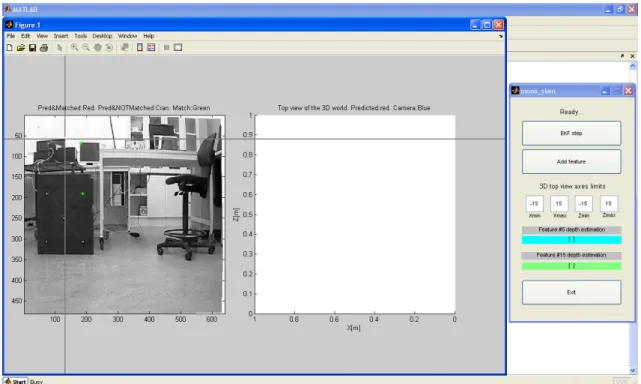
After that we can watch a figure with two graphs, on the left the frame that is set as initial and on the right a graph with the estimation of landmarks and surrounded by ellipses that indicate the uncertainty of the depth and the camera position in blue. The path traced by the camera appears in blue dots. As well as from the figure, a GUI is also shown with controls, a button to start the Kalman filter, other to add features, a control to modify the limits of the axes of the graph and finally indicators that show the Euclidean coordinates of marks 5 and 15.

Figure 25 – Davison’s GUI

6.3 Adjustments to our vision system

SetCamParameters

.

We start with the setCamParameters file in this file the parameters of the camera are configured. We changed the original data by the data obtained in the calibration. Introducing the focal length, distortion coefficients and the optical center.

SetParameteres

In this file we find most of the parameters except the camera set in the previous file. As well as the parameters that affect the graphs we can find parameters that affect the process of initialization.

• Step: default is 1, in this case we process all indexed images, if it were 2 we would read the half number of images. there would be more difference between one frame and another.

• Initial ρ: Actually it is not very important because if the filter works correctly the feature depths are corrected, but to ensure a good performance and as the most of the features were all very close to the camera, we changed to a value close to reality, 0.4, assuming an initial depth all the features of 2.5 m.

Mono_slam

This is the main file that opens the GUI, which loads the parameters, initializes the system and handles the callbacks for controls. Focusing on EKF filter, once we click the EKF button will produce the following: Load frame, prediction, prediction measures, matching and updating / correction of the filter.

In this file we have done several modifications:

• This parameter sets the time that takes from one frame to another, being used in the camera motion model and this predict the position of the camera. Originally this set to 1/30, since the video is 30 fps. When we did tests with this value, the distances drawn by the camera were much higher than reality. Therefore we had to reduce this parameter, in the end we assign to this parameter the value 1/90. Reducing the time increment between one frame and another, the search region calculated for the matching is less.

• Sigma_imageNoise: original value is 1 pixel. This parameter corresponds to the measurement noise. We modify up to 2, with this the filter has more uncertainty and the search region becomes larger. We have increased the value of this parameter and the next ones so that in the curves drawn the filter does not diverge and there was a correct matching.

• Sigma_aNoise: has a original value of 6 m/s² we changed to 8. • Sigma_alphaNoise: As in the previous case we changed to 8.

6.4 Results

In the following picture, we can see that at first the uncertainty is very high, so we see that the red ellipses are very elongated. Although the features positions are not exact yet, we can observe the features that are at the same distance are already are grouped in the graph e.g. the features in the black surface are separate of the rest.

Figure 26 – Results in first steps

In the next figure we zoom out

Figure 27 – Results in first steps alter zoom out

Figure 28 – The beginning of the first curve

As the number of iterations has increased, the uncertainty of the features is smaller.

We can watch the second segment is not so accurate, in the next chapter we will explain the reason

Figure39 – The end of the second segment.

For the correct operation of the filter, at least 14 features must be visible at all times. If we lose we need to add more. The feature 28 has been recently added, their uncertainty is greater than the others.

In the next image we see how is drawn the second curve.

Figure 32 – The end of the trajectory

The following image corresponds to the result of another simulation. In this case, we drew a full square with the same parameters, except that deltat is now worth 1/80. The form does not correspond with reality, but it gets close the loop and the distance of both the trajectory and the features are more accurate.

Although the plot by default is in 2D it is actually a representation in 3D, using the MATLAB tool indicated by an arrow you can rotate the view and watch the graph in 3D.

Figure 34 – Features in 3D

In the following picture we show a detail in 3D of the five point on the black surface. We can check the distribution and distance among them are correct.

Chapter 7

Conclusions and future works

7.1 Conclusions

After testing this visual approach Slam, we have realized the limitations of this type of application and improvements that can be performed.

In terms of features for the right performance, there must be at least 14 visible at all times and, ideally, they must be spread throughout the image.

We have also been aware of the limitations of not having odometry. These applications work much better in a robot that has odometry sensors. This would avoid using the model of camera movement.

Because of the fact that the camera is a bearing-only sensor. This means that the depth of a feature cannot be estimated from a single image measurement. The depth of the feature can be estimated only if the feature is observed from different points of view and only if the camera translates enough to produce significant parallax. In particular, it may take a very long time to obtain accurate estimates of the depths of distant features, since they display very little or no parallax when the camera moves small distances. (Parallax is an apparent displacement or difference in the apparent position of an object viewed along two different lines of sight, and is measured by the angle or semi-angle of inclination between those two lines).

Because of this we said before in the results section these were not so good. In order to get better results we should move the camera along of more distance. But application takes long time of processing between frames. In particular, to carry out the try showed in the last figure in results, it took one hour.

After this research work we have improved our knowledge about SLAM techniques and their different stages. We have checked the Kalman Filter performance being aware of its limitations.

7.2 Future work

A possible continuation of this work could be to implement this application in real time, in C language or other similar. For this we will have to use a web cam and change the manual extraction of features for an automatic extraction e.g. using Harris corners detector or other similar method.

After this implementation we could be test this application in a robot using odometry.

Chapter 8

References

[1] Inverse Depth Parametrization for Monocular SLAM Javier Civera, Andrew J. Davison, and J. M. Martínez Montiel

[2] A Visual Compass based on SLAM J. M. M. Montiel , Andrew J. Davison

[3] Modelling Stereoscopic Vision Systems for Robotic Applications Xavier Armangue Quintana

[4] Visual Odometry for Ground Vehicle

David Nistér, Oleg Naroditsky, James Bergen.

[5] Visual Odometry

David Nistér, Oleg Naroditsky, James Bergen. [6] Real Time Localization and 3D Reconstruction

E. Mouragnon , M. Lhuillier , M. Dhome , F. Dekeyser , P. Sayd.

[7] Quantitative Evaluation of Feature Extractors for Visual SLAM Jonathan Klippenstein, Hong Zhang

[8] Data Association in Stochastic Mapping using the Joint Compatibility Test José Neira, Juan D. Tardós

[9] Robust feature point extraction and Trucking for augmented reality Bruno Palacios Serra

[10] Visual 3-D SLAM from UAVs

Jorge Artieda, José M. Sebastian, Pascual Campoy, Juan F. Correa, Iván F. Mondragón Carol Martínez Miguel Olivares

[11] OpenCV Wiki

[12] Calibration of Stereoscopic systems: linear and photogrammetric approximation