DAGGTAX: A Taxonomy of Data Aggregation
Processes
Simin Cai, Barbara Gallina, Dag Nyström, and Cristina Seceleanu
Abstract—Data aggregation processes are essential constituents for data management in modern computer systems, such as
decision support systems and Internet of Things (IoT) systems. Due to the heterogeneity and real-time constraints in such systems, designing appropriate data aggregation processes often demands considerable efforts. A study on the characteristics of data aggregation processes will provide a comprehensive view for the designers, and facilitate potential tool support to ease the design process. In this paper, we propose a taxonomy called DAGGTAX, which is a feature diagram that models the common and variable characteristics of data aggregation processes, especially focusing on the real-time aspect. The taxonomy can serve as the foundation of a design tool that enables designers to build an aggregation process by selecting and composing desired features, and to reason about the feasibility of the design. We also provide a set of design heuristics that could help designers to decide the appropriate mechanisms for achieving the selected features. Our industrial case study demonstrates that DAGGTAX not only strengthens the understanding, but also facilitates the model-driven design of data aggregation processes.
Index Terms—data aggregation taxonomy, real-time data management, timeliness
F
1
I
NTRODUCTIONI
N modern information systems, data aggregation, defined as the process of producing a synthesized form from multiple data items [1], is commonly applied for data processing and management. For example, in order to discover unusual patterns and infer information, a data analysis application often computes a synthesized value from a subset of the database for statistical analysis [2]; in systems dealing with large amounts of data with limited storage, the data are often aggregated to save space [3]; in a sensor network, sensor data are aggregated, and only the aggregated data are transmitted so as to save bandwidth and energy [4]. Since data aggregation plays a key role in many applications, considerable research efforts have been dedicated to this topic. A number of taxonomies have been proposed to provide a comprehensive understanding on various aspects of data aggregation, such as aggregate functions ([1], [2], [5]), aggregation protocols ([4], [6], [7]) and security models ([8]).The focus of this paper is instead on another important aspect: the data aggregation process (or DAP for short) itself. We consider a DAP as three ordered activities that allow raw data to be transformed into aggregated data via an aggregate function. First, a DAP starts with preparing the raw data needed for the aggregation from the data source into the aggregation unit called the aggregator. Next, an aggregate function is applied by the aggregator on the raw data, and produces the aggregated data. Finally, the aggregated data may be further handled by the aggregator, for example, to be saved into storage or provided to other processes. The main constituents of these activities are the raw data, the aggregate function and the aggregated data.
The main contribution of this paper is a global, high-level characterization of data aggregation processes. We justify our study of the DAP by the fact that it represents a pillar of an
• S. Cai, B. Gallina, D. Nyström and C. Seceleanu are with the Mälardalen Real-Time Research Centre, Mälardalen University, Västerås, Sweden. Email: {simin.cai, barbara.gallina, dag.nystrom, cristina.seceleanu}@mdh.se
aggregation application’s workflow, no matter if it is a central-ized database management system or a highly distributed sensor network. Understanding DAP is essential to a correct design of the overall application. For instance, a sensor data gathering process, a data aggregation process and an analytic process form the basic workflow of a surveillance application. Multiple DAPs can also work together, one’s aggregated data being another’s raw data, to form a more complex, hierarchical aggregation process. To design a DAP, we must understand the desired features of its main constituents, that is, the raw data, the aggregate function and the aggregated data, as well as those of the DAP itself. Such features, ranging from functional features (such as data sharing) to extra-functional features (such as timeliness), are varying depending on different applications. One aspect of the understanding is to distinguish the mandatory features from the optional ones, so that the application designer is able to sort out the design priorities. Another aspect is to comprehend the implications of the features, and to reason about the (possible) impact on one another. Conflicts may arise among features, in that the existence of one feature may prohibit another one. Trade-offs should be taken into consideration at design time, so that infeasible designs can be ruled out at an early stage.
Among all features, we are particularly interested in the time-related properties of the DAP, since data aggregation is extensively applied in many real-time systems, such as automotive systems [9], avionic systems [10] and industrial automation [11]. In real-time systems, the correctness of a process depends on whether it completes on time, and validity of data depends on the time they are collected and accessed. These real-time properties are expected on raw data, aggregate function and the aggregated data, and impose constraints that cross-cut all three activities of a DAP. Therefore, we will especially emphasize the real-time related features and their implications.
In this paper we therefore propose a taxonomy of data aggre-gation processes, called DAGGTAX (Data AGGreaggre-gation TAXon-omy), with a focus on their features and consequent implications,
from the perspective of the aggregation process itself. The pro-posed taxonomy is presented as a feature diagram [12]. The aim of our taxonomy is to ease the design of aggregation processes, by providing a comprehensive view on the features and cross-cutting constraints, with a systematic representation. The latter can serve as the basis of a design tool, which enables selecting the desired features, reasoning about possible trade-offs, reducing the design space of the application, and composing the features to build the desired aggregation processes.
The remaining part of the paper is organized as follows. In Section 2 we discuss the existing taxonomies of data aggregation. In Section 3 we present the preliminaries, followed by a survey of data aggregation processes in scientific literatures in Section 4. Section 5 presents the proposed taxonomy, and in Section 6 we introduce the design rules and heuristics based on the implications of the features presented in the taxonomy. In Section 7 we validate the taxonomy by a case study from industry. Section 8 gives a further discussion of the implications of the real-time features, before concluding the paper in Section 9.
2
R
ELATEDW
ORKMany researchers have promoted the understanding of data ag-gregation on various aspects. Among these works, considerable efforts have been made on the study of aggregate functions. Mesiar et al. [13], Marichal [14], and Rudas et al. [1] have studied the mathematical properties of aggregate functions, such as continuity and stability, and discussed these properties of common aggregate functions in detail. A procedure for the construction of an ap-propriate aggregate function is also proposed by Rudas et al. [1]. In order to design a software system that computes aggregation efficiently, Gray et al. [2] have classified aggregate functions into distributive, algebraic and holistic, depending on the amount of intermediate states required for partial aggregates. Later, in order to study the influence of aggregate functions on the performance of sensor data aggregation, Madden et al. [5] have extended Gray’s taxonomy, and classified aggregate functions according to their state requirements, tolerance of loss, duplicate sensitivity, and monotonicity. Fasolo et al. [4] classify aggregate functions with respect to four dimensions, which are lossy aggregation, duplicate sensitivity, resilience to losses/failures and correlation awareness. Our taxonomy builds on these works that focus on the aggregate functions mainly, and provide a comprehensive view of the entire aggregate processes instead.
A large proportion of existing works have their focus on in-network data aggregation, which is commonly used in sensor networks. In-network aggregation is the process of processing and aggregating data at intermediate nodes when data are transmitted from sensor nodes to sinks through the network [4]. Besides a classification of aggregate functions that we have discussed in the previous paragraph, Fasolo et al. [4] classify the existing routing protocols according to the aggregation method, resilience to link failures, overhead to setup/maintain aggregation structure, scalability, resilience to node mobility, energy saving method and timing strategy. The aggregation protocols are also classified by Solis et al. [7], Makhloufi et al. [6], and Rajagopalan [15], with respect to different classification criteria. In contrast to the above works focusing mainly on aggregation protocols, Alzaid et al. [8] have proposed a taxonomy of secure aggregation schemes that classifies them into different models. All these works differ from our taxonomy in that they provide taxonomies from a different
perspective, such as network topology for instance. Instead, our work strives to understand the features and their implications of DAP and its constituents in design.
3
P
RELIMINARIESIn this section, we first recall the concepts of timeliness and temporal data consistency in real-time systems, after which we introduce feature models and feature diagrams that are used to present our taxonomy.
3.1 Timeliness and Temporal Data Consistency
In a real-time system, the correctness of a computation depends on both the logical correctness of the results, and the time at which the computation completes [16]. The property of completing the computation by a given deadline is referred to as timeliness. A real-time task can be classified as hard, firm or soft real-time, depending on the consequence of a deadline miss [16]. If a hard real-time task misses its deadline, the consequence will be catastrophic, e.g., loss of life or significant amounts of money. Therefore the timeliness of hard real-time tasks must always be guaranteed. For a firm real-time task, such as a task detecting vacant parking places, missing deadlines will render the results useless. For a soft real-time task, missing deadlines will reduce the value of the results. An example of soft real-time task is the signal processing task of a video meeting application, whose quality of service will degrade if the task misses its deadline.
Depending on the regularity of activation, real-time tasks can be classified as periodic, sporadic or aperiodic [16]. A periodic task is activated at a constant rate. The interval between two ac-tivations of a periodic task, called its period, remains unchanged. A sporadic task is activated with a Minimum INter-arrival Time (MINT), that is, the minimum interval between two consecutive activations. During the design of a real-time system, a sporadic task is often modeled as a periodic task with a period equal to the MINT. A sporadic task may also have a MAXimum inter-arrival Time (MAXT)which specifies the maximum interval between two consecutive activations. An aperiodic task is activated with an unpredictable interval between two consecutive activations. A task triggered by an external event with unknown occurrence pattern can be seen as aperiodic.
Real-time applications often monitor the state of the ment and react to changes accordingly and timely. The environ-ment state is represented as data in the system, which must be updated according to the actual environment state. The coherency between the value of the data in the system and its corresponding environment state is referred to as temporal data consistency, which includes two aspects, the absolute temporal validity and relative temporal validity[17]. A data instance is absolute valid, if the timespan between the time of sampling its corresponding real-world value, and the current time, is less than a specified absolute validity interval. A data instance derived from a set of data instances (base data) is absolute valid if all participating base data are absolute valid. A derived data instance is relative valid, if the base data are sampled within a specified interval, called relative validity interval.
Data instances that are not temporally consistent may lead to different consequences. Different levels of strictness with respect to temporal consistency thus exist, which are hard, firm and soft real-time, in a decreasing order of strictness. Using outdated hard real-time data could cause disastrous consequences, and therefore
Feature
(a) A mandatory feature
Feature (b) An optional feature
Feature1
Feature2
Feature3
(c) A group of alternative features
Feature [m..n]
(d) A feature with cardinality Fig. 1. Notations of a feature diagram
this should not appear. Firm real-time data are useless if they are outdated, whereas outdated soft real-time data can still be used, but will yield degraded usefulness.
3.2 Feature Model and Feature Diagram
The notion of feature was first introduced by Kang et al. in the Feature-Oriented Domain Analysis (FODA) method [12], in order to capture both the common characteristics of a family of systems as well as the differences between individual systems. Kang et al. define a feature as a prominent or distinctive system charac-teristic visible to end-users. Czarnecki and Eisenecker extend the definition of a feature to be any functional or extra-functional characteristic at the requirement, architecture, component, or any other level [18]. This definition allows us to model the char-acteristics of data aggregation processes as features. A feature model is a hierarchically organized set of features, representing all possible characteristics of a family of software products. A particular product can be formed by a combination of features, often called a configuration, selected from the feature model of its family.
A feature model is usually represented as a feature diagram [12], which is often depicted as a multilevel tree, whose nodes represent features and edges represent decomposition of features. In a feature diagram, a node with a solid dot represents a common feature (as shown in Fig. 1a), which is mandatory in every configuration. A node with a circle represents an optional feature (Fig. 1b), which may be selected by a particular configuration. Several nodes associated with a spanning curve represent a group of alternative features (Fig. 1c), from which one feature must be selected by a particular configuration. The cardinality [m..n] (n ≥ m ≥ 0) annotated with a node in Fig. 1d denotes how many instances of the feature, including the entire sub-tree, can be considered as children of the feature’s parent in a concrete configuration. If m≥1, a configuration must include at least one instance of the feature, e.g., a feature with [1..1] is then a manda-tory feature. If m=0, the feature is optional for a configuration.
A valid configuration is a combination of features that meets all specified constraints, which can be dependencies among fea-tures within the same model, or dependencies among different models. An example of such a constraint is that the selection of one feature requires the selection of another feature. Researchers in the software product line community have developed a number of tools, providing extensive support for feature modeling and the verification of constraints. For instance, in FeatureIDE [19], software designers can create feature diagrams using a rich graphic
interface. Designers can specify constraints across features as well as models, to ensure that only valid configurations are generated from the feature diagram.
4
A S
URVEY OFD
ATAA
GGREGATIONP
ROCESSESServing as an important information processing and analysis technique, data aggregation has been widely applied in a variety of information management systems. Based on scientific literature, in this section, we present a limited survey of application examples that implement data aggregation processes. In order to extract heuristics that help us generate our taxonomy, we select the exam-ples from a wide variety of application domains, and investigate the common and different characteristics of aggregation processes. Some of these examples are general-purpose infrastructures that implement aggregation as a basic service. The other examples develop data aggregation as ad hoc solutions suitable for the particular application scenarios.
In the following subsections, we first present how aggrega-tion is supported in different general-purpose infrastructures that provide data processing and management. Next, a number of ad hoc applications are presented, focusing on the requirements that the aggregation processes implemented in such applications must meet. Finally, we discuss the characteristics of aggregation processes exposed in the surveyed systems and applications.
4.1 General-purpose Infrastructures
In this subsection, we investigate the design of aggregation pro-cesses in general-purpose systems from the following domains: database management systems, data warehouses, data stream man-agement systems and wireless sensor networks.
Database Management Systems and Data Warehouses: Many information management systems adopt a general-purpose relational Database Management System (DBMS) or a Data Warehouse (DW) [20] as a back-end for centralized data man-agement, which have common aggregate functions implemented, and exposed as interfaces for users or programmers. Internally, aggregation is supported by a number of infrastructural services, including query evaluation, data storage and accessing, trigger mechanism, and transaction management. In a typical disk-based relational DBMS, as illustrated in Fig. 2, data are stored as tuples in the disk. An aggregation process is started by a query issued by a client. The DBMS then evaluates the query and loads the relevant tuples from disk into the main memory. An aggregate function is performed on the tuples and computes the aggregated value, which is then returned to the query issuer, cached in main memory or stored in the disk. An aggregation process can also be triggered by a state change in the database. Both raw data and aggregated data can be accessed by other processes. In order to maintain logical data consistency, such processes, including the aggregation process, are treated as transactions and governed by the transaction management system, which ensures the so-called ACID (Atomicity, Consistency, Isolation, and Durability) properties [21] during their executions.
Data can be aggregated by categories, usually specified in the "group-by" clause of a query. These categories may have a hierarchical relationship and thus represent the granularities of aggregation. For example, in a temporal database, users may choose to aggregate data by day, week or month, with a coarser granularity; in a spatial database, the aggregation can be based on streets, cities and provinces [22]. In a data warehouse, the stored
Disk DBMS Aggregate() request result Client reply query
Fig. 2. Illustration of aggregation in a disk-based DBMS
data usually have many dimensions, and the aggregation may need to be performed on multiple dimensions [20].
The aggregated value may be returned to the query issuer directly, or may be stored persistently in the database as a normal tuple. Alternatively, the aggregated values are cached in materialized views, so that other processes can make use of them [23]. It is common to store the aggregated values as materialized views in data warehouse since these results will be frequently used by analysis processes [20].
A number of aggregate functions are included in the SQL stan-dard and are commonly supported by general-purpose DBMSs. Other aggregate functions can be defined as user-defined func-tions. The aggregation can be triggered by an explicit query issued by the client, or by a trigger that reacts to the change of the database. In a data warehouse, aggregation is often planned periodically to refresh the materialized views using the updated base data. In case a query needs to access current data between the planned aggregation processes, extra aggregation processes may also be started to refresh the views [20].
Online Aggregation in Data Stream Management Sys-tems: Data aggregation in traditional DBMSs and DWs is per-formed like batch-processing: on a large number of tuples and in considerable time before returning the aggregated value. To im-prove performance and user experience, Hellerstein et al. propose “online aggregation” [24], which allows tuples to be aggregated incrementally. Tuples are selected from a base table by a sampling process, and aggregated with the cached partial aggregated result from previously sampled tuples. The partially aggregated value is available, which refers to the user as an approximate aggregated result. The aggregation process is defined with a stopping inter-face, through which the aggregation can be stopped, giving the approximate result as the final result.
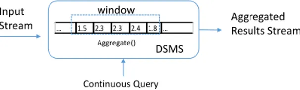
Online aggregation is often supported by Data Stream Man-agement Systems (DSMSs), which provide centralized aggrega-tion for continuous data streams. In Fig. 3, we illustrate the aggregation in a typical DSMS scenario. Usually, stream data are pushed into the DSMS continuously, often at a high frequency. Individual data instances are not significant, become stale as time passes, and do not need to be stored persistently. Finite subsets of the most recent incoming stream (“windows”) are cached in the system. Aggregate functions can be defined by users and are applied on the windows. In the Aurora data stream management system [25], the aggregate function can be associated with a “timeout” parameter, indicating the deadline of the computation of the function. A function should return before it times out, even if some raw data instances are missing or delayed, so as to provide timely response required by many real-time applications. Aurora has implemented a load shedding mechanism, which drops data instances when the system is overloaded. The aggregation is triggered either by continuous queries with specified periods, or by ad hoc queries which are issued by clients. The aggregated results are passed to the receiving application as an outgoing stream. To provide historical data, the aggregated data may also be kept
Continuous Query DSMS … 1.5 2.3 2.3 2.4 1.8 … window Aggregate() Input
Stream Aggregated Results Stream
Fig. 3. Illustration of aggregation in a data stream management system
n2 n1 n3 n4 n5 n6 Aggregate(n2, n3) Aggregate(n3, n4, n5, n6) sink Aggregate(n1, n2)
Fig. 4. Illustration of aggregation in a wireless sensor network
persistently for a specified period of time.
Multiple aggregation processes can be run concurrently, per-forming aggregation on the same data stream [26]. Oyamada et al. [27] point out that the aggregation in a DSMS may also involve non-streaming data, which can be shared and updated by other processes, causing potential data inconsistency. The authors propose a concurrency control mechanism to prevent the inconsistency.
In-network Aggregation in Wireless Sensor Networks: Data aggregation plays an essential role in Wireless Sensor Network (WSN) applications. In these applications, numerous data are gathered from resource-constrained sensor nodes that are deployed to monitor the environment. The gathered data are transmitted through a network to sink nodes, which are equipped with more resource for advanced computation and analysis. Along the transmission, data are aggregated in the intermediate sensor nodes or special aggregate nodes, in a decentralized topology. This aggregation technique is also called “in-network aggregation” [4]. In contrast, a sensor network can also apply centralized aggregation if the data of all sensors are transmitted to and aggregated in one single node. Fig. 4 gives an example of data aggregation in a sensor network. In this example, data from nodes n4, n5 and n6 are aggregated in node n3. This aggregated result is then transmitted to n2, and aggregated with the data of n2. Finally, the data from n2 and n1 are aggregated in the sink node.
Madden et.al [5] propose Tiny AGgregation (TAG), a generic aggregation service for ad hoc networks. In TAG, the user poses aggregation queries from a base station, which are distributed to the nodes in the network. Sensors collect data and route data back to the base station through a routing tree. As the data flow up the tree, it is aggregated by an aggregation function and value-based partitioning according to the query, level by level. At each level, a node awakens when it receives the aggregate request, together with a deadline when it should reply to its parent, and propagates the request to its children with an earlier deadline. Each node then listens to its children, aggregates the data transmitted from the children and the reading of itself, and then replies the aggregated result to its parent. If any node replies after its specified deadline, its value will not be aggregated by its parent, which means that the final aggregated result is actually an approximation.
Sensor-layer Aggregation
Sensor 1 Sensor 2 … Sensor N
Detection Confidence 1 Detection Confidence 2 Detection Confidence N … Node-layer Aggregation Group-layer Aggregation
Node 1 Node 2 … Node N
Group 1 … Group N Base-layer Aggregation
Fig. 5. Data Aggregation Architecture of VigilNet [29]
The aggregated results are cached by the nodes, and can be used for fault tolerance reason, e.g., loss of messages from a child. TAG has also classified aggregate functions into distributive, algebraic, holistic, unique and content-sensitive. Decentralized in-network aggregation is only appropriate for distributive and algebraic aggregate functions, since they can be decomposed into sub-aggregates. For other functions, all sensor data have to be collected to one node and aggregated together.
TAG is later implemented in the TinyDB [28], which supports SQL-style queries. Aggregation can be triggered periodically by continuous queries, or at once by a state change or an ad hoc query. Aggregated results can be stored persistently as storage points, which may be accessed by other processes.
4.2 Ad Hoc Applications
Many applications have unique requirements, and consequently use their ad hoc aggregation processes to fulfill their requirements. Examples of such applications are presented in the following paragraphs.
He et al. present the VigilNet for real-time surveillance with a tiered architecture [29]. Four layers are implemented in this system and each layer has its data aggregation requirements. The data aggregation architecture of VigilNet is illustrated in Fig. 5. The first layer is the sensor layer in which data inputs are pushed from individual sensors at specific rates, and aggregated as detection confidence vectors. In this layer the aggregation needs to meet stringent real-time constraints since the sensors send signals about fast-moving targets. The results of sensor-layer aggregation are sent to the node for node-layer aggregation. Each sensor node includes several sensors, and computes the average of sensor confi-dence vectors incrementally when a new sensor conficonfi-dence vector arrives. If the aggregated results show the existence of a tracking target, the node estimates the position of the target, and sends a report to the leading node of the local group. The leader buffers the reports from members, until the number reaches a predefined aggregation degree. Then, it aggregates all the reports, estimates the current position of the target, and sends the aggregated report to the base station. The base station aggregates the new report with historical positions of the target, and calculates the velocity using a linear regression procedure.
Defude et al. propose the VESPA (Vehicular Event Sharing with a mobile P2P Architecture) approach [30] for the Vehicular Ad hoc NETwork (VANET), to aggregate traffic information events, such as parking places, accidents and road obstacles, pushed from neighbor vehicles. The events are aggregated by times, areas and event types. The aggregated values are stored and accessed for further analysis.
Goud et al. [9] propose a real-time data repository for automo-tive adapautomo-tive cruise control systems. It includes an Environment Data Repository (EDR) and a Derived Data Repository (DDR). The EDR periodically reads sensor readings, aggregates them,
and keeps the aggregated value in the repository. The DDR then reads and aggregates the values from EDR, only when the changes of readings from some sensors exceed a threshold. The sensor data are real-time and have their validity intervals. The aggregate processes must complete before the data become invalid, and produce the results for other processes with stringent deadlines.
Arai et al. propose an adaptive two phase approach for ap-proximate ad hoc aggregation in unstructured peer-to-peer (P2P) systems [31]. When an ad hoc aggregate query is issued, in the first phase, sample peers are visited by a random walk from the sink, with a predefined depth. Information of the visited peers are collected to the sink, and analyzed to decide the peers to be aggregated. These peers are then visited in the second phase. For some aggregate functions such as COUNT and AVERAGE, partial aggregate results are computed in the local peer, and returned to the sink. For other aggregate functions, raw data are returned to the sink and aggregated in the sink.
Baulier et al. [32] propose a database system for real-time event aggregation in telecommunication systems. Events gener-ated by phone calls are pushed into the system, which should be aggregated within specific response times. The aggregated results are kept in a main-memory database as views for other time-critical processes. When a new event arrives, it triggers the aggregate process to update the aggregate view. The event record itself is stored into a data warehouse persistently, which is not time-critical.
Bar et al. [33] propose an online aggregation system for network traffic monitoring where large volumes of heterogeneous data streams are processed with different time constraints. Arriv-ing stream data instances, as well as non-stream data, are stored persistently in the system. Aggregation can be triggered by ad hoc queries, or triggered periodically by continuous queries. The aggregate results are stored persistently in materialized views. Aggregate functions are computed incrementally, by combining the newly arrived instance with cached aggregated results.
Bür et al. describe an online active control system for aircrafts which employs data aggregation [10]. In this application, real-time data are gathered periodically from sensors deployed in the aircraft, and aggregated periodically. Since the aircraft system is time-critical, the freshness of data and timely processing of aggregation are crucial.
Lee et al. propose an approach for aggregating data in an industrial manufacturing system [11]. Three types of aggregation are described, which are aggregation at device level, aggregation in control system, and aggregation in remote monitoring system. At device level, real-time raw data are produced by sensors and controllers, and are aggregated in the devices. The aggregation is triggered hourly, or by state changes in the device. The aggregation functions are simple calculations for hourly throughput, error count, etc. The aggregated values are sent to subscribing clients, namely the control system and the remote monitoring system. The control system receives the data from devices and store them into a database. Every hour, these data, together with other events, are aggregated to produce error times, throughput, etc. The remote monitoring system also stores the data from devices and performs aggregation. Delay could occur in aggregation in the remote system.
Iftikhar applies data aggregation on integration of data in farming systems [3]. Data are collected from different devices, and stored permanently in a relational database. A gradual granular data aggregation strategy is then applied on the stored data.
Basically, older data should be aggregated in a coarse-grained granularity while newer data are aggregated in a finer granularity. For different granularities, aggregation is triggered in different periods. The aggregated results are kept in the database while the raw data are deleted to save space.
Golab et al. propose a tool called DataDepot for generating data warehouses from streaming data feeds [34], focusing on the real-time quality of the data. Raw data are modeled as tables, which are not persistent and have a freshness property. Raw data are generated from different sources, with various properties such as rate and freshness. Raw tables are aggregated and stored in persistent derived tables which must also be fresh. Updates in the raw tables are propagated to the derived tables.
4.3 Survey Results
More than 13,000 research works are indexed in the SCOPUS search engine using “data aggregation” as a search key for title, abstract and keywords in computer science and engineering. Al-though only a small proportion of related works are examined here, our survey covers a relevant set of systems and application domains, which exposes the common and variable characteristics of the raw data, aggregated data, the aggregate functions, as well as the entire data aggregation processes.
In Table 1, we summarize the previous review by listing characteristics of the DAPs in the surveyed systems and appli-cations. Clearly, each aggregation process must have raw data, an aggregation function and the aggregated results. However, other characteristics have shown great variety. For instance, aggregation processes prepare the raw data ready for aggregation, by different data acquisition schemes. In some applications the aggregation process needs to pull the raw data from the persistent storage of the data source. Therefore the designer of an aggregation process must take this interaction into consideration. In other applications, however, raw data are pushed by the data source, so fetching raw data is not the concern of the aggregation process. The aggregated data may be stored persistently in some scenarios and are expected to survive system failures, while in other scenarios they can only reside in the volatile memory. As one can see in Table 1, the consistency of the data may depend on the time in some DAPs, while in others the data are static. A large variety of aggregate functions have been applied in aggregation processes, depending on the requirements of the particular application. The aggregation process itself may be scheduled periodically, or triggered by ad hoc events. In time-critical systems, the aggregation processes have strict timeliness requirements, while in some analytical systems with large amount of data the delays of the aggregation processes are tolerable. To design an appropriate aggregation process, it follows that one must take these characteristics, as well as their nature (necessity, optionality, etc) and their cross-cutting constraints, into consideration. A designer could benefit from having a systematic representation of these characteristics to ease the design, as well as support for facilitating feasible choices of the involved characteristics.
5
O
URP
ROPOSEDT
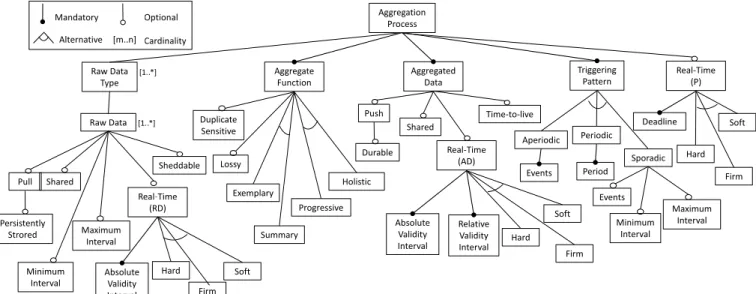
AXONOMYThe survey presented in Section 4 has revealed a number of characteristics of aggregation processes, including the raw data, the aggregated data, the aggregate functions, as well as the triggering patterns and the timeliness of the processes. Some of these characteristics are common for all aggregation processes,
while others are distinct from case to case. In this section we propose a taxonomy of data aggregation processes, as an ordered arrangement of features revealed by the survey. The taxonomy for these common and variable characteristics not only leads to a clear understanding of the aggregation process, but also lays a solid foundation for an eventual tool support for reasoning about the impact of different features on the design.
We choose feature diagram as the presentation of our tax-onomy, mainly due to two reasons. First, features may be used to model both functional and extra-functional characteristics of systems. This allows us to capture cross-cutting aspects that have on multiple software modules related to different concerns. Second, the notation of feature diagrams is simple to construct, powerful to capture the common and variable characteristics of different data aggregation processes, and intuitive to provide an organizational view of the processes. The taxonomy is shown in Fig. 6.
In the following subsections, these features are discussed in details with concrete examples. More precisely, the discussion is organized in order to reflect the logical separation of features. We explain Fig. 6 from the top level features under “Aggregation Process”, and iterate through all sub-features in a depth-first way. The top level features include “Raw Data”, “Aggregate Function” and “Aggregated Data”, which are the main constituents of an aggregation process. Features that characterize the entire DAP are also top level features, including the “Triggering Pattern” of the process, and “Real-Time (P)”, which refers to the timeliness of the entire process.
5.1 Raw Data
One of the mandatory features of real-time data aggregation is the raw data involved in the process. Raw data are the data provided by the DAP data sources. One DAP may involve one or more types of raw data. The multiplicity is reflected by the cardinality [1..*] next to the feature “Raw Data Type” in Fig. 6. Each raw data type may have a set of raw data. For instance, a surveillance system has two types of raw data (“sensor data” and “camera data”), while for the sensor data type there are several individual sensors with the same characteristics. Each raw data may have a set of properties, which are interpreted as its sub-features and constitute a sub-tree. These sub-features are: Pull, Shared, Sheddable, and Real-Time.
Pull: “Pull” is a data acquisition scheme for collecting raw data. Using this scheme, the aggregator actively acquires data from the data source, as illustrated in Fig. 7a. For instance, a traditional DBMS adopts the pull scheme, in which raw data are acquired from disks using SQL queries and aggregated in the main memory.
“Pull” is considered to be an optional feature of raw data, since not every DAP pulls data actively from data source. If raw data have the “pull” feature, pulling raw data actively from the data source is a necessary part of the aggregation process, including the selection of data as well as the shipment of data from the data source. If the raw data do not have the “pull” feature, they are pushed into the aggregator (Fig. 7b). In this case, in our view the action of pushing data is the responsibility of another process outside of the DAP. From DAP’s perspective, the raw data are already prepared for aggregation.
“Persistently Stored” is considered as an optional sub-feature of “Pull”, since raw data to be pulled from data source may be stored persistently in a non-volatile storage, such as a disk-based
TABLE 1
Characteristics of Data Aggregation Processes in the Surveyed Applications
Sample Raw Data Aggregate
Function
Aggregated Data Triggering Pattern Real-time Characteris-tics
relational disk-based DBMS/DW [20], [22], [23]
pulled from data sources; persis-tently stored; possibly shared by other processes
various functions
possibly durable; pos-sibly shared by other processes activated by events (queries or database triggers), or activated periodically usually no deadlines DSMS (AURORA [25], Oyamada et al. [27], Krishnamurthy et al. [26])
pushed by data sources; possibly pushed periodically; not persis-tently stored; cached for a par-ticular period; real-time; possibly shared by other processes; can be shedded
various functions
pushed to receiver; possibly durable; may be stored for a period of time
activated by events (ad hoc queries), or activated periodically (periodic continuous queries) deadlines depending on the application WSN (TAG [5], TinyDB [28])
pulled from data sources; not persistently stored; possibly be skipped
various functions
cached for a par-ticular period; pos-sibly durable; real-time; possibly shared by other processes activated by events, or activated periodically deadlines depending on the application VigilNet [29], sensor layer
pushed by data sources; not per-sistently stored; real-time; pushed periodically
detection confidence function
pushed to receiver; not durable
activated periodically hard deadlines
VigilNet [29], node layer
pushed by data sources; not per-sistently stored
average pushed to receiver; not durable
activated by event soft deadlines
VigilNet [29], group layer
pushed by data sources; cached for a particular period
ad hoc cal-culation
pushed to receiver; not durable
activated by event soft deadlines
VigilNet [29], base layer
pushed by data sources; persis-tently stored
regression shared by other pro-cesses
activated by event soft deadlines
VESPA [30] pushed by data sources various functions
durable; shared by other processes
activated by events soft deadlines
Goud et al. [9], EDR pulled from data sources; pulled periodically; real-time; not persis-tently stored
various functions
not durable; real-time; shared by other pro-cesses
activated periodically hard deadlines
Goud et al. [9], DDR pulled from data sources; real-time; not persistently stored
various functions
durable; real-time activated by events hard deadlines
Arai et al. [31] pulled from data sources; not per-sistently stored
various functions
possibly durable activated by events no deadlines
Baulier et al. [32] pushed by data sources; persis-tently stored
various functions
real-time; not durable; shared by other pro-cesses
activated by events hard deadlines
Bar et al. [33] pushed by data sources; persis-tently stored; possibly real-time
various functions
durable activated by events, or activated periodically
soft deadlines
Bür et al. [10] pushed by data sources; not per-sistently stored; real-time;
various functions
not durable; real-time activated periodically hard deadlines
Lee et al. [11], device level
pushed by data sources; real-time various functions
pushed to receiver; not durable
activated by events, or activated periodically
soft deadlines
Lee et al. [11], control system
pulled from data sources; persis-tently stored
various functions
possibly durable activated periodically soft deadlines
Lee et al. [11], remote monitoring system
pulled from data sources; persis-tently stored
various functions
possibly durable activated periodically soft deadlines
Iftikhar [3] pulled from data sources; persis-tently stored; stored for a partic-ular period; possibly shared by other processes
various functions
durable; stored for a particular period; pos-sibly shared by other processes
activated periodically soft deadlines
DataDepot [34] pulled from data sources; not per-sistently stored; possibly shared by other processes; real-time
various functions
durable; real-time activated by events deadlines depending on the application
Aggregation Process Raw Data Aggregate Function Pull Shared Real-Time (RD) [1..*] Persistently Strored Sheddable Minimum Interval Hard Firm Soft Duplicate Sensitive Exemplary Summary Progressive Holistic Triggering Pattern Aperiodic Periodic Aggregated Data Push Shared Real-Time (AD) Durable Hard Firm Soft Absolute Validity Interval Relative Validity Interval Real-Time (P) Deadline Hard Firm Soft Time-to-live Period Absolute Validity Interval Lossy [m..n] Mandatory Optional Alternative Cardinality Raw Data Type [1..*] Sporadic Events Events Minimum Interval Maximum Interval Maximum Interval
Fig. 6. The taxonomy of data aggregation processes
Data
Source 2. raw data Aggregator 1. request
(a) Pull scheme
Data
Source Aggregator
raw data
(b) Push scheme Fig. 7. Raw data acqusition schemes
relational DBMS. The retrieval of persistent raw data involves locating the data in the storage and the necessary I/O.
Shared: Raw data of some DAP examples in Section 4 are read or updated by other processes at the same time when they are read for aggregation [3], [26], [27]. The same raw data may be aggregated by several DAPs, or accessed by processes that do not perform aggregations. We use the optional “shared” feature to represent the characteristic that the raw data involved in the aggregation may be shared by other processes in the system.
Sheddable: We classify the raw data as “sheddable”, which is an optional feature, used in cases when data can be skipped for the aggregation. For instance, in TAG [5], the inputs from sensors will be ignored by the aggregation process if the data arrive too late. In a stream processing system, new arrivals may be discarded when the system is overloaded [25]. For raw data without the sheddable feature, every instance of the raw data is crucial and has to be computed for aggregation.
Real-Time (RD): The raw data involved in some of the surveyed DAPs have real-time constraints. Each data instance is associated with an arrival time, and is only valid if the elapsed time from its arrival time is less than its absolute validity interval. “Real-time” is therefore considered an optional feature of raw data, and “absolute validity interval” is a mandatory sub-feature of the “real-time” feature. We name the real-time feature of raw data as “Real-Time (RD)” in our taxonomy, for differentiating from the real-time features of the aggregated data (“Real-Time (AD)” in Section 5.3) and the process (“Real-Time (P)” in Section 5.5).
Raw data with real-time constraints are classified as “hard”,
“firm” or “soft” real-time, depending on the strictness with respect to temporal consistency. They are represented as alternative sub-features of the real-time feature. As we have explained in Section 3, hard real-time data (such as sensor data from a field device [11]) and firm real-time data (such as surveillance data [29]) must be guaranteed up-to-date, while outdated soft real-time data are still of some value and thus can be used (e.g., the derived data from a neighboring node in VigilNet [29]).
MINT: Raw data may arrive continuously with a Mini-mum INter-arrival Time (MINT), of which a fixed arrival time is a special case. For instance, in the surveillance system VigilNet [29], a magnetometer sensor monitors the environment and pushes the latest data to the aggregator at a frequency of 32HZ, implying a MINT of 32.15 milliseconds. We consider “MINT” an optional feature of the raw data.
5.2 Aggregate Function
An aggregation process must have an aggregate function to com-pute the aggregated result from raw data. An aggregate function exhibits a set of characteristics that we interpret as features.
Duplicate Sensitive: “Duplicate sensitivity” has been introduced as a dimension by Madden et al. [5] and Fasolo et al. [4]. An aggregate function is duplicate sensitive, if an incorrect aggregated result is produced due to a duplicated raw data. For example, COUNT, which counts the number of raw data instances, is duplicate sensitive, since a duplicated instance will lead to a result one bigger than it should be. MIN, which returns the minimum value of a set of instances, is not duplicate sensitive because its result is not affected by a duplicated instance. “Duplicate sensitive” is considered as an optional feature of the aggregate function.
Exemplary or Summary: According to Madden et.al [5], an aggregate function is either “exemplary” or “summary”, which are represented as alternative features in our taxonomy. An exemplary aggregate function returns one or several representative values of the selected raw data, for instance, MIN, which returns the minimum as a representative value of a set of values. A sum-mary aggregate function computes a result based on all selected
raw data, for instance, COUNT, which computes the cardinality of a set of values .
Lossy: An aggregate function is “lossy”, if the raw data cannot be reconstructed from the aggregated data alone [4]. For example, SUM, which computes the summation of a set of raw data instances, is a lossy function, as one cannot reproduce the raw data instances from the aggregated summation value without any additional information. On the contrary, a function that concatenates raw data instances with a known delimiter is not lossy, since the raw data can be reconstructed by splitting the concatenation. Therefore, we introduce “lossy” as an optional feature of aggregate functions.
Holistic or Progressive: Depending on whether the com-putation of aggregation can be decomposed into sub-aggregations, an aggregate function can be classified as either “progressive” or “holistic”. The computation of a progressive aggregate func-tion can be decomposed into the computafunc-tion of sub-aggregates. In order to compute the AVERAGE of ten data instances, for example, one can compute the AVERAGE values of the first five instances and the second five instances respectively, and then compute the AVERAGE of the whole set using these two values. The computation of a holistic aggregate function cannot be decomposed into sub-aggregations. An example of holistic aggregate function is MEDIAN, which finds the middle value from a sequence of sorted values. The correct MEDIAN value cannot be composed by, for example, the MEDIAN of the first half of the sequence together with the MEDIAN of the second half.
5.3 Aggregated Data
An aggregation process must produce one aggregated result, denoted as mandatory feature “Aggregate Data” in the feature diagram. Aggregated data may have a set of features, which are explained as follows.
Push: In some survey DAP examples, sending aggregated data to another unit of the system is an activity of the aggre-gator immediately after the computation of aggregation. This is considered as an active step of the aggregation process, and is represented by the feature “push”. For example, in the group layer aggregation of VigilNet [29], each node sends the aggregated data to its leading node actively. An aggregation process without the “push” feature leaves the aggregate results in the main memory, and it is other processes’ responsibility to fetch the results.
The aggregated data may be “pushed” into permanent storage, such as in [32] and [11]. The stored aggregated data may be required to be durable, which means that the aggregated data must survive potential system failures. Therefore, “durable” is considered as an optional sub-feature of the “push” feature.
Shared: Similar to raw data, the aggregated data has an optional “shared” feature too, to represent the characteristic of some of the surveyed DAPs that the aggregated data may be shared by other concurrent processes in the system. For instance, the aggregated results of one process may serve as the raw data inputs of another aggregation process, creating a hierarchy of aggregation [25], [29]. The results of aggregation may also be accessed by a non-aggregation process, such as a control process [9].
Time-to-live: The “time-to-live” feature regulates how long the aggregated data should be preserved in the aggregator. For instance, Aurora system [25] can be configured to guarantee that the aggregated data are available for other processes, such as an archiving process or another aggregate process, for a certain
period of time. After this period, these data can be discarded or overwritten. We use the optional feature “time-to-live” to represent this characteristic.
Real-Time (AD): The aggregated data may be real-time, as required in some of the surveyed DAPs, if the validity of the data instance depends on whether its temporal consistency constraints are met. Therefore the “real-time” feature, which is named “Real-Time (AD)”, is an optional feature of aggregated data in our taxonomy. The temporal consistency constraints on real-time aggregated data include two aspects, the absolute validity and relative validity, as explained in Section 3. “Absolute validity interval” and “relative validity interval” are two mandatory sub-features of the “Real-Time (AD)” feature.
Similar to raw data, the real-time feature of aggregated data has “hard”, “firm” and “soft” as alternative sub-features. If the aggregated data are required to be hard real-time, they have to be ensured temporal consistent in order to avoid catastrophic consequences [32]. Compared with hard time data, firm real-time aggregated data are useless if they are not temporal consistent [29], while soft real-time aggregated data can still be used with less value (e.g., the aggregation in the remote server [11]).
5.4 Triggering Pattern
“Triggering pattern” refers to how the DAP is activated, which is a mandatory feature. We consider three types of triggering patterns for the activation of DAPs, represented by the alternative sub-features “periodic”, “sporadic” and “aperiodic”.
A periodic DAP is invoked according to a time schedule with a specified “Period”. A sporadic DAP could be triggered by an external “event”, or according to a time schedule, possibly with a “MinT” (Minimum inter-arrival Time) and/or “MaxT” (Maximum inter-arrival Time). An aperiodic DAP is activated by an external “event” without a constant period, MinT or MaxT. The event can be an aggregate command (e.g. an explicit aggregation query [28]) or a state change in the system [32].
5.5 Real-time (P)
Real-time applications, such as automotive systems [9] and in-dustrial monitoring systems [11], require the data aggregation process to complete its work by a specified deadline. The process timeliness, named “Real-Time (P)”, is considered as an optional feature of the DAP, and “deadline” is its mandatory sub-feature.
Aggregation processes may have different types of timeliness constraints, depending on the consequences of missing their dead-lines. For a soft real-time DAP, a deadline miss will lead to a less valuable aggregated result [30]. For a firm real-time DAP [11], the aggregated result becomes useless if the deadline is missed. If a hard real-time DAP misses its deadline, the aggregated result is not only useless, but hazardous [9], [10]. “Hard”, “firm” and “soft” are alternative sub-features of the timeliness feature.
We must emphasize the difference between timeliness (“Real-Time (P)”) and real-time features of data (“Real-(“Real-Time (RD)” and “Real-Time (AD)”), although both of them appear to be classified into hard, firm and soft real-time. Timeliness is a feature of the aggregation process, with respect to meeting its deadline. It specifies when the process must produce the aggregated data and release the system resources for other processes. As for real-time features of data, the validity intervals specify when the data become outdated, while the level of strictness with respect to temporal consistency decides whether outdated data could be used.
To meet the desired real-time strictness level of the data, the DAP may need to meet certain timeliness requirements, which will be discussed further in Section 6.
6
D
ESIGNR
ULES ANDH
EURISTICSIn the previous section we have introduced our taxonomy that encompasses the important features of a DAP. In this section, we formulate a set of design rules and heuristics, following the design implications imposed by the features. The design rules are the axioms that should be applied during the design. Violating the rules will result in infeasible feature combinations. Design heuristics, on the other hand, suggest that certain mechanisms may be needed, either to implement the selected features, or to mitigate the impact of the selected features.
6.1 Design Rules
The real-time features of data and process are commonly desired features of DAPs among real-time applications. Among these features there exist dependencies, which should be respected when one is selecting and combining these features. In this subsection we analyze the dependencies among the real-time data features (the “Real-Time (RD)” and “Real-Time (AD)” features in the tax-onomy) and the timeliness feature (the “Real-Time (P)” feature) of the aggregation process itself. Based on the analysis we formulate three design rules to eliminate the infeasible combinations.
As already introduced, real-time data can be classified as hard, firm or soft real-time according to the strictness w.r.t. the temporal consistency. The hard real-time feature imposes strongest constraints and represents highest level of strictness, while the soft real-time feature represents the lowest level of strictness. From the raw data to the aggregated data, the level of strictness can only decrease or remain the same. This is because the validity of aggregated data depends on the validity of raw data. Since the hard real-time aggregated data have to be both absolute valid and relative valid, which requires all involved raw data to be absolute valid, the raw data have to be hard real-time too. If the raw data is soft real-time, which indicates that outdated raw data may occur, the temporal consistency of the aggregated data cannot be guaranteed. Therefore, we get the following rule:
Rule 1: The real-time strictness level of the raw data must be higher than or equal to the real-time strictness level of the aggregated data.
The timeliness of the entire data aggregation process has an impact on meeting the strictness level of the aggregated data, since the validity of the aggregated data depends on the interval between the time when raw data are collected, and the time when the aggregated data are produced. If the aggregated data are required to be hard real-time, the DAP also has to be hard real-time. If the timeliness of the DAP is soft, the calculation may miss its deadline and produce an outdated aggregated result. If we consider the “hard”, “firm” and “soft” features of the DAP as levels of strictness w.r.t. timeliness, this rule is formulated as follows:
Rule 2: The strictness level w.r.t. timeliness of the entire DAP must be higher than or equal to the real-time strictness level of the aggregated data.
The fact that both the raw and aggregated data may be shared by multiple processes imposes further consideration on the real-time strictness of the shared data. If the raw data or the aggregated data are shared by several processes, and the requirements of these processes impose different real-time strictness, then the real-time
constraint of this data is in accordance with the highest strictness required by these processes. For example, the raw data of an aggregate process happens to be the input of a control process that demands the input to be hard real-time. Even though the aggregation process can tolerate outdated raw data, the real-time strictness level of the data must be hard. Otherwise the data for the control process may be outdated and lead to catastrophic consequences. Hence we formulate the following rule:
Rule 3: The real-time strictness of the raw/aggregated data must meet the highest real-time strictness level imposed by all processes that share the data.
These rules should be applied when the application designer analyzes the features derived from the requirement specification. Consider a process aggregating data from three sensors and pro-viding its aggregated data to a hard real-time control process. The specification of the aggregation process may allow outdated raw data, i.e., soft real-time raw data, and tolerate occasional deadline miss. However, since the control process requires its inputs (the aggregated data) to be hard real-time, both the raw data from the sensors and the DAP have to be hard real-time as well.
6.2 Design Heuristics
Accomplishing the design of a DAP involves the design of appro-priate supporting run-time mechanisms. These mechanisms either achieve the selected features of the DAP, or mitigate the impact of the selected features in order to ensure other properties of the system. Such properties could be, for instance, the logical data consistency characterized by the ACID properties of the processes. In this subsection we introduce a set of design heuristics, which are suggestions of mechanisms that could be implemented in order to enforce certain features and system properties. The heuristics are organized as suggested mechanisms as follows.
Synchronization for “pull” and “push” features: Pulling raw data from a data source may involve locating the data source, selecting the data and shipping data into the aggregator. Pushing aggregated data may involve locating the receiver and transmitting the data. These activities introduce higher risks of delayed and missing data that may breach the temporal and logical data consistency. Overheads in time and computation resource are also introduced, which are impacting factors of the overall timeliness of the process. When designing for such systems, one may consider developing a synchronization protocol to mitigate such impacts and ensure the consistency of the data.
Load shedding for “sheddable” feature combined with real-time features: Situations could occur when the DAP is not able to meet the real-time constraints, due to, for example, system overload. If the raw data are sheddable, one may consider implementing the load shedding mechanism [25], which allows raw data instances to be discarded systematically.
Approximation for “sheddable” feature combined with real-time features: An alternative mechanism for sheddable raw data is to implement approximation techniques. For example, Deshpande et al. introduce an approximation technique into sensor network to improve the efficiency of aggregation [35]. Instead of reading data from all sensors, the DAP only collects raw data from some of the sensors that fulfill a probabilistic model.
Concurrency control for “shared” feature: An impli-cation of shared data is the concern of logical data consistency, which is a common consideration from concurrent data access. A certain form of concurrency control needs to be implemented to
achieve a desired level of consistency. For example, the aggregate process may achieve full isolation from other processes, i.e., they can only see the aggregated result when the DAP completes, using serializable concurrency control [36]. To improve performance or timeliness, one may choose a less stringent concurrency control that allows other processes to access the sub-aggregate results of the DAP, which may lead to a less accurate final result. Without any concurrency control, the aggregation process may produce incorrect results using inconsistent data [37].
Logging and recovery for “durable” feature: In order to ensure the “durable” aggregated data, logging and backward failure recovery techniques, which are commonly used to achieve durability in data management systems, may be applied to the DAP. For example, the operations on the aggregated data are logged immediately, and the actual changes are written into the storage periodically.
Filtering for “duplicate sensitive” aggregate functions: Using a duplicate sensitive aggregate function indicates a higher risk of inconsistency caused by duplicated values sent to aggre-gator. A filtering mechanism may be implemented to identify the duplicates and filter them away.
Caching for “lossy” aggregate functions: Lossy aggre-gate functions disallow the reconstruction of raw data from the aggregated data. However, raw data may be needed to redo all changes when errors occur, in order to ensure the atomicity of a process. A caching mechanism may be implemented for the DAP as a solution, that raw data instances are cached in the aggregator until the process completes.
Decomposition of aggregation for “progressive” aggre-gate functions: The implication of using a progressive aggreaggre-gate function is that one may decompose the entire aggregation into sub-aggregates. Computing the sub-aggregates in parallel may benefit the performance of the entire DAP. Another useful applica-tion of the decomposiapplica-tion is error handling, especially when it is combined with a caching mechanism. Consider an aggregate pro-cess fetching data from several sensors. The propro-cess can perform aggregation upon the arrival of each sensor data and cache the sub-aggregate result so far. If an error occurs during the fetching of next sensor, the process can return the cached sub-aggregate result as an approximation [5], or only restart the fetching of the failed sensor, instead of restarting the whole process.
Buffers for raw data and aggregated data: Raw data ar-rive in the aggregator with their “MINT”, which could be different from the aggregation interval imposed by the“triggering pattern” of the process. Buffers may be necessary to keep the raw data available for aggregation. Buffers may also be necessary for the aggregated data, since the aggregated data are generated according to the “triggering pattern”, and must be available for a specified period defined by the “time-to-live” feature. Buffer management is crucial for the accuracy of aggregation as well as the resource utilization. For instance, circular buffer is a common mechanism in embedded systems for keeping data in limited memory. When the buffer is full, the program will just overwrite the old content with new data from the beginning. With the features presented in our taxonomy, one may calculate buffer size based on worst-case scenarios for non sheddable data, or suffice buffer size for sheddable data, given the size of each data instance.
Program Trace Macrocell (PTM) PTM Cluster Buffer
System Trace Macrocell (STM) STM Cluster Buffer
Software Instrumentation Dedicated System Memory
Hardware 1 Hardware n Debugger Function
Fig. 8. General architecture of the Hardware Assisted Trace system
7
E
VALUATION:
ANI
NDUSTRIALC
ASES
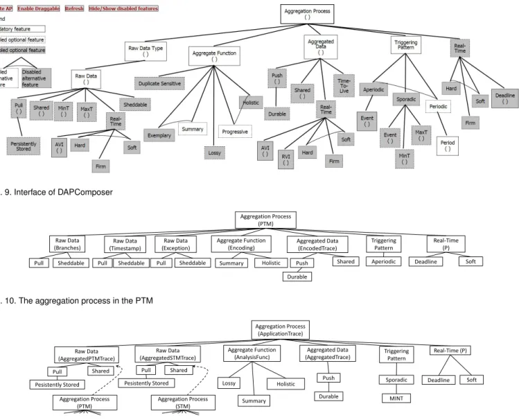
TUDYIn this section we evaluate the usefulness of our taxonomy in the design of a data aggregation application. Prior to the case study we have implemented a tool called DAPComposer (Data Aggregation Process Composer), shown in Fig. 9. The tool provides a graphical user interface for designers to create DAPs, by selecting and arranging the features in the diagram. Rules of mandatory, optional and alternative features are implemented. The mandatory features are always enabled, while optional and alternative features can be enabled/disabled by double-clicking the features. Annotations can be added to the selected features, such as the name of the data, or the actual value of the timing properties. It can also hide disabled features to provide a cleaner representation. Constraints can be typed as rules by users and saved in a rule base. The tool then validates the design against the specified rules. Although to the date only primitive constraints intrinsic to the feature model are checked by DAPComposer, we plan to mature the tool with more sophistic analysis capabilities, such as timing analysis, in the next version.
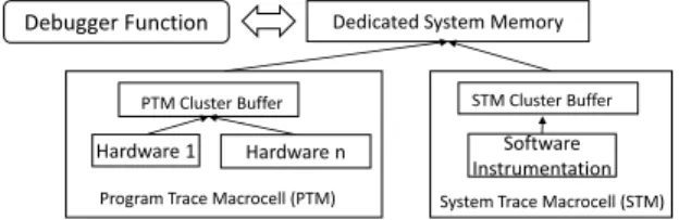
This evaluation is conducted on an industrial project, the Hardware Assisted Trace (HAT) [38] framework, together with its proposers from Ericsson. HAT, as shown in Fig. 8, is a framework for debugging functional errors in an embedded system. In this framework, a debugger function runs in the same system as the debugged program, and collects both hardware and software run-time traces continuously. Together with the engineers we have analyzed the aggregation processes in their current design. At a lower level, a Program Trace Macrocell (PTM) aggregation process aggregates traces from hardware. These aggregated PTM traces, together with software instrumentation traces from the Sys-tem Trace Macrocell (STM), are then aggregated by a higher level ApplicationTrace aggregation process, to create an informative trace for the debugged application.
We have analyzed the features of the PTM aggregation process and the ApplicationTrace aggregation process in HAT based on our taxonomy. The features of the PTM aggregation process are presented in Fig. 10. Triggered by computing events, this process pulls raw data from the local buffer of the hardware, and aggregates them using an encoding function to form an aggregated trace into the PTM cluster buffer. The raw data are considered sheddable, since they are generated frequently, and each aggregation pulls only the data in the local buffer at the time of the triggering event. The aggregated PTM and STM traces then serve as part of the raw data of the ApplicationTrace aggregation process, which is shown in Fig. 11. The ApplicationTrace process is triggered sporadically with a minimum inter-arrival time, and aggregates its raw data using an analytical function. The raw data of the ApplicationTrace should not be sheddable so that all aggregated traces are captured.
Fig. 9. Interface of DAPComposer Aggregation Process (PTM) Raw Data (Branches) Aggregate Function (Encoding) Summary Holistic Triggering Pattern Aperiodic Aggregated Data (EncodedTrace) Push Shared Real-Time (P) Deadline Soft Raw Data (Timestamp) Pull Raw Data (Exception) Pull Pull Durable Sheddable Sheddable Sheddable
Fig. 10. The aggregation process in the PTM
Aggregation Process (ApplicationTrace) Raw Data (AggregatedPTMTrace) Aggregate Function (AnalysisFunc) Summary Holistic Triggering Pattern Sporadic Aggregated Data (AggregatedTrace) Push Real-Time (P) Deadline Soft Lossy Raw Data (AggregatedSTMTrace) Pull Pull Durable Pesistently Stored Shared Pesistently Stored Shared Aggregation Process (PTM) MINT Aggregation Process (STM)
Fig. 11. The aggregation processes in the investigated HAT system
7.1 Problem identified in the HAT design
With the diagrams showing the features of the aggregation pro-cesses, the engineers could immediately identify a problem in the PTM buffer management. In the current design, the buffer size is decided by both the hardware platform and the designer’s experiences. The problem is that, the data in the buffer may be overwritten before they are aggregated. This problem has been observed on Ericsson’s implemented system, and awaits a solution. However, if the taxonomy would have been applied on the system design, this problem could have been identified before it was propagated to implementation.
This problem arises due to the lack of a holistic consideration on the PTM aggregation process and the ApplicationTrace ag-gregation process at design time. Triggered by aperiodic external events, the PTM process could produce a large number of traces within a short period and fill up the PTM buffer. The Applica-tionTrace process, on the other hand, is triggered with a minimum inter-arrival time, and consumes the PTM traces as unsheddable raw data. When the inter-arrival time of the PTM triggering events is shorter than the MINT of the ApplicationTrace process, the PTM traces in the buffer may be overwritten before they could be aggregated by the ApplicationTrace process.
7.2 Solutions
Providing a larger buffer could be a choice to mitigate this problem. However, a larger provision might either still fail to meet the buffer consumption in some rare cases, or become a loss of resource due to pessimism. Considering the resource-constrained nature of the system, a better way is to derive the necessary buffer size at design time, given the size of each data entry. Based on our taxonomy, we and Ericsson engineers have come up with two alternative design solutions to fix this problem. Both solutions reuse most of the features in the current design.
Solution 1: To be able to derive the worst-case buffer size, one solution is to ensure more predictable behaviors of the aggregation processes, by adjusting the following features in the diagram (see Fig. 12a): (i) Instead of selecting the “aperiodic” feature, the PTM process should select “sporadic”, with a defined MINT; and, (ii) the “sporadic” feature of the ApplicationTrace process should be replaced by “periodic”, so that the frequency of consuming the aggregated PTM traces can be determined. These changes of the features entail introducing extra real-time mechanisms into the current design, such as an admission control to ensure the MINT and a scheduler to schedule the processes. In addition, a “time-to-live” feature, whose value equals to the period
![Fig. 5. Data Aggregation Architecture of VigilNet [29]](https://thumb-eu.123doks.com/thumbv2/5dokorg/4682018.122568/5.918.78.441.65.164/fig-data-aggregation-architecture-of-vigilnet.webp)