Productivity Changes in Eastern Europe? : What lies behind the economic growth?

I

H

HÖGSKOLAN I JÖNKÖPING

P r o d u k t i v i t e ts f ö r ä n d r i n g a r i

Ö s t e u r o pa

Vad ligger bakom den ekonomiska tillväxten i Östeuropa?

Kandidatuppsats inom nationalekonomi Författare: Tomas Eklund

J

I

B

S

Jönköping University

P r o d u c t i v i t y C h a n g e s i n

E a s t e r n E u r o p e ?

What lies behind the economic growth?

Bachelor’s thesis within Economics

Author: Tomas Eklund

Tutor: Johan Klaesson and Martin Andersson Jönköping March 2005

Kandidatuppsats inom nationalekonomi

Titel: Produktivitetsförändingar i Östeuropa Författare: Tomas Eklund

Handledare: Johan Klaesson och Martin Andersson Datum: 2005-03-23

Ämnesord Solow, Östeuropa, Total faktorproduktivitet, Tillväxt,

Faktorackumulation

Sammanfattning

Vad är det som händer i Centrala Östeuropa och de Baltiska staterna? Deras ekonomier växer, men frågan är vad tillväxten kommer ifrån. Är det faktor-ackumulation eller teknologisk tillväxt? Den långvariga tillväxten i Östra Asien från 1960-talet fram till slutet av 1990-talet misstolkades av många. I den här uppsatsen undersöks vad som ligger till grund för tillväxten i de tidigare kommunistländerna. Med hjälp av ”growth accounting” estimeras vad var och en av kapital, arbetskraft och teknologisk utveckling bidrar med till utvecklingen.

Resultatet var inte likartat för alla undersökta länder. Vissa länder hade en stark tek-nologisk tillväxt under den undersökta perioden, medan andra länders tillväxt enbart berodde på faktorackumulation. Resultatet av den senare, om detta kommer att fort-sätta, är att tillväxten kommer att avta då faktorackumulerad tillväxt inte är långsiktig.

Bachelor’s Thesis in Economics

Title: Productivity Changes in Eastern Europe

Author: Tomas Eklund

Tutor: Johan Klaesson and Martin Andersson Date: 2005-03-23

Subject terms: Solow, Eastern Europe, Total factor productivity, Growth, Factor accumulation

Abstract

There is something happening in Central Eastern Europe and the Baltic States. There is an economic boom and the GDP is growing. But, what causes the economy to grow? Is the explanation factor accumulation or is there a technologic growth. The long-term growth in East Asia from 1960 to 1997 was misinterpreted by many. The purpose of this thesis is to determine how large the total factor productiv-ity growth has been in Central Eastern Europe and the Baltic States between 1996 and 2001. The stated purpose is being tested by using growth accounting.

The result differs between countries; some countries have a strong technological growth while others’ GDP growth is dependent on factor accumulation. The result of the latter, if it will continue, is a downturn in the GDP growth since it is not viable in the long term.

Table of Contents

1

Introduction... 1

2

Background... 3

3

Theoretical Framework ... 5

3.1 The Solow Model... 5

3.1.1 The Production Function... 5

3.1.2 Technology ... 6

3.2 Growth Accounting ... 6

3.2.1 Total Factor Productivity (TFP) ... 7

4

Data... 8

5

Estimations and Analysis ... 9

6

Conclusion and Further Research ... 12

Reference List ... 13

Figures

Figure 5-1 TFP-growth in the Baltic States, between 1995 and 2001 ... 11

Tables

Table 5-2 Factor growth 1996 – 2001 ... 10

Introduction

1 Introduction

Nobody could have missed the growing interest, in newspapers and among economists, of the Eastern European countries. This rise in focus on the post-communist countries can be explained, partly by their entry in the European Union in spring 2004, partly the function as a real case laboratory for the economists (Noorikôiv, Orazem, Puur & Vodopivec, 1999). There is however one area that is of particular interest in this region; the growth. Has and will the same thing happen in these transition economies that happened in the East Asian countries: a rapid growth that the western profession would misinterpret? Is there a risk that the economists are going to talk about a miracle instead of looking behind the growth and a surge in factor accumulation?

In “The Myth of Asia’s Miracle”, Krugman (1994) gives two examples of scenarios where ex-actly this simplification has happened. His first example is the economic growth the Soviet Union was showing during the 1950s and 1960s which the Western countries both were afraid of and impressed by. Second, when the Western countries had the same mixed feel-ings about the East Asian countries, also known as the Asian Tigers1_.

With his article Krugman2 _{also shows that the Western’s profession did not show any signs} of learning from history. What they forgot was to analyse cause and effect. Krugman ex-plains the factors that affect the size of the output: input and how efficient (technology) one uses the input. Both of these factors can make output grow in the short-term but in the long-term it is only in what way one uses the input that can make output grow.

Input in an economy consists of labour (L); workforce, capital (K); land and machinery, and human capital; which can increase either by formal education or by learning by doing. Higher efficiency is achieved by technological improvements and new management meth-ods, especially the former. The fundamental message to remember is, long-run economic growth is explained by Total Factor Productivity (TFP), not by factor accumulation. The reason why growth in input is not a long-term solution is that if one already has doubled the input, it is hard to increase in the same proportion again. For instance, if a country in-creases its literacy rate from just on 50 % to 99 %, a further increase is not possible. Fur-thermore, if the women participation rate, in the labour market, rises from 50 per cent to 95 per cent, an increase in labour with the same magnitude not very likely. In addition, if the input of capital does not increase at the same time as the marginal productivity of la-bour decreases. Since the marginal productivity of capital is decreasing when the input of capital is increasing, everything else equal, a 100 per cent increase of the input of capital will give less then a 100 per cent increase in output. The only variables that can keep the sustained growth, is a steady growth in technology and efficiency.

What happened in the East Asian countries as well as in the Soviet Union was a mobilisa-tion of the input. A lot of effort was used to increase the literacy rate and educamobilisa-tion level, which resulted in positive outcomes for GDP. In Singapore, 1966, more than half of the workforce did not have any formal education at all, while in 1990 two-thirds had completed secondary education (Krugman, 1994). The workforce increased dramatically; in Singapore the share of employed population grew from modest 27 % to relatively high 51 %. The

1 _{Singapore, Hong Kong, Republic of Korea and Taiwan.}

2 _{Krugman’s article is, to a large extent, based on articles by Alwyn Young, the later of them are The Tyranny}

of Numbers (Young, 1994).

Introduction

third factor, capital, was not an exception, the saving rate rose which made investments in physical capital possible. In Singapore the investments, as a share of output, rose from 11 % to more than 40 %.

According to Solow’s growth model, the result of factor accumulation is a surge in an economy’s GDP growth in the short-term but in the long term it will go back to its usual growth pattern (Solow, 1957). The East Asian economies’ growth can be explained by the increase in input only. There was no increase in efficiency during the “miraculous” era and this explained the slowdown of the same economies in the end of the nineties (Krugman, 1994). Nevertheless, it is important to remember that growth in input is not a bad thing, but one has to keep in mind that growth will not go on forever.

Krugman’s article raises a couple of questions. What has happened with the economy in the post communist countries in the Central Eastern Europe and the Baltic States3 _since the fall of the Iron Curtain? What factors can explain the economic growth in the last fif-teen years? Has the efficiency increased or has there only been a growth of the inputs in these countries? These are important questions since the long term growth is dependent on what explains it.

The purpose of this thesis is to examine the relation between the growth in GDP, input and total factor productivity in Central Eastern Europe and the Baltic States between 1995 and 2001.

The stated purpose is being tested by using growth accounting. By assuming a Solow resid-ual the technological growth will be estimated (Solow, 1957).

3 _{The definition of the Central Eastern Europe and the Baltic states is brought from European Bank of}

Re-construction and Development (2003), and includes; Croatia, Czech Republic, Estonia, Hungary, Latvia, Lithuania, Poland, Slovak Republic and Slovenia.

Background

2 Background

A new era started for Central Eastern Europe and the Baltic States when the Iron Curtain fell in 1989 (The Swedish Institute of International Affairs, 2004)4_{. The communist regime} collapsed and the future was uncertain. The countries all experienced a varied development in politics as well as economic reforms. Nevertheless, all countries had a tough start when the communist regime fell. Corruption has been a problem all over Central Eastern Europe and may have dampened the development. The International Monetary Found (IMF) has played an important role in the transition, both as a lender of money but also when putting pressure on the countries to reform as a requirement for lending the money. One of the ar-eas that IMF has emphasised on is to force the governments to reform is the public com-panies. In almost all cases the governments got criticism for not doing the privatisation fast enough. The privatisation problem has been solved in different ways; some countries gave the citizens coupons with which they could buy shares in public companies, for example Lithuania. Other like, Hungary, sold the public companies to foreign investors. In the for-mer case the purpose was that they wanted to keep the ownership of the countries’ assets inside the country. This policy was also supported with a law against foreign individuals and companies to own real estate. This policy made it less attractive for foreign investors to invest in Lithuania.

At first the Czech Republic, Hungary and Poland seemed to be those countries that man-aged the transition process best. The structural reforms started early and were far-reaching compared to the other post-communist countries. However, it seemed like the govern-ments in these countries neglected some important economic factors, or maybe it is just the fact that it is almost impossible to go trough a transition without any pain. Poland seemed to succeed without any problems, but at the moment they have difficulties with high un-employment and a large budget deficit. Hungary had a democratic election already in 1990, and the economy seemed to recover fast, but in the middle of the nineties Hungary had large debts and the government had to cut the public spending. The problem was that the new industries were only assembling lines in multinational companies. The subcontractors came from abroad which made it hard for the small and medium sized companies to grow. Since the wages remained low the domestic purchasing power was too low. In 2002, though, the government raised the minimum wages which made some of the foreign com-panies leave the country. The positive outcome was that the purchasing power went up which resulted in a growth in the whole country and not just in the urban areas.

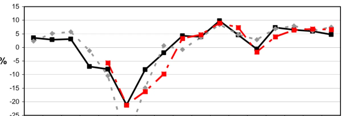
The development in Estonia is quite similar to the other two Baltic States, Latvia and Lithuania, as can be seen in Figure 2-1. The recovery after the independency was relatively strong and reliable even though the inflation was somewhat high. The privatisation, which started in 1992, was almost completed in 1999. Nonetheless, a problem arose in 1998 when the Russian economy collapsed. This forced the economy to change its trading partners which, to a large extent, had been Russia prior the economic collapse, but from now on became more EU-oriented. The Baltic people are known for having low wages which has and still gives incentives to a lot of multinational companies to start subcontractor factories there. This has been of great importance since the domestic market is weak. The education level, however, is a problem which slackens the speed of growth (Käbin, 1998). The prob-lem of urban growth and rural stagnation has been evident in the Baltic States as well as in the Central Eastern European countries.

4 _{If no other references are given, The Swedish Institute of International Affairs (2004) is used.}

Background

GDP Growth - Baltic States

-25 -20 -15 -10 -5 0 5 10 15 1987 1988 1989 1990 1991 1992 1993 1994 1995 1996 1997 1998 1999 2000 2001 2002 2003 Year %

Estonia Latvia Lithuania

Figure 2-1 GDP Growth in % - Baltic States.

Source: Data from World Development Indicators 2004, Calculations & graphics own production. Slovenia, Slovakia and Croatia had a harder starting position than for instance the Czech Republic and Poland. All three of them had different factors that had to be solved to reach a positive GDP growth. Slovenia was the richest of the republic states in Yugoslavia. The war did not affect them directly but a difficult problem arose after some years in the transi-tion process. The majority of the export had been to the former Yugoslavian states, but the Balkan war kept back almost all demand. Slovenia managed to find other trading partners, especially companies based in Germany. Slovakia was the poor part of Czechoslovakia and had problems getting the GDP growth positive until 1994. The GDP growth has been positive since then but unemployment, budget deficit and negative trade balance are prob-lems that were harder to solve. Croatia seems to have had the hardest time since the fall of the communists. It hade to take care of a disproportional large share of the debt from for-mer Yugoslavia, in addition the war affected Croatia in a direct way. The government had large problems to solve almost all important economic shortcomings that Croatia suffered from.

Theoretical Framework

3 Theoretical

Framework

3.1

The Solow Model

The neoclassical growth theory which is the basis of this thesis was first discussed in 1956 by Robert M. Solow in his article “A Contribution to the Theory of Economic Growth”. The following chapter is based on, Romer (2001), Dornbusch, Startz & Fischer (2004), Jones (2002), Barro and Sala-i-Martin (1999).

3.1.1 The Production Function

The exogenous growth theory is based on the assumption that technology is explained exogenously. In this model it assumed that there are two factors of production, capital (K) and labour (L). These two factors are used to produce output (Y), which gives that Y is de-pendent on K and L. The production function is written as follows:

)] ( ), ( [ ) (t =F K t L t Υ Equation 3-1

The output does not change over time (t) by itself. Variations in output must be due to changes, over time, in capital or labour. Another assumption that is crucial for the model is that the factors of production have positive but decreasing individually marginal productiv-ity. Nevertheless it is equally important that the production function experience constant returns to scale when employing both factors of production.

0 > ∂ ∂ K Y 0 2 2 < ∂ ∂ K Y 0 > ∂ ∂ L Y 0 2 2 < ∂ ∂ L Y ) , ( ) , ( K L F K L F λ λ =λ for all λ>0

If the production function is put in to a Cobb-Douglas form it looks as follows:

β α_L

K =

Υ Equation 3-2

where α + β = 1, which implies that the production has constant returns to scale. α is capi-tal’s share of total income and β is labour’s share.

The theory of the two factors of production also contains a quite a few assumptions. The characteristic of capital is dependent on the theory of saving and depreciation. The share of income that is not consumed is saved and written as “s”. The rate at which the capital de-preciates is symbolised with δ . Both s and δ are assumed to be constant and zero or posi-tive. Another assumption is that the economy is closed, hence, all capital saved is used for investment (sY = I). This implies that the change in the capital stock ( K& ) looks as follows:

K sY

K& = −δ Equation 3-3

The other input factor, labour, changes over time. Its growth rate is dependent on an ex-ogenous given constant; n, which is dependent on population, participation rates and inten-sity of work. The assumptions are that both participation rate and inteninten-sity of work are

Theoretical Framework

constant and equal to unity, hence if follows that the growth in labour only is dependent the population growth.

nt Le t

L( )= Equation 3-4

As can be seen from Equation 3-4 L(t) is assumed to exogenously grow exponentially.

3.1.2 Technology

The growth in capital and labour gives rise to growth in output according to Equation 3-1. However, in 1957 Solow published “Technical Change and the Aggregate Production Function” where he showed that technology had an impact on long run growth perform-ance. The technology level (A) is an exogenous variable which grow at rate g. How the technology enters the production function can be viewed in different ways. Either it is la-bour augmenting (also called Harrod-neutral) , capital augmenting (also called Solow-neutral β α_{( )} ) (t K AL Y =

5_{) , or Hicks-neutral . The difference}

is, as can be seen from the mathematical expressions, which factor of production the tech-nology improves. According to Barro and Sala-i-Martin it is only possible to work with a steady state model if the model is labour augmenting while Jones states that it is of less im-portance which expression you use if you are using a Cobb-Douglas function

β α_L AK t Y( )=( ) Y(t)= AKαLβ 6_{. In this} the-sis the productivity variable is assumed to be Hicks-neutral due the fact that new technol-ogy affects both the productivity of capital and labour.

3.2 Growth

Accounting

The crucial question is: can this theory analyse real world scenarios? Solow (1957) used a model which is based on the model he had written about a year earlier. What Solow inves-tigates in this paper are the factors behind the U.S.’s economic growth between 1909 and 1949. By using Equation 3-5; L L K K A A Y

Y& ₌ & _+α & _+β &

Equation 3-5

where α and β are the share of capital and labour in the production function respectively, he was able to estimate the technological growth (Romer, 1957). Since this figure is calcu-lated by estimating the error-term, it is sometimes called the “residual” or a “measure of our ignorance”. This formula has its origin in the production function written in Cobb-Douglas form. By writing the change in Y (Y& ):

) ( ) ( ) ( ) ( ) ( ) ( ) ( ) ( ) ( ) ( At t A t Y t L t L t Y t K t K t Y t

Y& & & &

∂ ∂ + ∂ ∂ + ∂ ∂ =

5 _{Not to be mixed-up with the model used in Solow’s “Technical Change and the Aggregate Production}

Function”.

6 _{For further reading in favour for Barro’s and Sala-i-Martin’s statement, see Barro & Sala-i-Martin, Chapter 1}

Theoretical Framework

This form shows that Y& is dependent on the change in each factor which is in their turn dependent on time. By dividing the equation with Y(t) and multiplying each part with

) ( ) ( t X t X

, (X is replaced with the specific factor) it is possible to estimate the input elasticises:

) ( ) ( ) ( ) ( ) ( ) ( ) ( ) ( ) ( ) ( ) ( ) ( ) ( ) ( ) ( ) ( ) ( ) ( ) ( ) ( t A t A t A t Y t Y t A t L t L t L t Y t Y t L t K t K t K t Y t Y t K t Y t

Y& & & &

∂ ∂ + ∂ ∂ + ∂ ∂ =

which can be written in a shorter form and is the same as Equation 3-5:

L L K K A A Y

Y& ₌ & _+α & _+β &

The assumption of constant returns to scale, results in α +β =1⇒β =1−α.

By using Equation 3-5 it is possible to estimate the contribution, of the included factors, to the growth in GDP.

3.2.1 Total Factor Productivity (TFP)

The technology factor (A) can also be called total factor productivity if A is seen as Hicks-neutral. This variable measure how effective the two input variables labour and capital are used in the production. Another way to express this variable is; how much Y per unit of K and L, see Equation 3-6. One explanation for the need to measure the TFP is when the quality or efficiency is increasing in either capital or labour or both (Metcalfe, 1997). This will not be seen in the figures of capital and labour input, but the output will increase. Thus, if the amount of labour and capital is constant and the GDP changes the explanatory factor for the change is TFP change.

A L K Y ₌ β α Equation 3-6

Nevertheless there are criticism against TFP and how to measure the variable. A famous example in this context is the expression that TFP is “a measure of our ignorance” (Abramovitz, 1956), which drastically shows one of the drawbacks of this model. The vari-able is not measurvari-able and thus the credibility is not as high as other measurvari-able varivari-ables. The calculated figure will include the actual TFP but also all ignored or missed variables not taken into account in the model as well as the measurement errors (Wang and Yao, 2001). However, deeper studies show that the importance of technology does not disap-pear when analysing input versus output further (Metcalfe, 1997).

Data

4 Data

The data in this thesis is brought from The World Bank’s The World Development Indicators 2004. The variables used are GDP, investments and labour. GDP is a variable that is widely used and is a comfortable way to measure how much that is produced in an economy. Nevertheless, there are important problems with this sort of measurement, especially in the countries examined in the thesis. First, the production in households is not measured and may vary between countries and time periods. The amount of households’ production is larger in developing countries than in industrialised (Parkin, Powell & Matthews, 2000). Since the post communist countries are somewhere in between developing and industrial-ised it is difficult to estimate the size of the households’ production. Second, the illegal market does not show up in the figures. This may cause a larger problem than the former since the black market and corruption is a problem in this region.

Employment data is hard to find expressed in the same unit as capital and GDP. Thus, the variable “wages and salaries” is used. A difficulty with using this variable is that the variable can change if the government changes the minimum wage. In addition the wage can in-clude the assumption that wages are equal to the marginal productivity of labour. Thus, if the labour becomes more productive wages will raise. The consequence is an increase in input which should instead have been a productivity growth. If labour measured in either man hours or in individuals the last assumption would be foregone. However, for simplic-ity all variables are measured in the unit standard. The change in wages and salaries should be proportional to the hour worked since the former is dependent on the later. In addition wages and salaries is the variable used when measuring GDP.

Finding reliable data on the capital stock is in general not an easy task, and has been par-ticular difficult for the region examined in this thesis. Other problems than just finding the data is the reliability (Jeurling, 1998). The difference to measure the capital stock in the post communist countries compared to measure in the western economies are that the already existing capital is very old in the former. The outcome is that the depreciation may be well over what is seen to be normal in western economies. The machinery may be totally useless since the communist regime used a different type of production strategy. In addition, the banking sector has been unstable, which may have resulted in reduced capital accessibility. Capital expenditure is used to measure the capital stock in the economies. It is assumed that capital expenditure in a country is proportional to the capital stock since it is close to impossible to measure the capital stock.

Estimations and Analysis

5

Estimations and Analysis

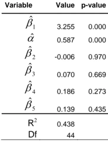
The data is a panel data set and the factor shares have been estimated by using Ordinary least-squares dummy variable regression model (LSDV), with GDP per capita as the de-pendent variable and capital per capita as the indede-pendent variable (Gujarati, 2003). The LSDV-model assumes an equal intercept for all years while the slope is individual. There are year specific dummies. Capital expenditure is assumed to be proportional the capital stock and the variable wages and salaries are assumed to be proportional to the labour stock. The data is from the nine countries examined between 1997 and 2001.

⎟ ⎠ ⎞ ⎜ ⎝ ⎛ + = ⎟ ⎠ ⎞ ⎜ ⎝ ⎛ ⎟ ⎠ ⎞ ⎜ ⎝ ⎛ = = Υ L K A L Y L K A L Y L AK ln ln ln α α β α given β = 1 - α

which according to above explained model gives:

it it it D D D D L K L Y _{β α +β +β +β +β +ε} ⎟ ⎠ ⎞ ⎜ ⎝ ⎛ + = ⎟ ⎠ ⎞ ⎜ ⎝ ⎛ 01 5 00 4 99 3 98 2 1 ln ln

Where β1 is the constant, D98, D99, D00 and D01 are year dummies and εit is the time and year specific error term. The capital’s share of the income (α) was estimated, and by assum-ing constant returns to scale (1 - α) also the labour share of income.

Table 5-1 Estimated values

Variable Value p-value

1 ˆ β _{3.255 0.000} αˆ 0.587 0.000 2 ˆ β _{-0.006 0.970} 3 ˆ β _{0.070 0.669} 4 ˆ β _{0.186 0.273} 5 ˆ β _{0.139 0.435} R2 0.438 Df 44 . 413 . 0 ˆ 587 . 0 ˆ = ⇒β = α

Capital’s share of income (αˆ ) is somewhat high compared with generally accepted values. The main factor is the problem in measuring capital. Other factors that may be important are the low wages and the high degree of FDI in these countries.

The shares are put into the formula below to find out the percentage change in technologi-cal growth.

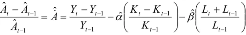
Estimations and Analysis ⎟⎟ ⎠ ⎞ ⎜⎜ ⎝ ⎛ + − ⎟⎟ ⎠ ⎞ ⎜⎜ ⎝ ⎛ − − − = = − − − − − − − − − 1 1 1 1 1 1 1 1 ˆ _ˆ ˆ ˆ ˆ ˆ t t t t t t t t t t t t L L L K K K Y Y Y A A A A _{& α β}

The values in Table 5-2 are based on t and t-1 being 2001 and 1996 respectively. The change in capital and wages include factors shares, estimated above.

Table 5-2 Factor growth 1996 – 2001

Country Hungary Poland Estonia Latvia Lithuania Czech

Republic Slovak Republic Slovenia Croatia GDP 24.7% 22.4% 30.4% 34.6% 24.9% 5.0% 17.5% 22.7% 15.9% Capital 25.2% 12.8% -17.0% 44.7% 29.8% -7.2% 4.7% 9.4% -24.3% Wages 15.4% -13.2% -6.9% -4.0% 10.4% 0.2% 0.9% 13.0% 8.0% TFP* -15.9% 22.8% 54.3% -6.0% -15.4% 12.0% 11.9% 0.3% 32.1% TFP (% of GDP)* -64.2% 101.9% 178.8% -17.3% -61.8% 239.7% 68.0% 1.3% 202.6%

Source: Data from World Development Indicators 2004. *Calculations based on estimations made in this thesis.

As can be seen in Table 5-2, the GDP has been positive in all investigated countries during the period. At the same time the factor accumulation differs to a large extent. Poland, Es-tonia and the Czech and Slovak Republics as well as Croatia have had negative growth in either capital, labour or both factors. Despite this, their GDP growth has been positive which implies a more effective usage of the factors remaining. Thus, the TFP growth is positive. Hungary, Latvia and Lithuania have all hade negative TFP growth. Their factor accumulation has been larger than they have had technology for. They have succeeded in collecting the capital and labour, but they had problems using this extra input in an effi-cient way. This is a pattern similar to the growth for the Asian Tigers. Hence, the impor-tance of looking beyond the numbers of GDP growth is essential. Even though the output has developed in the same direction and also in the same magnitude; the underlying factors differ.

Critics may argue that the productivity growth has not shown any similarities in three of the more or less arbitrary sorted groups. The results vary in a large scale and the TFP growth seems to be more dependent on variations in the input variables. One example is Poland in 1998, where wages decreased by 39 per cent, in addition the capital expenditure fell by 29 per cent (The World Bank Group, 2004). At the same time the GDP rose by 4 per cent. The following years, wages and capital expenditures slowly climbed up again but never reached the high levels in 1998, while GDP kept on growing with approximately 4 per cent annually. The outcome is an increase in TFP. Table 5-3 gives an annual figure of the TFP-growth between 1994 and 2001.

Estimations and Analysis

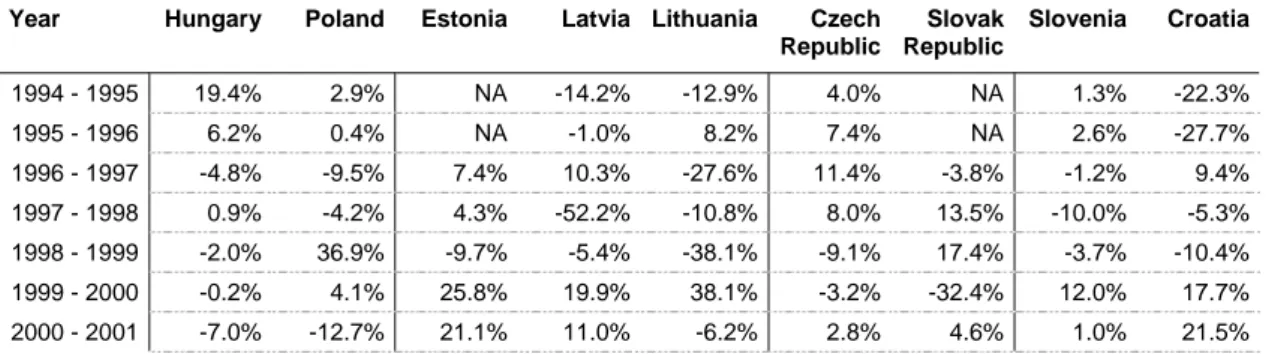
Table 5-3 TFP between 1994 and 2001

Year Hungary Poland Estonia Latvia Lithuania Czech

Republic Slovak Republic Slovenia Croatia 1994 - 1995 19.4% 2.9% NA -14.2% -12.9% 4.0% NA 1.3% -22.3% 1995 - 1996 6.2% 0.4% NA -1.0% 8.2% 7.4% NA 2.6% -27.7% 1996 - 1997 -4.8% -9.5% 7.4% 10.3% -27.6% 11.4% -3.8% -1.2% 9.4% 1997 - 1998 0.9% -4.2% 4.3% -52.2% -10.8% 8.0% 13.5% -10.0% -5.3% 1998 - 1999 -2.0% 36.9% -9.7% -5.4% -38.1% -9.1% 17.4% -3.7% -10.4% 1999 - 2000 -0.2% 4.1% 25.8% 19.9% 38.1% -3.2% -32.4% 12.0% 17.7% 2000 - 2001 -7.0% -12.7% 21.1% 11.0% -6.2% 2.8% 4.6% 1.0% 21.5%

Source: Data from World Development Indicators 2004.

When the communist regime fell, a large share of government supported industries had to close due to their inefficiency (The Swedish Institute of International Affairs, 2004). The result was a loss of knowledge and technology. This can be one of the explanations why the TFP-growth is negative in the beginning of the transition for a number of the coun-tries. The industry had to find new markets and other production methods, hence before the new industries where working as they where meant to be the productivity where lower than before the transition. A similar pattern for all countries studied is a second slump in the TFP-growth. The first drop occurred directly after the political change while the second downturn is most likely explained by regional factors. One factor explaining the drop in the Baltic States is the crisis in Russia in 1998. Before 1998 they were all strongly dependent on the Russian economy, but after the economic crisis in Russia they were forced to turn to other markets, where there was a demand for other products. Thus, capital and knowledge had to be thrown away and new production systems had do be build. The drop in TFP is il-lustrated in Figure 5-1.

TFP-growth in the Baltic States between 1995 - 2001

-5.0% -4.0% -3.0% -2.0% -1.0% 0.0% 1.0% 2.0% 3.0% 4.0% 5.0% 1994-1995 1995-1996 1996-1997 1997-1998 1998-1999 1999-2000 2000-2001 Year % c h a nge in TFP

Estonia Latvia Lithuania

Figure 5-1 TFP-growth in the Baltic States, between 1995 and 2001.

Source: Data from World Development Indicators 2004, calculations & graphics own production.

Conclusion and Further Research

6

Conclusion and Further Research

What is found in this thesis is that the GDP is only one of many important factors to ana-lyse when scrutinizing the economic development in Central Eastern Europe and the Baltic States. The growth has in some countries been dependent on factor accumulation while other countries have had a TFP growth. Furthermore, the productivity growth has been varying over time which can be explained by the dependence on infrastructure investments. These investments were to a large extent financed from abroad and varied from year to year. The countries with a GDP growth driven by factor accumulation should not be sur-prised if the growth suddenly cease. These countries have to turn their growth into TFP dependent.

During the work with this thesis the importance of time span in a study like this, has been brought up to surface. The problem that arises is that there is hard to see any trends, and if some trends may be observed they may just be deviations from a larger trend. External shocks may influence the results in a study when the time span is shorter compared to a study with a longer time periods. This fact gives future students an opportunity to examine whether there are any similarities between the growth in East Asia and the post communist countries when looking in a longer time perspective. Other factors affect, according to the-ory and empiric studies, the GDP growth. To examine for example whether corruption, educational level, intersectoral reallocations and labour are included in the residual, would be an interesting continuation of this thesis.

Reference List

Reference List

Abramovitz, M. (1956). Resource and Output Trends in the United States since 1870. American Economic Review, Papers and Proceedings. 46, 5-23.

Barro, R. J., & Sala-i-Martin, X. (1999). Economic Growth (2nd _{ed.). Cambridge MA.: MIT} Press.

Borg, M. (1998). Bidrag till utvecklingen av Östersjöregionen. In L. Borg (Ed.), De Baltiska Tigrarna (p. 31-36). Laholm: Svenska Arbetsgivareföreningen.

Dornbusch, R., Startz, R., & Fischer, S. (2004). Macroeconomics (9th _{ed.). Boston MA:} McGraw-Hill/Irwin, cop..

Edwards, S. (1997). Openness, Productivity and Growth: What do we really know?. NBER Working Paper Series. 5978.

European Bank for Reconstruction and Development, (2003). Transition report 2003, Integra-tion and regional cooperaIntegra-tion. London: EBRD PublicaIntegra-tion Desk.

Gujarati, D. N. (2003). Basic Econometrics (4th _{ed.). New York NY: McGraw –Hill/Irwin.} Jeurling, L. (1998). Läget i Baltikum: Ekonomi och politik. In L. Borg (Ed.), De Baltiska

Tig-rarna (p. 31-36). Laholm: Svenska Arbetsgivareföreningen.

Jones, C. I. (2002). Introduction to Economic Growth (2nd _{ed.). New York NY: W.W Norton.} Kozminski, A. (2002). Economies of central and eastern Europe, transition of. In Warner,

M. (ed.), International Encyclopaedia of Business and Management (p. 1598 – 1576). London: Thomson Learning.

Krugman, P. (1994). The Myth of Asia’s Miracle. Foreign Affairs. 73(6), 62-78.

Käbin, T. (1998). Det baltiska näringslivet: Svenska handels- och etableringsmöjligheter. In L. Borg (Ed.), De Baltiska Tigrarna (p. 37-42). Laholm: Svenska Arbetsgivarefö-reningen.

Metcalfe, J. S. (1997). The evolutionary explanation of total factor productivity growth: macro measurement and micro process. CRIC Discussion Paper. 1.

Noorikôiv, R., Orazem, P. F., Puur, A., & Vodopivec, M. (1998). Employment and Wage Dynamics in the Estonia Transition, 1989 – 1995. Economics of Transition. 6(2), 481-503.

Parkin, M., Powell, M., & Matthews, K. (2000). Economics (4th _{ed.). Barcelona:} Addison-Wesley.

Romer, D. (2001). Advanced Macroeconomics (2nd _{ed.). Boston MA: McGraw-Hill.}

Solow, R. M. (1956). A Contribution to the Theory of Economic Growth. The Quarterly Journal of Economics. 70(1), 65-94.

Reference List

Solow, R. M. (1957). Technical Change and the Aggregate Production Function. The Review of Economics and Statistics. 39, 312-320.

Swedish Institute of International Affairs, The. (2004, December 4). Landguiden. Retrieved December 3, 2004, from http://www.landguiden.se/

Wang, Y., & Yao, Y. (1999). Source of China’s Economic Growth, 1952-99; Incorporating Human Capital Accumulation. The World Bank, Policy Research Working Paper Se-ries: 2650.

World Bank Group, The. (2004). World Development Indicators 2004 [Computer Soft-ware] Washington, DC: The World Bank Group.

Young, A. (1994). The Tyranny of Numbers: Confronting the Statistical Realities of the East Asian Growth Experience. NBER Working Paper No. 4680.