Implementing a New Register Allocator for the Server Compiler in the Java HotSpot Virtual Machine

(1)

UPTEC IT 15011

Examensarbete 30 hp

Juni 2015

Implementing a New Register

Allocator for the Server Compiler

in the Java HotSpot Virtual Machine

Niclas Adlertz

(2)

(3)

Teknisk- naturvetenskaplig fakultet UTH-enheten Besöksadress: Ångströmlaboratoriet Lägerhyddsvägen 1 Hus 4, Plan 0 Postadress: Box 536 751 21 Uppsala Telefon: 018 – 471 30 03 Telefax: 018 – 471 30 00 Hemsida: http://www.teknat.uu.se/student

Abstract

Implementing a New Register Allocator for the Server

Compiler in the Java HotSpot Virtual Machine

Niclas Adlertz

The Java HotSpot Virtual Machine currently uses two Just In Time compilers to increase the performance of Java code in execution. The client and server compilers, as they are named, serve slightly different purposes. The client compiler produces code fast, while the server compiler produces code of greater quality. Both are important, because in a runtime environment there is a tradeoff between compiling and executing code. However, maintaining two separate compilers leads to increased maintenance and code duplication.

An important part of the compiler is the register allocator which has high impact on the quality of the produced code. The register allocator decides which local variables and temporary values that should reside in physical registers during execution. This thesis presents the implementation of a second register allocator in the server compiler. The purpose is to make the server compiler more flexible, allowing it to produce code fast or produce code of greater quality. This would be a major step towards making the client compiler redundant.

The new register allocator is based on an algorithm called the linear scan algorithm, which is also used in the client compiler.

The implementation shows that the time spent on register allocation in the server compiler can be greatly reduced with an average reduction of 60 to 70% when running the SPECjvm2008 benchmarks. However, while the new implementation, in most benchmarks, is slower than the register allocator in the client compiler, concrete suggestions on how to improve the speed of the new register allocator are presented.

Looking at performance, the implementation is not yet in line the with the client compiler, which in most benchmarks produces code that performs 10 to 25% better. The implementation does, however, have good potential in reaching that performance by implementing additional performance improvements described in this thesis. The benchmark data shows that, while the new implementation looks promising, additional work is needed to reach the same compilation speed and performance as the register allocator in the client compiler. Also, other phases in the server compiler, such as certain optimization phases, also need to be optional and adjustable to further reduce the compilation time.

Ämnesgranskare: Tobias Wrigstad Handledare: Nils Eliasson

(4)

(5)

Introduction

1.1 The Java Execution and Runtime

Java code is executed using a program called a Java Virtual Machine (JVM). When compiling Java code, one or more class files are created. Class files contain what is called Java bytecode, which is a compact platform independent repre-sentation of the Java code. Platform independency is one of the main features of Java.

The JVM runs the Java program by interpreting the Java bytecode. Interpre-tation of Java bytecode is a straightforward approach, but it is slow. In order to increase the performance of a Java program, the JVM can compile the Java bytecode to native platform dependent machine code at runtime. This is called Just In Time (JIT) compilation. By compiling Java bytecode to machine code, it can execute directly on the platform without having to be interpreted by the JVM.

JIT compilation however is time consuming, and there is a tradeoﬀ between compiling and interpreting Java bytecode. If some part of the Java bytecode is not executed frequently enough is not worth JIT compiling. The most common JVM today is developed by Oracle and is named the Java HotSpot Virtual Machine. It keeps track of the invocation count of all methods in the Java program that is being executed. Once a method of the Java program has been invoked enough times, is considered to benefit from JIT compilation. In the Java HotSpot VM that invocation threshold is currently 200.

The Java HotSpot VM currently has two JIT compilers; the Java HotSpot client compiler and the Java HotSpot server compiler. The client compiler does not apply as many optimizations as the server compiler to the code that is being compiled and because of this the client compiler spends less time during compilation. The client compiler produces less eﬃcient code compared to the server compiler in general. There are plenty of times when the produced code of the client compiler is eﬃcient enough for a particular method or application. However, if an application is designed to run for a long time and handle many

(8)

computations, such as many server applications, it is more important to have high quality code, and for this the server compiler is a better alternative.

1.2 Two JIT Compilers in the HotSpot VM

One big issue with having two JIT compilers are the separate code bases. The JIT compilers have been written separately and share a minimal amount of code, if any. This has historical reasons as the two compilers were initially developed by diﬀerent companies. Having two JIT compilers means increased maintenance and a lot of code duplication. One solution to this problem is to use a single JIT compiler with the ability to choose the level of optimization to apply to the Java bytecode that is being compiled.

One of the most important steps in the compilation process is register allocation. It will be explained in more detail later on, but in short it is the step that assigns local variables and temporary values to physical registers in the computer. This step can be time consuming but also has a high impact on the quality of the produced code, as accessing data in registers is faster than accessing data in memory. The client compiler uses a faster register allocator algorithm than the server compiler, but in general it produces less eﬃcient code.

1.3 The Goal of This Thesis

The goal of this work is to take a first step in exploring the possibility of re-moving the client compiler by allowing the server compiler to perform faster compilations. Concretely, this work consists of designing and implementing a new register allocator for the server compiler that is able to produce code with a quality on par with, and in the same time-frame as, the client compiler’s register allocator.

1.4 Outline

This thesis starts by first covering necessary JVM and compiler related topics in Chapter 2. Register allocation in general is described in Chapter 3 and the current register allocation algorithms used in the client and server compilers are then described in Chapter 4 and Chapter 5. This is followed by Chapter 6 which covers the implementation of the register allocation algorithm used for this thesis. In Chapter 7 tests and results are shown and evaluated. Future work is covered in Chapter 8 and Chapter 9 concludes.

(9)

Chapter 2

Background

This section explains Java bytecode and JIT compilation as well as compiler related keywords that the reader needs to be familiar with in order to understand later parts of this report.

2.1 Java Bytecode

One of the major design goals of Java is that programs written in Java should be cross-platform. This means that one should be able to write a Java pro-gram on one platform and execute the propro-gram on another platform, without any modifications to the code and without having to recompile the program. In practice this means that when a Java program is compiled into class files, the class files will contain a platform-independent instruction set called Java bytecode. In order to run a Java program on a specific platform, a compliant JVM must be developed for that platform. A JVM is a program that is able to execute programs that are compiled to the Java bytecode instruction set by translating the Java bytecode into native machine instructions of the platform at hand.

The Java bytecode is a more compact representation of Java code in the form of instructions that the JVM executes. An instruction can be as short as one byte, although many Java bytecode instructions have additional arguments, adding a few bytes to the instructions. The Java bytecode instruction set is stack-oriented, which means that it does not use any registers. Instead everything must be pushed to a stack before it can be used in a calculation. In order to demonstrate how bytecode is structured, consider a regular Java method shown in Figure 2.1.

(10)

static int add(int a, int b) { return a + b;

}

Figure 2.1: A simple add method in Java.

Figure 2.2 shows the same method compiled into Java bytecode. The method consists of four Java bytecode instructions, each instruction is one byte in size. Two values are pushed onto the stack, load_0 and iload_1. The add instruction pops the two operands and pushes the result from the addition onto the stack which is then popped by the return instruction.

0: iload_1 1: iload_2 2: iadd 3: ireturn

Figure 2.2: The compilation of the method in Figure 2.1.

In the Java HotSpot VM the Java bytecode instructions are processed one by one, by implementing a stack based machine. Each time a method is invoked, the Java bytecode instructions for the method are interpreted and the stack machine is used to store results and variables for future use. If the same method is called again, it has to be interpreted once again. The interpretation acts as an layer on top of the architecture. It does not have to know anything about the hardware it is running on. And even though this is a key component of Java’s platform independence, interpretation makes execution slow.

2.2 JIT Compilation

In order to improve the execution time the Java bytecode is compiled to native machine code to avoid the performance overhead of the interpretation. Instead of interpreting the Java bytecode, it is compiled into instructions that the hard-ware is familiar with. In order to preserve the cross-platform requirement, this is not done prior to execution, since that would make the code platform-dependent. Instead JIT compilation is used, meaning that the Java bytecode is compiled to native code at runtime, while the Java HotSpot VM is running. The downside to dynamic compilation is that the time it takes to compile a method could be

(11)

spent on interpreting code instead. JIT compilation is a time consuming task, so in order for JIT compilation to be benefitial, the code that is compiled has to be executed frequently.

In other words, the cost C of compiling a method M to machine code can be amortized over all invocations N of the method, and if the time it takes to interpret M is IM and the time it takes to execute the compiled version of M is CM, then the goal is to satisfy C + N * CM <= N * IM. Otherwise, the system has been made slower due to the JIT compilation.

As mentioned earlier there are two JIT compilers for the Java HotSpot VM, the Java HotSpot VM client compiler and the Java HotSpot server compiler. While the client compiler is faster than the server compiler, the client compiler does not produce code of the same quality as the server compiler. The client com-piler is suitable when low startup times and responsiveness are important. The server compiler on the other hand is suitable for long-running high performance applications, such as typical server applications.

2.3 Intermediate Representations

When a compiler translates source code written in one computer language into another one, in this case from Java bytecode to machine code, the compiler uses one or more intermediate representations of the source code during the compilation process.

There are several reasons why to use intermediate representations. One is that a compiler can compile programs written in diﬀerent languages, as long as the pro-grams have been converted to an intermediate representation supported by the compiler. An example of this is the LLVM infrastructure with its intermediate representation named LLVM IR [1].

The intermediate representations can be divided into diﬀerent levels of abstrac-tion. Low-level intermediate representations are closer to machine code. This facilitates platform-specific optimizations. High-level intermediate representa-tions are usually platform independent and give a better view of the control flow of methods since the platform dependent details are omitted. High-level intermediate representations also enable more general optimizations such as Constant folding, Common subexpression elimination and loop optimizations [2].

2.4 Control Flow Graph

A control flow states the order in which statements and instructions are executed or evaluated.

A very common intermediate representation is a Control Flow Graph (CFG). A CFG consists of basic blocks. A basic block is a continuous sequence of instructions without jumps or jump-targets in the between. This means that

(12)

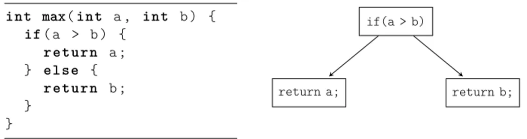
only the last instruction in a block can be a jump to one or more basic blocks. In Figure 2.3 a Java method is shown and illustrated using a CFG.

int max(int a, int b) { if(a > b) { return a; } else { return b; } } if(a > b) return a; return b;

Figure 2.3: A simple Java method and its corresponding CFG.

The CFG is an important representation that is used throughout the compilation process, in particular in the liveness analysis (which will be explained later in this chapter) used for register allocation.

2.5 Static Single Assignment Form

A property used often in intermediate representations is the Static Single As-signment (SSA) form. This means that each variable is only defined once and it simplifies a lot of optimizations that the compiler is doing, including liveness analysis. Figure 2.4 illustrates how a simple Java code snippet is converted into SSA form. When a variable is assigned more than once, a new variable is created replacing all later uses of the original variable.

(13)

y = a + x; ... y = c; ... a = y; Non-SSA form. y1 = a + x; ... y2 = c; ... a = y2; SSA form. Figure 2.4: Code represented in SSA form.

However, there are situations where this notation is not suﬃcient. Consider another example in Figure 2.5. Both assignments of y have already been replaced with unique variables y1 and y2. But which y will be used in the assignment of g in g = f + y?

y1 = a; y2 = b;

g = f + y?

Figure 2.5: Problem with SSA notation at a control flow merge.

The problem arises because of a merged control flow with assignments to the same variable in multiple branches. This is solved by adding a special statement, a φ(Phi)-function. The φ-function takes all the diﬀerent definitions of a variable as input (in this case y). As shown in Figure 2.6 the φ-function will be added in the beginning of the last block. It will generate a new variable y3, that represents either y1 or y2. This way, the intermediate representation is still on SSA form.

y1 = a; y2 = b;

y3 = φ(y1,y2) g = f + y3

(14)

2.6 Liveness Analysis and Live Ranges

Liveness analysis determines which variables are live at a certain program point in the CFG. If a variable V at a certain program point P is used later in the code, the variable V is live at P, otherwise the variable V is dead at P. For each variable, a live range is calculated. A live range represents at which program points in the code that a variable is live. In its simplest representation, a live range starts at a variables first definition and ends at its last use.

In order to do certain optimizations such as dead code elimination and more importantly, in the context of this thesis, to do register allocation, liveness analysis is needed. This will be obvious in later chapters.

Liveness can be calculated with diﬀerent quality. A less precise liveness is faster to compute, but may result in poorer quality of the produced code. This means that some variables that might not be live, are still displayed as being live, because the liveness analysis is less precise. The downside to this is that more variables maybe be considered live at the same time, which may as a consequence result in reduced code quality of the produced code.

(15)

Chapter 3

Register Allocation

A computer has a limited number of hardware registers, also called physical registers. They are the fastest accessible memory locations inside the computer. Most hardware instructions can only access operands that reside in physical registers. The register allocator determines which variables in the source code that should reside in physical registers at every specific program point.

If there are more variables and temporary values, also called virtual registers, live at a certain program point than there are physical registers, then some of the virtual registers need to be moved to a lower level in the memory hierarchy. This is called spilling. Spilling a variable to memory and restoring it to a physical register later on is associated with a cost. Therefore, the main task of the register allocator is to reduce the number of spills. Deciding whether or not a method with N virtual registers can be assigned to X number of physical registers, without performing any spilling, is NP-complete. This was proven by Chaitin when he showed that register allocation is equivalent to a NP-complete problem called graph coloring [5]. Since the problem is NP-complete, the register allocator computes an eﬀective approximate solution to the problem.

There are several approaches to the register allocation problem. Since a JIT compiler is compiling code at runtime, the demands on the JIT compiler are diﬀerent than for a static compiler (i.e. a compiler compiles the entire program into native code before executing it). The JIT compiler has to be fast, since time is crucial when compiling at runtime. The extra overhead to produce higher-quality machine code might not speed up the overall execution of the program. Instead, a trade-oﬀ between code quality and compilation time must be made. Besides choosing a proper algorithm for register allocation, it can also be applied locally or globally.

3.1 Local Register Allocation

Local register allocation looks at part of the code, usually a block in a CFG or the innermost loops in a method. It assigns registers to the variables within that block or loop and then spills everything that resides in registers to memory

(16)

in between blocks. In order to do local register allocation, liveness analysis has to be done for each block. Local register allocation algorithms are very fast, but since the register allocation is only done per block or to a region of blocks, spilling has to occur in between those regions. Location register allocation could be suitable when compiling methods in multiple tiers. When a method is first compiled, the register allocation could be done locally to reduce the compilation time. At a later stage in execution, if the method is still frequently used, it could be recompiled, this time using global register allocation.

3.2 Global Register Allocation

Global register allocation spans over many blocks at a time, usually on a com-plete method (or even several methods that might have been inlined). This approach generates less spilling, but is also more time consuming than doing local register allocation. A liveness analysis stage is needed, which gathers in-formation about where all the virtual registers in a method are live, i.e. where they need to reside in a physical register or in memory. Also, some machine instructions require specific physical registers, so liveness information about the physical registers may also have to be acquired.

Both the client compiler and the server compiler use global register allocation algorithms. The server compiler treats the register allocation problem as a graph coloring [5] problem. The client compiler uses another approach, called second chance binpacking [3] which originates from the linear scan algorithm [4]. All of these approaches will be covered later on.

(17)

Chapter 4

Register Allocation using

Graph Coloring

The current register allocation algorithm in the Java HotSpot VM server com-piler is based on work first presented by G.J. Chaitin [5]. It uses a graph that consists of nodes connected by edges. A finite number of colors are also intro-duced. Each node in the graph is assigned a color, but nodes that are adjacent,

i.e. connected with an edge, can not be assigned the same color. If all nodes

can be assigned colors, without two connected nodes having the same color, the graph is said to be colorable. This technique is called graph coloring.

When graph coloring is used for register allocation, each node in the graph cor-responds to live range of a virtual register in the method that is being compiled. As explained in Chapter 2, a live range represents at which program points in the method that a variable is live. The edges in the graph represent live ranges that are live at the same time, and the colors represents the number of physical registers available. If two virtual registers are live at the same time, they cannot get assigned the same physical register.

The nodes and edges are represented using an interference graph, as shown in Figure 4.1. Each node corresponds to a live range, which in turn corresponds to a virtual register. The edges between the nodes show which live ranges that are live at the same time.

(18)

1 2

3 4

Figure 4.1: An interference graph consisting of four nodes and four edges.

Figure 4.1 shows that nodes 1, 2 and 3 cannot be assigned the same color. Also nodes 3 and 4 cannot be assigned the same color. However, node 4 can be assigned the same color as nodes 1 and 2 since node 4 is not directly connected to either node 1 or 2.

4.1 Pruning the Interference Graph

In order to color the graph, i.e. assign physical registers to the live ranges, each node is pruned from the interference graph and pushed onto a stack. The stack represents in which order the nodes should be assigned a physical register. There are two rules that can be used when pruning nodes from the graph:

1. If the graph contains a node with less edges than the number of R registers, then it is colorable if and only if the graph without this node is R-colorable. The nodes that satisfy the first rule will not make an R-colorable graph un-colorable by being added. Therefore they are trivial and pruned first.

2. If there are any remaining nodes that do not satisfy the condition of the first rule at least one of them has to be pruned using a cost-function. The task of a cost-function is to select a node that will have the least impact on performance, since the node pruned by this rule is a potential spill node. The spilled node will reside in memory.

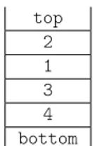
If all nodes are removed by using the first rule, the graph is guaranteed to be colorable. Looking at the interference graph in Figure 4.1 and having R = 2 number of physical registers, only node 4 would initially get selected by the first rule. The next node to be pruned would have to be chosen by using a cost-function.

If the cost-function would choose node 3, both the remaining nodes 1 and 2 could be removed by using the first rule. Figure 4.2 shows how that stack would look.

(19)

top 2 1 3 4 bottom

Figure 4.2: An example of a pruned interference graph.

4.2 Reconstructing the Interference Graph

Once all the nodes have been pruned from the interference graph, one node at a time is popped from the stack. Each popped node is inserted into the interference graph and its edges are added. The added node is also assigned a physical register that is not yet used by an adjacent node. If all nodes are assigned a physical register then no spilling is needed and the register allocation is complete. However, if no physical register is available when a node is inserted into the interference graph, the node is marked as a spill node. This means the node has to be spilled to memory.

When all nodes are re-inserted into the interference graph and one or more nodes are marked as spill nodes, additional spill code has to be inserted into the intermediate representation. The graph coloring algorithm is then repeated, because of the new the spilling code that has to be added also needs registers. This is repeated until no more spilling is required.

Even though there are ways of reducing the number of virtual registers, for example by using a technique called coalescing [5] (where live ranges that does not interfere are combined), the asymptotic time complexity of the algorithm always remains O(n2_{), where n is the number of virtual registers. Also, the}

(20)

Chapter 5

The Linear Scan Algorithm

The Java HotSpot client compiler uses an algorithm that is not based on graph coloring. Instead it is based on the linear scan algorithm [4]. It assigns physical registers to virtual registers in a single pass. This means it is much faster than the general graph coloring algorithm yet still produces relatively good code [4].

5.1 Block Order, Row Numbering and Intervals

The linear scan algorithm operates on a list of intervals. An interval is another name for a live range of a virtual register. In order to build all the intervals, the blocks in the CFG are ordered and added to a list where each instruction inside each block is assigned a global unique row number. Each virtual register V is assigned an interval starting at the first definition of V and ending at the last use of V. Figure 5.1 shows the definition of the virtual register x. x is defined at row number 11 and last used at row number 14. Assuming x is not re-defined anywhere else and not used after row number 14, the interval of x is defined as the range from 11 to 14.

10 ... 11 x = y + z; 12 a = x + 2; 13 b = z + 2; 14 c = x + 1; 15 d = a + c; 16 ...

(21)

The block order that the linear scan is operating on is important for improving the performance of the compiled code. A good block order may lead to shorter intervals, which leads to fewer variables being live at the same time. A good block order also orders blocks that are part of a loop to be adjacent in the linear block list, and blocks belonging to nested loops both to be adjacent and in between the outer loop blocks.

5.2 Assigning Physical Registers to Virtual

Reg-isters

Now that each virtual register has an interval, physical registers are assigned to all intervals. All intervals are put in a list named unhandled which is sorted on increasing start-point. When the unhandled list is empty, the algorithm has finished, and all the intervals (which corresponds to virtual registers) have either been assigned a physical register or a memory position.

There is also a second list, the active list, which contains live intervals that are already assigned a physical register. The active list is also sorted on increasing end-point in each iteration.

In each iteration, the algorithm first retrieves an interval from the unhandled list, this is the current interval. The current interval is then used to determine if any intervals in the active list are not live anymore, i.e. intervals whose end-points are before the current interval’s start-point. If there are any intervals in the active which are not live anymore, they are removed from the active list and their assigned physical registers are marked as available again.

If the number of active intervals are equal to the physical number of registers R that are available, the current interval or an interval from active list is assigned a spilled slot. There are many ways of choosing which interval to assign a spill slot. In this example, the interval with the last end position is spilled. If the chosen interval resides in the active list, it is removed and its previously assigned register is assigned to the current interval, the current interval is then added to the active list.

If the number of live intervals are less than the number of available physical register R, the current interval is assigned a free register and added to the active list.

(22)

function LinearScanRegisterAllocation() for Interval iv in unhandled

ExpireOldIntervals (iv)

if active . length == R

SpillAtInterval (iv)

else

iv. register = freeRegisters . first () active .add (iv)

active . sort ()

function ExpireOldIntervals( Interval iv) for Interval aiv in active

if aiv. endPoint >= iv. startPoint return

active . remove (aiv )

freeRegisters .add(aiv. register )

function SpillAtInterval( Interval iv)

Interval siv = active . last ()

if siv. endPoint > iv. endPoint

iv. register = siv . register

siv . register = newStackLocation () active . remove (siv )

active .add (iv) active . sort ()

else

iv. register = newStackLocation ()

Figure 5.2: The linear scan algorithm.

5.3 Resolve Stack Intervals

If one or more intervals are assigned memory positions, additional spill code is needed. Figure 5.3 gives an example of this. The value V of an interval that is residing in memory at position M1 is used in an addition. However, before V can be used it needs to be moved to a register. In this example it is moved to register R3. Before moving the value of M1 to R3, the current value in R3 must be saved to memory. The value of R3 is saved to memory position M2. Once the addition is complete, the old value of R3 is restored.

(23)

R1 = M1 + R2;

Memory + register addition.

M2 = R3 R3 = M1 R1 = R3 + R2 R3 = M2

Register + register addition. Figure 5.3: Stack interval resolving.

The need to operate directly on registers is partly true. On the x86 and x86-64 platform, there are several instructions that can operate directly on variables that reside in memory.

5.4 Lifetime Holes

The Java HotSpot VM client compiler extends the linear scan algorithm. The liveness analysis is more exact which means intervals now may contain lifetime holes. Lifetimes holes can occur if there are one or more blocks between blocks that the virtual register is live in. This can happen because the blocks are in a linear list.

When redefining a virtual register, the old value is dead between the last use of the old value and the redefinition. Figure 5.4 shows that variable x has two live ranges, one from row 11 to row 12 and one from 14 to 15. x is dead at row 13 because of the redefinition at row 14. Without support for lifetime holes, x would have only one live range starting at row 11 and ending at row 15.

10 ... 11 x = y + z; 12 a = x + 2; 13 b = z + 2; 14 x = y + 3; 15 d = x + c; 16 ...

Figure 5.4: The virtual register x with lifetime holes.

The benefit of lifetime holes is that a physical register being used by an interval is available for other intervals during its lifetime holes, which may reduce the

(24)

spilling. In order to know when an interval is dead due to a lifetime hole, an extra list has to be added to the algorithm, the inactive list, which keeps all the intervals that have been assigned a register but are inactive at the current interval.

5.5 Interval Splitting

Another added feature in the Java HotSpot VM client compiler is interval split-ting. This means that an interval may reside in a register at one point and in memory at another point. Interval splitting may reduce the spilling but it introduces non-linear parts in the algorithm.

(25)

Chapter 6

Implementing the Linear

Scan Algorithm in the

Server Compiler

6.1 The Intermediate Representation in the Server

Compiler

The server compiler uses a dependency graph [6] as an intermediate representa-tion, where each node in the dependency graph represents an instruction. Each node can produce a value based on an operation and its input. Values produced by nodes are used as input to other nodes. Figure 6.1 shows how two nodes representing an integer division and an integer addition have previously defined nodes as inputs. int 1 int 2 idiv 4 int 3 iadd 5

Figure 6.1: Nodes are instructions and edges are the relations between them.

A dependency graph diﬀers from a CFG in the way that it does not consist of blocks with sequential lists of instructions. Instead the instructions (called

(26)

nodes) are floating; meaning they do not belong to a block and do not have a fixed order. This makes optimizations involving code motion easier [6].

However, when entering the register allocation step in the server compiler, the intermediate representation is converted to a CFG. In order for the original register allocation algorithm in the server compiler to operate properly, the nodes need to be represented as a CFG. This is also the true for the linear scan algorithm.

The ordering of blocks is taken care of by the server compiler. When it creates the CFG, it orders the blocks in a list. The block list keeps blocks within a loop adjacent. It also keeps blocks of nested loops in between blocks of outer loops. The order of the block list is used as the block order when assigning row numbers to the nodes and building the intervals for the implementation of the linear scan algorithm in the server compiler.

6.2 Mapping Nodes to Machine Instructions

Before the dependency graph is converted to a CFG, the code has been heavily optimized and all nodes representing actual instructions have been converted into MachNodes. MachNodes map to machine instructions on the targeted plat-form. All MachNodes have a corresponding bitmap describing in which phys-ical registers the value of the MachNode can resign, this bitmap is called the outRegMask. Each node also has a specific bitmap of registers for each data input slot, called the inRegMask.

On the x86-64 platform there are 16 general purpose registers (GPR) 1_{. In}

addition to the 16 GPR registers there are also 16 floating point registers (XMM) namely XMM0 - XMM15. The XMM registers are used mainly for floating point computations.

6.2.1 Fixed Registers

On the x86-64 platform, some instructions operate only on certain, fixed, reg-isters. For example, when dividing two integers on the x86-64 platform, the numerator has to be in register RAX. Similarly, the value of an operation can also be bound to a fixed register. When dividing two integers, the produced value is always put in register RAX.

Figure 6.2 shows which registers that can be used to store a value for a node. The possible registers that can be used to store a value are displayed inside the node itself, below the node id. Along the edges are the registers that the input values need to be in when doing the operation. For example, the idiv requires that node with id 2, which is the numerator, to reside in RAX, whereas the value of the node with id 1 can resign in any GPR register, displayed as the ANY register.

(27)

int 1 ANY int 2 ANY idiv 4 RAX int 3 ANY iadd 5 ANY ANY

RAX ANY ANY

Figure 6.2: The edge labels represent the inRegMasks. The outRegMask are shown inside the nodes.

To support fixed registers, a traversal of the CFG is added to find the edges with fixed registers. A move to a fixed register is added right before the use, in order to create a fixed interval which is as short as possible. The new node is given the fixed inRegMask as outRegMask. Later when nodes are assigned registers, the register assigner will be forced to pick this register for this node, also forcing any other nodes using this register to be spilled. This will be covered later. Figure 6.3 shows how the fixed edges are taken care of by inserting moves. The main focus is to create nodes that will have the outRegMask to be fixed instead of the edge. This way, the register assigner can look only at the outRegMask instead of having to think about the inRegMask.

int 1 ANY int 2 ANY imov 6 RAX int 3 ANY idiv 4 RAX iadd 5 ANY ANY ANY RAX ANY ANY

Figure 6.3: The new graph when the fixed registers are resolved.

The method in Figure 6.4 shows the algorithm for used for traversing the CFG and adding the move nodes.

(28)

function ResolveFixedRegisters() for Block b in CFG. blocks

for Node n in b. nodes for Node i in n. input

if n. inRegMask (i). isFixed ()

Node m = createMoveNode (i) n. replaceNode (i, m)

m. register = n. inRegMask (i). getRegister ()

Figure 6.4: The algorithm used for resolving fixed registers.

6.3 Building Intervals

Just like the linear scan algorithm used in the Java HotSpot VM client compiler, this implementation of the linear scan algorithm supports lifetime holes. By using lifetime holes, intervals can consist of more than one live range. Multiple live ranges mean there are points between the definition and the last use of an interval I at which I is dead. It enables other intervals to use the assigned register of I at those points.

6.3.1 The Interval Class

The first step is to create intervals for all MachNodes. The Interval class contains a pointer to the first element in a singly linked list of live ranges. The Range class represents a live range and parts of it are shown in Figure 6.5.

class Range { uint from ; uint to; Range * next ; ... }

Figure 6.5: The Range class with its most important fields.

The next field is pointing to the next element in the linked list. The Interval class has pointers to the first and the last elements of the list. The Interval

(29)

class also has methods to add a new live range, determine if two intervals in-tersects, and to determine if the interval is live at a certain program point. Figure 6.6 shows parts of the Interval class.

class Interval {

Range * range ; Range * lastRange ; ...

void addRange ( uint from , uint to);

bool intersectsWith ( const Interval * interval ); bool isLiveAt ( uint position );

void setFrom (uint from );

}

Figure 6.6: The Interval class with its most important fields and methods.

Besides storing live range information, an interval also contains information about its corresponding MachNode. The Interval class also contains the physi-cal register or memory position that it is assigned after the register assignment step.

During the initial creation of intervals, maps are created for quickly finding the interval of a corresponding node and vice versa. A map used for finding the row numbers of a node’s definition is also created during this step.

6.3.2 Create Live Ranges

In order for the register allocator to build intervals, the notion of where the vir-tual registers are live is needed. A virvir-tual register is a node with an outRegMask, i.e. a node that produces a value. Each node with an outRegMask gets its own virtual register id. All nodes without a outRegMask gets assigned the virtual register with id zero.

Given all virtual registers, the Java HotSpot VM server compiler can build necessary liveness information in a liveness pass. The pass produces a bitmap for each block in the CFG, called a LiveOut. The LiveOut contains the id’s of all virtual registers that are live at the end of the block. By traversing the block list of the CFG using the LiveOut information for each block, all intervals can be built, as shown in Figure 6.7.

(30)

function BuildIntervals()

for Block b in reverse (CFG. blocks )

start = getRowNumber (b. firstInstruction ) end = getRowNumber (b. lastInstruction ) LiveOut lo = getLiveOut (b)

for VReg id in lo

Interval iv = getIntervalFromVReg (id) iv. addRange (start , end )

for Node n in reverse (b. nodes )

r = getRowNumber (n)

if isVirtualRegister (n)

Interval iv = getInterval (n) iv. setFrom (r)

if !n. isPhi ()

for Node i in n. input if isVirtualRegister (i)

Interval iiv = getInterval (i) iiv. addRange (start , r)

Figure 6.7: The algorithm used for building intervals.

The list of blocks is traversed backwards. The LiveOut for each block is retrieved and the intervals for the virtual registers that are present in the LiveOut are updated to be live the entire block. The block is then iterated from end to start and if the definition of a node corresponding to an interval is encountered, the current range in the interval is set to start at that definition.

Also, if a use that was not present in the LiveOut is encountered, the current range of the corresponding interval is set to be span from the use to the current block’s start.

6.4 Assigning Registers and Memory Positions

When the intervals have been created and their live ranges have been added, it is time to assign physical registers to each interval. As mentioned, some intervals may be assigned memory positions instead of physical registers. There are many heuristics for choosing which interval to spill. In this thesis, the same heuristics that is used in the original linear scan paper [4] will be used. That is, spilling the interval that has the furthest end-point from the position that we are trying to register assign. This has shown to give good results [4].

However, in contrast to the linear scan paper [4] which uses static compilation for its evaluation, the Java HotSpot VM client and server compilers are JIT compilers. The Java VM collects profiling information that contains statistics on which branches in the Java code that have been taken. The compiler can

(31)

make use of that information during compilation. This is especially useful for the register allocator, which can try to spill virtual registers that are used in the not so common branches. Using the profiling information in order to decide which intervals to spill would most likely yield better results, however, due to time constraints this has not been implemented. More on this in the Future Work section.

To start the register assigning phase, all intervals are added to a list called the unhandled list. The unhandled list contains all intervals that have not yet been assigned a physical register or a memory position. The unhandled list is sorted by start-point. The interval with the nearest start-point is first in the list. Besides the unhandled list, two more lists, the active and the inactive lists are used. The active list stores intervals that are currently live and assigned a register. The inactive list stores the intervals that are currently inactive and assigned a register.

Figure 6.8 shows the algorithm used for assigning registers and memory positions to intervals.

function AssignRegisters() while ! unhandled . isEmpty ()

Interval current = unhandled . remove (0) PromoteInactiveIntervals ( current ) ExpireOldIntervals ( current )

if ! TryAllocatingFreeRegister ( current )

SpillAtInterval ( current )

function PromoteInactiveIntervals( Interval current ) for Interval iv in inactive

if iv.end < current . start

inactive . remove (iv)

else if iv. intersectsWith ( current )

inactive . remove (iv) active . append (iv)

function ExpireOldIntervals( Interval current ) for Interval iv in active

if iv.end < current . start

active . remove (iv)

else if !iv. intersects ( current )

active . remove (iv) inactive . append (iv)

(32)

function TryAllocatingFreeRegister( Interval current )

RegMask r = current . outRegMask ()

for Interval iv in active

r. remove (iv. register )

if !r. isEmpty ()

current . register = r. getRegister () active . append ( current )

return true return false

function SpillAtInterval( Interval current )

RegMask r = current . outRegMask ()

if r. isFixed ()

current . register = r. getRegister ()

for Interval iv in active

if iv. register == current . register

active . remove (iv) addSpilledInterval (iv)

break

active . append ( current )

return

for Interval iv in reverse ( active ) if r. contains (iv. register )

if iv. outRegMask (). isFixed () continue

if current .end < iv.end

current . register = iv. register addSpilledInterval (iv)

active . remove (iv) active . append ( current )

return

addSpilledInterval ( current )

return

Figure 6.8: The algorithm used for assigning registers and memory positions to virtual registers.

Similar to the original linear scan algorithm, each interval in the unhandled list is processed. In each iteration the first interval from the unhandled list is retrieved. It is called the current interval. The active list is iterated to see if any intervals contained in the active list are dead or inactive. If an interval is dead it is removed from the active list and, if inactive, it is moved to the inactive list. The inactive list is also iterated to see if any intervals contained in the inactive list are dead or active. Active intervals are moved to the active list, and dead intervals are removed.

(33)

The register allocator then tries to assign a free register to the current interval. The outRegMask of the current interval is used to determine which registers that are available for the current interval. Registers assigned to active intervals are removed from the outRegMask, so that the current interval cannot be assigned a register that is already taken. If there are any available registers left in the outRegMask, the first register in the outRegMask is assigned to the current interval.

If there are no available registers left in the outRegMask, an interval in the active list or the current interval needs to be spilled. If the current interval has a fixed outRegMask, the current interval is assigned that register, and all the intervals in the active list are iterated to see if any active interval is assigned the fixed register. If so, the active interval is removed from the active list and assigned a memory position. The current interval is then added to the active list. If the outRegMask does not contain a fixed register, the active list is iterated backwards to find the interval that has the furthest endpoint. If the interval in the active list is assigned a register that the current interval can use, and has an endpoint that is further away than endpoint of the current interval, the active interval assigned a memory position and the current interval is assigned the register that the active interval was assigned. The active interval is removed from the active list and the current interval is added to it. If no active interval had an endpoint further away than the endpoint of the current interval, the current interval is instead assigned a memory position.

6.5 Resolving the Intervals that are Assigned

Memory Positions

After the register assigning phase, one or more intervals might have been as-signed memory positions. Many hardware instructions are not able to directly operate on memory positions. This means that once a value V in memory is to be used, it must be moved to a register R. If there already is a value V2 in R that is live, V2 must be saved to memory. Once V has been used, V2 is moved back from memory to R. Figure 6.9 shows the algorithm for resolving intervals that are assigned memory positions at their definitions.

(34)

function ResolveDefinitions()

for Interval iv in spilledIntervals

Node n = getNode (iv)

if iv. outRegMask (). isFixed ()

Node m = createMoveNode (n)

Interval mIv = createInterval (m) mIv . register = iv. register

iv. register = iv. outRegMask (). getRegister () replaceAllOutputsOfWith (n, m) insertNodeAfterNode (m, n) else if isDefineAtMemoryLocationOk (iv) continue Node m = createMoveNode (n)

Interval mIv = createInterval (m) mIv . register = iv. register

iv. register = stealADefineRegister ()

if isAlreadyTakenAtDefine (iv. register )

Node c = getConflictNode ()

// save conflicting node

Node s = createMoveNode (c)

Interval sIv = createInterval (s) sIv . register = assignMemoryPosition () insertNodeBeforeNode (s, m)

// restore conflicting node

Node r = createMoveNode (s)

Interval rIv = createInterval (r) rIv . register = iv. register

insertNodeAfterNode (r, m)

Figure 6.9: The algorithm used for resolving definitions of intervals that are assigned memory positions.

If a spilled interval I has an outRegMask with a fixed register R, then it is guaranteed that no other interval will be using R at the definition of I. R is assigned to I and a move node is created after the definition of I. The move node moves the contents of R to the memory position that I was initially assigned. If the outRegMask of I does not contain a fixed register, then the first register

R1 from the outRegMask of I is picked as register for I. Again, a move node is

created. However, if R1 is already assigned to another interval I2 that is live at the same time as I, then I2 is saved to memory before the definition of I and restored right after the definition of the move node.

(35)

function ResolveUses()

for Block b in CFG. blocks for Node n in b. nodes

if n. isCall || n. isPhi || n. isMove continue

for Node i in n. input if ! isVirtualRegister (i)

continue

Interval iIv = getInterval (i)

if isRegister (iIv. register ) continue

RegMask iRegMask = inRegmaskAt (i)

if stackIsAllowed ( iRegMask ) continue

Node m = createMoveNode (i)

Interval mIv = createInterval (m)

mIv . register = takeAUseRegister ( iRegMask ) n. replaceEdge (i, m)

insertNodeBeforeNode (m, n)

if isAlreadyTakenAtUse (iv. register )

Node c = getConflictNode ()

// save conflicting node

Node s = createMoveNode (c)

Interval sIv = createInterval (s) sIv. register = assignMemoryPosition () insertNodeBeforeNode (s, m)

// restore conflicting node

Interval rIv = createInterval (r) rIv. register = iv. register

insertNodeAfterNode (r, m)

Figure 6.10: The algorithm used for resolving uses of intervals that are assigned mem-ory positions.

A similar strategy is used for spilled intervals at their uses. A valid register R for the spilled interval I is picked, and if R is used simultaneously by another interval I2, then I2 is stored to memory before the use of I and restored after the use. This is shown in Figure 6.10.

6.6 Resolving Registers at Calls

When a call is made inside a method, the registers containing live intervals need to be stored to memory before the call, because the registers are possibly re-used inside the called method. At every call, all intervals that are live and assigned a register are saved to memory and restored again right after the call. Figure 6.11 shows the algorithm used for storing and restoring registers at calls.

(36)

function CallResolver()

List < Intervals > intervals = getIntervalsAssignedRegisters ()

if !n. isCall continue

bool hasCatch = false

Node catchRestoreAtNode = NULL Node rn = getRestoreNodeOf (n)

if rn. isCatch

rn = getNodeAtSuccessorBlock (n)

catchRestoreAtNode = getNodeAtCatchBlock (n) hasCatch = true

for Interval iv in intervals

if !iv. isLiveAt (n) || isInputToCall (iv , n)

Node p = getNode (iv)

// save to memory before call

Node s = createMoveNode (p)

Interval sIv = createInterval (s) sIv . register = assignMemoryPosition () insertNodeBeforeNode (s, n)

// restore from memory after call

Interval rIv = createInterval (r) rIv . register = iv. register

insertNodeAfterNode (r, rn)

if hasCatch && iv. isLiveAt ( catchRestoreAtNode )

// restore to register in catch block

Node cr = createMoveNode (s)

Interval crIv = createInterval (cr) crIv . register = iv. register

insertNodeAfterNode (cr , catchRestoreAtNode )

Figure 6.11: The algorithm used for saving and restoring live intervals at call nodes.

6.6.1 Removing the SSA Form

The final step in the register allocation phase is to remove the SSA form by inserting moves, from the input of the phi intervals, to the registers or memory positions that the phi intervals are assigned. In Figure 6.12 the algorithm for doing so is shown.

(37)

function PhiNodeResolver()

List <Tuple <Node ,Node ,Node >> ps

if !n. isPhi continue

Interval iv = getInterval (n)

for i = 0; i < n. input ; ++i

// pre is the last node in the // input block for i

Node pre = b. predNode (i)

// in is the input to the phi node

Node in = n.in(i)

ps. append ( Tuple (pre , in , n)) ResolveList (ps)

function ResolveList(List <Tuple <Node , Node , Node >> ps) while 0 < ps. length ()

Tuple <Node , Node , Node > c = ps. remove (0)

List <Tuple <Node , Node , Node >> cs = new List <.. >() cs. append (c)

i = 0

while i < ps. length ()

Tuple <Node , Node , Node > t = ps.at (0)

// t. pre == c.pre if t.at (0) == c.at (0) cs. append (t) ps. removeAt (i) else i++ ResolveAtPreBlock (cs)

(38)

function ResolveAtPreBlock(List <Tuple <Node , Node , Node >>

cs)

Tuple <Node , Node , Node > t = cs.at (0)

// get the block which t.pre resides in

Block b = getBlock (t.at (0)) List <Node > ss = new List <.. >()

for i = 0; i < cs. length (); ++i

Tuple <Node , Node , Node > c = cs.at(i)

// save input to stack

Node s = createMoveNode (c. from ) Interval siv = createInterval (s) siv . register = assignMemoryPosition () insertAtEndOfBlock (s, b)

ss. append (s)

for i = 0; i < cs. length (); ++i

Tuple <Node , Node , Node > c = cs.at(i)

// restore input from stack

Node s = ss.at(i)

Interval riv = createInterval (r) Interval phiiv = getInterval ( phi) riv . register = phiiv . register insertAtEndOfBlock (r, b) phi . replaceEdge (from , r)

Figure 6.12: The algorithm used for resolving phi nodes.

This algorithm solves the possible conflicts that may occur when resolving many phi nodes at the same time in a block. As an example, consider two phi nodes, A and B that have been assigned registers R10 and R11. Also, imagine that both A and B have two input nodes each. Phi node A has input nodes AX and AY, and phi node B has input nodes BX and BY. If AX is assigned register R11 and BX is assigned R10, there is no way to just move R11 to R10 and R10 to R11. This would overwrite the previous value in either R10 or R11. Instead, a move to a memory position is done in both cases. R11 is moved to memory position S1, which is then moved to R10. Similarly, R10 is moved to memory position S2, which then is moved to R11. This way, the conflicts are solved.

(39)

Chapter 7

Performance Testing and

Results

In order to evaluate the performance and compilation time of the linear scan algorithm in the server compiler, a performance test from the Standard Per-formance Evaluation Corporation (SPEC) is used, namely SPECjvm2008. It focuses on Java core functionality and is divided into several diﬀerent workloads that represent a variety of common general purpose application computations. The diﬀerent workloads with corresponding benchmarks are listed in Figure 7.1.

(40)

Workload Description Benchmarks

compiler Uses the front end compiler to compile a set of .java

files, namely sunflow and javac. compiler,sunflow compress Compresses data using a modified Lempel-Ziv

method (LZW). compress

crypto Cryptographic computations. aes, rsa, signverify derby BigDecimal computations and database logic. derby mpegaudio Floating-point heavy mp3 decoding. mpegaudio scimark Floating-point heavy scientific computations. ﬀt.large,

lu.large, sor.large, sparse.large, ﬀt.small, lu.small, sor.small, sparse.small, monte_carlo serial Serializes and deserializes primitives and objects. serial sunflow Tests graphics visualization. sunflow

xml XML operations. transform,

validation

Figure 7.1: The workloads with corresponding benchmarks used in SPECjvm2008.

All the benchmarks have been executed using specific JVM flags in order to re-duce the performance impact of the Garbage Collector (GC) which is responsible for managing the allocation and deallocation of memory in applications. The flags will increase the size of the heap which will make the Garbage Collector less likely to trigger. The flags are shown in Figure 7.2.

(41)

JVM flag Description Value set

-Xmx Maximum heap memory size 2GB -Xms Maximum heap memory size 2GB -Xmn The size of the heap for the young generation 400MB

Figure 7.2: Java HotSpot VM flags used during the SPECjvm2008 run.

Besides a different register allocator, the server compiler also uses a lot more optimizations compared to the client compiler. This adds to the compilation time. In order to more accurately compare the client compiler and the server compiler using the linear scan algorithm, two optimizations in the server com-piler are turned off; Escape analysis and Loop Unswitching. When turned off, compilation time is greatly reduced and closer matches the compilation time of the client compiler.

Also, to reduce the impact of inlining, the inlining heuristics in the server piler has been changed to closer match the inlining heuristics of the client com-piler. There are additional optimizations in the server compiler that would have been better to turn oﬀ to further match the speed of the client compiler. Unfor-tunately that is not yet possible, since they are required in order for the server compiler to work. More on this in the Future work section.

7.1 Performance

Shown in Figure 7.3 are the performance results from running SPECjvm2008. A higher value indicates a better benchmark score. The performance metrics is number of operations per minute (ops/m), which means how many times the JVM can complete the execution of a benchmark. In each benchmark in Figure 7.3, the setup with the best score has a value of 100%. The diﬀerent setups are; the client compiler, the server compiler with limited inlining and reduced number of optimizations together with the linear scan algorithm and the original server compiler. The number above each bar shows the relative performance in percentage compared to setup with the highest score.

(42)

comp.compiler comp.sunflow crypto.aes crypto.rsa crypto.signverify 0 % 25 % 50 % 75 % 100 % 52 52 38 60 69 72 71 ₆₄ 68 72

The client compiler

The modified server compiler using linear scan The server compiler using graph coloring

sci.fft.large sci.lu.large sci.sor.large sci.sparse.large sci.montecarlo 0 % 25 % 50 % 75 % 100 % 89 63 76 98 72 93 68 99 99 96

sci.fft.small sci.lu.small sci.sor.small sci.sparse.small compress 0 % 25 % 50 % 75 % 100 % 67 94 98 42 39 96 99 98 70 63

derby mpegaudio serial sunflow xml.transform

0 % 25 % 50 % 75 % 100 % 61 71 64 58 59 67 80 63 71 60 xml.validation 0 % 25 % 50 % 75 % 100 % 56 55

Figure 7.3: The SPECjvm2008 performance results.

The data in Figure 7.3 shows that the code produced by the server compiler using the new register allocator is not yet at the level of the client compiler. The client

(43)

compiler gives a performance boost of 10 to 25% on average compared to the server compiler using the linear scan. Some benchmarks, such as crypto.aes and some of the scimark benchmarks with smaller data sets, display bigger performance diﬀerences. The phi resolution is currently introducing unnecessary spilling, which is likely to show in some of the tests. When using bigger data sets in the scimark benchmarks, the big diﬀerences are not present, which suggests that bigger data sets introduce more cache misses and that the cache misses overshadow the total performance.

More on what can be done to improve the performance is found in the Future work section.

(44)

7.2 Compilation Time

The time spent on register allocation when running SPECjvm2008 is displayed below in Figure 7.4. A lower value means less time is being spent. In each benchmark, the setup that spends the most time on register allocation has a value of 100%. Above each bar is the relative time in percentage that is being spent during register allocation compared to setup spending the most time.

7.2.1 Register Allocation Time

comp.compiler comp.sunflow crypto.aes crypto.rsa crypto.signverify 0 % 25 % 50 % 75 % 100 % 30 32 29 37 33 21 24 27 11 10

The client compiler

The modified server compiler using linear scan The server compiler using graph coloring

sci.fft.large sci.lu.large sci.sor.large sci.sparse.large sci.montecarlo 0 % 25 % 50 % 75 % 100 % 29 26 31 27 32 32 44 ₂₇ 34 35

sci.fft.small sci.lu.small sci.sor.small sci.sparse.small compress 0 % 25 % 50 % 75 % 100 % 29 22 32 24 26 24 31 25 33 22

derby mpegaudio serial sunflow xml.transform

0 % 25 % 50 % 75 % 100 % 36 34 31 37 32 11 28 22 20 25

(45)

xml.validation 0 % 25 % 50 % 75 % 100 % 38 13

Figure 7.4: The time spent during register allocation when running SPECjvm2008.

The data in Figure 7.4 shows that the time spent on register allocation in the server compiler is greatly reduced, with an average of 60 to 70%, when using the new register allocator. The data also shows that the new register allocator is even faster than the client compiler in some benchmarks.

However, in most benchmarks the client compiler is still faster, and in bench-marks such as compiler and xml, the register allocator in the client compiler only spends around 30% of the time compared to the new register allocator. The compiler and xml benchmarks contain a lot of methods, some of which are big. The register allocator in the client compiler seems to scale better for bigger methods in terms of compilation time. This could be because the intermedi-ate representation in the client compiler is more compact and represents more attributes implicitly compared to the intermediate representation in the server compiler which describes attributes, such as platform specific register flags, as explicit nodes in the intermediate representation. This adds to the total num-ber of intermediate representation operations that needs to be iterated through during many compilation phases.

The algorithms in some of the phases inside the linear scan register allocator in the server compiler might also be implemented in a less eﬃcient manner, taking into consideration that the client compiler has been continuously improved for many years. This is something that will have to be investigated further.

7.2.2 Time Distribution inside the Linear Scan Register

Allocator in the Server Compiler

Another important thing to look at is where time is being spent inside the register allocator itself. This is shown in Figure 7.5. Each phase in the register allocator is represented with a number which indicates the time in percentage that is being spent during SPECjvm2008.

(46)

Fixed Register Resolver 7% Interval Builder 33% Register Assigner 12%

Call Spill Resolver

27%

Phi Resolver

4% _{Stack Interval Resolver} 11%

Other 6%

Figure 7.5: Time spent in diﬀerent phases of the linear scan register allocator in the server compiler.

As shown in Figure 7.5, building the intervals is time consuming. This is ex-cepted, because this phase not only handles the creation of intervals but also the liveness analysis. The second most time consuming phase is the live range split-ting at call sites. However, it does not come as a surprise, since every interval is iterated at every call site within the method, to determine if it is live.

7.2.3 Total Compilation Time

What does not show in the previous figures is the total compilation time that is being spent when running SPECjvm2008. The total compilation time spent in the server compiler greatly exceeds the compilation time spent in the client compiler. Even when using the linear scan allocator and removing some of the optimizations. This becomes obvious when comparing Figure 7.6 to Figure 7.7. Figure 7.6 shows where time is being spent in the separate phases throughout the entire compilation process inside the server compiler using the linear scan allocator. In comparison, Figure 7.7 shows where the time is being spent in the client compiler.

(47)

Parse 33% Optimizer 18% Matcher 10% Scheduler 7% Register allocator 15% Code generation 11% Install code 4% Other 2%

Figure 7.6: Time distribution for the diﬀerent phases in the server compiler when using the linear scan algorithm.

Build IR 52% Generate LIR 7% Register allocator 24% Code emission 10% Install code 7%

Figure 7.7: Time distribution for the diﬀerent phases in the client compiler.

Even though the register allocation phase in the client compiler is usually faster than the register allocator phase in the server compiler using the linear scan algorithm, the register allocation phase still takes a bigger part of the total compilation time in the client compiler. This clearly shows the need to remove

(48)

more optimizations in the server compiler in order to reach the compilation speed of the client compiler. Currently, the Parse phase in the server compiler contain per-node-optimizations. These optimizations are time consuming. Un-fortunately, in the server compiler’s current state, they are not trivial to disable. The same thing applies for certain loop optimizations in the Optimiser phase. Suggestions on how to improve the compilation time is described in the next chapter.

(49)

Chapter 8

Future work

8.1 Improving the Runtime Performance

Below are improvements that can be made to the linear scan register allocator in the server compiler to further enhance the code quality of the produced code.

8.1.1 Interval Splitting

The linear scan algorithm in the client compiler uses split intervals in order to reduce spilling. Support for split intervals means that the value of an interval can reside in multiple locations throughout its lifetime. For example, the value of an interval X could initially reside in a register R. If R is needed later by another interval, a move instruction could be added to move X to either memory or another register. Even though interval splitting may reduce spilling, it also adds additional steps in register allocation phase, which may increase the compilation time.

8.1.2 Use Profile Data for Spilling Heuristics

In the register allocation phase, when selecting a memory position for an interval if all registers are taken, the current heuristics is to spill the interval with the furthest end point. However, in the Java HotSpot VM, profile data is gathered from previous executions of a method and a better heuristics would be to use this profile data so that virtual registers that are accessed more frequently are assigned registers and the virtual registers that are accessed less frequently are assigned memory positions.

8.1.3 Improving the Phi Resolver

The phi resolver in the current linear scan algorithm for the server compiler is too simple to be eﬃcient in a professional register allocator. Right now, all

Implementing a New Register Allocator for the Server Compiler in the Java HotSpot Virtual Machine

Examensarbete 30 hp

Juni 2015

Implementing a New Register

Allocator for the Server Compiler

in the Java HotSpot Virtual Machine

Niclas Adlertz

Abstract

Implementing a New Register Allocator for the Server

Compiler in the Java HotSpot Virtual Machine

Niclas Adlertz

Contents

Chapter 1

Introduction

1.1 The Java Execution and Runtime

1.2 Two JIT Compilers in the HotSpot VM

1.3 The Goal of This Thesis

1.4 Outline

Chapter 2

Background

2.1 Java Bytecode

2.2 JIT Compilation

2.3 Intermediate Representations

2.4 Control Flow Graph

2.5 Static Single Assignment Form

2.6 Liveness Analysis and Live Ranges

Chapter 3

Register Allocation

3.1 Local Register Allocation

3.2 Global Register Allocation

Chapter 4

Register Allocation using

Graph Coloring

4.1 Pruning the Interference Graph

4.2 Reconstructing the Interference Graph

Chapter 5

The Linear Scan Algorithm

5.1 Block Order, Row Numbering and Intervals

5.2 Assigning Physical Registers to Virtual

Reg-isters

5.3 Resolve Stack Intervals

5.4 Lifetime Holes

5.5 Interval Splitting

Chapter 6

Implementing the Linear

Scan Algorithm in the

Server Compiler

6.1 The Intermediate Representation in the Server

Compiler

6.2 Mapping Nodes to Machine Instructions

6.2.1 Fixed Registers

6.3 Building Intervals

6.3.1 The Interval Class

6.3.2 Create Live Ranges

6.4 Assigning Registers and Memory Positions

6.5 Resolving the Intervals that are Assigned

Memory Positions

6.6 Resolving Registers at Calls

6.6.1 Removing the SSA Form

Chapter 7

Performance Testing and

Results

7.1 Performance

7.2 Compilation Time

7.2.1 Register Allocation Time

7.2.2 Time Distribution inside the Linear Scan Register

Allocator in the Server Compiler

7.2.3 Total Compilation Time

Chapter 8

Future work

8.1 Improving the Runtime Performance

8.1.1 Interval Splitting

8.1.2 Use Profile Data for Spilling Heuristics

8.1.3 Improving the Phi Resolver