Modelling Advanced Air Suspension with Electronic Level Control in ADAMS/Car

,

STOCKHOLM SWEDEN 2020

Modelling Advanced Air

Suspension with Electronic Level

Control in ADAMS/Car

SAI KAUSIK ABBURU

KTH ROYAL INSTITUTE OF TECHNOLOGY SCHOOL OF ENGINEERING SCIENCES

i

I would like to express my deepest gratitude to my supervisor at Scania, Emil Hällman, for providing guidance and answering to all my queries and supporting me throughout the thesis. Also, I am extremely grateful to my academic supervisor, Lars Drugge, who always lent his insight and support whenever I approached him with any problem I was facing and guided me throughout the thesis. I would like to extend my sincere thanks to everyone at RTCC who helped me in developing the model and mentoring me on many topics that were extremely useful. Also, I would like to thank everyone at RTCD for providing support to conduct the physical tests necessary. Furthermore, I would like to thank my Family and Friends who gave me their support through tough times.

ii

Att utföra fysiska prov blir allt ovanligare då flerkroppssimulering blir allt vanligare på företag. Det finns många skäl att implementera flerkroppssimulering under produktutveckling, bland annat kostnad, miljö och tidsskäl. Detta gör det väldigt fördelaktigt att utveckla tillförlitliga modeller inom flerkroppssimulering.

Det här mastersarbetet fokuserar på utvecklingen av en modell av luftfjädring med elektronisk nivåreglering, som har möjligheten att kommunicera med resterande luftfjädrar på lastbilen. Syftet är att fritt kunna styra systemet individuellt för att uppnå nivåkontroll.

För att kunna uppnå detta genomfördes en omfattande litteraturstudie med syfte att identifiera en effektiv kontrollvariabel att använda för att manipulera luftfjädrarna. Arbetet innefattar även ett avsnitt om de nödvändiga testerna som bör genomföras för att validera modellen. En omfattande beskrivning av implementationen av den statiska och dynamiska modellen i ADAMS med hjälp av ”command batch script” är också tillgänglig.

Den statiska modellen är validerad genom att jämföra resultaten från modellen med verkliga testdata.

Axeltrycket har ett fel på som högst 6%, och trycket i luftfjädern har ett fel på max 9% vilket troligen beror på att hysteres i luftfjädern har försummats, samt användandet av medelvärden för jämförelse av data.

Den dynamiska modellen är validerad genom att variera körnivån och samtidigt observera hur systemet svarar. Resultaten indikerar att den elektroniska nivåkontrollen klarar av att reglera färdhöjden tillfredställande.

Hur robust modellen är utvärderas genom att modifiera modellen för olika typer av laster och förändringar i det pneumatiska systemet. Resultaten visar att modellen presterar tillfredställande även vid modifieringen enligt Scanias krav.

Denna uppsats visar alltså att en lämplig kontrollvariabel för luftfjädern är funnen. Den statiska och dynamiska modellen kan användas för att identifiera ett lämpligt tryck i luftfjädern och därmed är även kraften som krävs bestämd. Detta resulterar i en snabbare utvecklingsprocess där mindre iterativt arbete behövs för att utveckla ett system av detta slag.

iii

Multi-body simulations are given more emphasis over physical tests owing to environmental, financial, and time requirements in the competitive automotive industry. Thus, it is imperative to develop models to accurately predict and analyse the system's behaviour. This thesis focuses on developing an air suspension model with Electronic Level Control that has the ability to communicate with other air springs in a pneumatic circuit thus replicating the pneumatic connection in actual truck and regulate the ride height of the vehicle.

To accomplish this, a comprehensive literature study is performed to identify an effective control variable to manipulate the air springs. This is done by understanding the working and thermodynamic principles of air suspension, understanding various Scania pneumatic configurations, and decrypting the working of the Electronic Level Control.

Different methods for implementing the model through the identified control variable are discussed. A brief explanation of the necessary physical tests performed to validate the model is given. An extensive description of implementation of the static and dynamic model in ADAMS through command batch script coding is provided.

The developed static model is validated by comparing the results from simulations and the test data. The axle weights have an error of maximum 6% and the pressure in the air springs have an error of maximum 9% which can be owed to neglection of hysteresis in the air spring characteristics and using mean values to compare the data. The dynamic model is validated by altering the ride height level and observing the response of the model. The results obtained indicate the developed Electronic Level Control is able to regulate the ride height at the desired level.

The robustness of the model is validated by modifying the developed model for longitudinal pneumatic connection and for a truck with trailer model. The results indicate the developed model is capable to perform satisfactorily and conform to the Scania tolerance limits.

Thus, an appropriate control variable for the air springs model is identified. Static and dynamic model to identify the suitable pressure in the air springs and thus, the force in the air springs is developed which helped in drastically reducing the manual iterative work that was required.

iv List of figures ... v List of tables ... vi 1 Introduction ... 1 1.1 Problem statement ... 1 1.2 Thesis goals ... 1 2 Literature review ... 2 2.1 Background theory ... 2 2.2 Air springs ... 3

2.2.1 Construction of air suspension ... 3

2.2.2 Working principle of air suspension ... 5

2.2.3 Advantages and disadvantages of air springs ... 6

2.2.4 Modelling and thermodynamics of air springs ... 7

2.3 Understanding Scania pneumatic configurations ... 10

2.4 Decoding the working of Electronic Level Control... 12

2.5 Current air suspension models in ADAMS/Car ... 14

2.6 Identification of control variable ... 16

3 Methodology and method ... 17

3.1 Methodology ... 17

3.2 Method of implementation ... 18

4 Physical testing ... 20

5 Implementation of air suspension model ... 23

5.1 Implementation of static model in ADAMS ... 23

5.2 Implementation of dynamic model in ADAMS ... 25

5.2.1 Implementation of PID Controller... 28

5.2.2 Implementation of low pass filter ... 29

5.2.3 Tuning of PID controller ... 31

6 Results and validation ... 33

6.1 Validation of static Model ... 33

6.2 Validation of dynamic model ... 35

7 External validity of the model ... 38

8 Conclusions and discussion ... 40

8.1 Conclusions... 40

8.2 Future work ... 41

v

List of figures

Figure 01: Sprung and unsprung mass (quarter car model) ... 2

Figure 02: Components of an air spring ... 3

Figure 03: Effective area and force as a function of deflection for different air spring types ... 4

Figure 04: Scania air suspension setup ... 4

Figure 05: Scania air suspension setup. Red arc indicates the path of the piston base ... 5

Figure 06: Air bellows depicting axial displacement λ and angle θ ... 6

Figure 07: 6x4b pneumatic configuration ... 10

Figure 08: 6x2a pneumatic configuration ... 11

Figure 09: 6x4 (top) and 6x2(bottom) wheel configurations ... 11

Figure 10: Experimental results of failed ELC case ... 13

Figure 11: Property file editor of air spring ... 14

Figure 12: Two modes of air spring model ... 14

Figure 13: Axle weight set up using preload (scania) ... 15

Figure 14: Three modes of truck air springs model ... 15

Figure 15: Experimental results of air bellows ... 18

Figure 16: Pressure vs displacement at different pressures ... 19

Figure 17: Scania truck - morgan ... 20

Figure 18: Six different load cases performed in experimentation on truck. ... 21

Figure 19: Six different scenarios for each load case ... 21

Figure 20: Ride height control activation range ... 26

Figure 21: Dynamic model result... 27

Figure 22: Characteristics of the aberrant closed-loop step response. ... 28

Figure 23: Vehicle model without pid control ... 28

Figure 24: PID control block diagram ... 28

Figure 25: PID block diagram with low-pass filter ... 30

Figure 26: Influence of low-pass filter ... 31

Figure 27: Six different load cases modelled in adams... 33

Figure 28: Step response for ride height change (step up) ... 35

Figure 29: Step response for ride height change (step down) ... 36

Figure 30: Response for single lane change and ride height change ... 36

Figure 31: Force response for step up change in ride height ... 36

Figure 32: Step response of longitudinal pneumatic connection for ride height change ... 38

vi

List of tables

Table 1: Axle weight recorded for six case loads ... 22

Table 2: Air spring pressure recorded for six different load cases... 22

Table 3: Relation between controller parameters and system characteristics ... 32

Table 4: Load case 1 results from physical test and simulation ... 33

Table 5: Load case 2 results from physical test and simulation ... 34

Table 6: Load case 3 results from physical test and simulation ... 34

Table 7: Load case 4 results from physical test and simulation ... 34

Table 8: Load case 5 results from physical test and simulation ... 34

1

1

Introduction

With the increasing need for rapid development cycles and cost-effectiveness of physical testing in the automotive industry, more emphasis is being given to Multi-Body Simulations (MBS) over physical testing as they have a positive impact in terms of both environmental and financial aspects. At Scania, Multi-Body Simulations (MBS) are performed on full vehicle models for evaluating handling, steering, ride comfort and durability of heavy commercial vehicles. Most of the heavy commercial vehicles at Scania are equipped with pneumatically interconnected air suspensions. For performing simulations effectively, and for higher correlation of simulation results with the measurements from real-life scenarios, an accurate representation of the air suspension is required. This master thesis deals with the development of an advanced air suspension model with Electronic Level Control (ELC).

1.1

Problem statement

The air suspension model currently being utilised at Scania for the Multi-Body Simulations (MBS) uses preload as a control variable to regulate the ride height level and, it does not have pneumatic interdependency between the air springs of the same pneumatic connection. Due to this, the preload on each air spring is individually controlled. During asymmetrical load conditions, this could cause different spring forces and different pressures for the air springs in the same pneumatic connection leading to unrealistic ride height level. A Scania plugin feature, ‘Scania Axle Weight Set-Up’ is generally used to optimize the preload automatically based on the load conditions. However, this feature provides a statically indeterminate solution for vehicle models with more than 3 axles. Manual iterative work is required to identify the optimal preload for each of the air spring every time there is a change in the payload for vehicles with more than 3 axles. Moreover, ELC is not implemented in the air suspension model.

1.2

Thesis goals

The main goal of this master thesis is to develop a robust air suspension model that mimics the pneumatic connection of the air bellows in the actual heavy commercial vehicles with electronic level control thereby eliminating the manual iterative work required to achieve the optimal axle weight distribution and ride height level. It should apply to different air springs of different characteristics and different pneumatic configurations. The main goal can be further reduced to a list of goals which are listed:

• Understanding the working of air suspension and pneumatic system in heavy commercial vehicles.

• Determining the necessary components of the pneumatic system to accurately represent the air suspension.

• Identifying appropriate method to model the pneumatic connection between the air bellows.

• Identifying satisfactory method to implement Electronic Level control in the air suspension model.

• Discover and perform the necessary physical tests on trucks/buses for verification and validation of the model.

2

2

Literature review

This chapter provides an introduction and explains the necessary background theory for the reader to get familiarized with the components, working, and thermodynamic model of the air springs. It further deals with the working of Electronic Level Control and the identification of appropriate control variable.

2.1

Background theory

Vibration isolation is an important process in vehicles which is implemented to isolate the body of interest from the source of vibration. This is used in many components of the vehicle such as the engine, powertrain etc., However, one of the most important utilisation of this process is to minimise the vibrations to the occupants in the passenger cabin and also cargo area in case of trucks, which is the area of interest for this thesis.

Vibration isolation for passenger cabin and cargo area is achieved with the help of suspension systems. The suspension system generally consists of three major parts: “a structure that supports the vehicle’s weight and determines suspension geometry, a spring that converts kinematic energy to potential energy or vice versa, and a shock absorber that is a mechanical device designed to dissipate kinetic energy.” [1]

The important functions for the suspension system are to provide a relatively good ride quality over rough roads and terrains while ensuring good road holding i.e., the wheels remain in contact with the ground and good vehicle handling. It also can compensate for pitch and roll of the vehicle while accelerating, braking, and taking turns. This is achieved by the suspension system which connects the vehicle body and the wheel by reducing the Degree of Freedom (DOF) of the wheels.

Typically, a vehicle’s mass can be divided into two parts: sprung mass and unsprung mass (Figure 1). Sprung mass is the part of the vehicle’s total mass that is ‘suspended’ or supported by the suspension. It generally includes the chassis, engine, passengers, cargo etc., and unsprung mass is the portion of the vehicle’s total mass that is below the suspension, i.e., the mass which is not supported by the suspension and this includes the axles, wheels, tyres, portion of suspension elements, powertrain and brakes etc.

3

The sprung and unsprung masses have large influence over the choice of spring stiffness and other suspension characteristics such as preload force. Depending on the sprung mass, the spring is adjusted such that there is zero deflection on the damper. The force exerted on the spring due to the adjustment is called the preload force, also it is the force required to compress the spring. For example, if the preload force is set to 50 N, for force up to 50 N there is no compression on the spring, and the spring starts compressing based on its spring characteristics for forces above 50 N. Preload is a very important parameter for influencing suspension characteristics and vehicle behavior. But it is to be noted that adjusting the preload force has no influence on spring stiffness characteristics.

However, with higher payload, the potential energy required to store in the suspension increases i.e., the stiffness of the spring must be high to reduce the static deflection. But the mechanical springs have limited energy storage capacity per unit volume; also, there is a limit to which the preload on the mechanical springs can be adjusted. Therefore, it leads to heavy and bulky mechanical springs especially for higher payloads in heavy commercial vehicles. This is an undesirable consequence as it increases weight and has a negative impact on payload and fuel efficiency. Thus, an alternate solution is required, which led to the introduction of air or pneumatic springs.

2.2

Air springs

Air springs, or pneumatic springs, is essentially a column of gas, (which is usually air) confined in a rubber and fabric container. The energy storage capacity of the air springs is much higher than that of the mechanical springs and thus they have lower geometrical dimensions than mechanical springs with similar suspension characteristics. Air springs have become more prominent in heavy commercial vehicles such as trucks, buses etc., and also in luxury passenger cars as they provide good ride comfort, vehicle handling stability while maintaining good road holding with little destruction to the road [2].

2.2.1 Construction of air suspension

A typical air spring consists mainly of a flexible rubber bellow, a piston around the rubber bellow and a duct for the passage of air in and out of the spring. There are other parts of the air spring as depicted in Figure 2. The air bellow inflates and deflates around the piston by regulating the air in the bellow from the auxiliary volume.

4

An air spring’s ability to support the sprung mass of the vehicle is due to the effective area of the spring and the gas pressure in the air spring [4]. The characteristics of the effective area of the air spring i.e. whether it is constant, increases or decreases during the deflection depends on the design of the air spring, the piston, and other components (Figure 3).

Figure 3: Effective area and force as a function of deflection for different air spring types [5]

There have been different types of air springs which were developed over the years. These include fully supported sleeve, rolling lobe, restrained rolling lobe, bellobe, reversible diaphragm, bladder type and the hydropneumatic type. [6]. At Scania, roller type bellows are utilised, sometimes variation to the roller type bellows are used [3]. Trucks predominantly use the straight piston (Case 2 from Figure 3) and in buses different shapes of pistons are used [5]. The most common type of air suspension system used in Scania trucks is illustrated in Figure 4. The air bellow or the air spring is connected to the frame on one end and to the leaf spring on the other end. The leaf spring is attached to the spring bracket which acts as a hinge or pivot point for the leaf spring. Rubber bushings are installed at the pivot point. The spring bracket is fastened to the frame. The axle is placed between the air spring and the pivot point. The ride height sensor is fastened to the frame and top of the axle whose rotary angles correspond to the ride height.

Figure 4: Scania air suspension setup 1) frame, 2) spring bracket, 3) rubber bushing, 4) leaf spring, 4) axle, 5) damper, 6) air bellow, 7) ride height sensor [7]

5 2.2.2 Working principle of air suspension

Two processes occur simultaneously during the working of the air suspension. One is the process of variation of volume which results in variation in air pressure, force on the spring and the air temperature; and the other is heat balance with the environment due to variation in temperature in the air spring area [8].

In a simple air suspension system, the air spring would be connected to an auxiliary volume via hoses or pipes. When the vehicle approaches an aberration in the road, the system experiences vibrations due to which the air springs either compress or expand. This compression or expansion in the air spring results in change in volume and thus a pressure difference arises between the air spring and the auxiliary volume. Depending on the pressure difference, the air either flows into the air spring from the auxiliary volume or out of the air spring and into the auxiliary volume.

In a more complex air suspension system with ride height sensors, levelling valves and air compressor, automatic ride height control is implemented. This type of system offers relatively constant natural frequency irrespective of the payload. When the payload is changed, the air in the spring is pumped in or out causing increase or decrease in pressure in the air spring. This causes the vehicle to return to its design ride height. Since the spring stiffness depends on the absolute pressure of the air confined in the bellows, with a change in pressure, the spring stiffness also changes, thus offering a constant natural frequency for the system [6].

With the suspension system used at Scania, described in Figure 4, any vibration experienced by the vehicle causes the air spring to move in a path as the red arc with the spring bracket as the pivot point as illustrated in Figure 5. Thus, the air bellow is compressed or expanded as the piston is pushed in and out of the rubber bellow causing change in volume, air pressure and temperature.

6

Due to this type of movement of the air spring, there is a small angle θ obtained at the air spring as depicted in Figure 6. Sometimes an axial displacement is also obtained depending on the movement. However, this small axial displacement and angular displacement are often neglected while developing models. [3]

Figure 6: Air bellows depicting axial displacement λ and angle θ [3]

2.2.3 Advantages and disadvantages of air springs

The air suspension systems are being preferred more and more over the mechanical suspension systems for various reasons, some of them are listed: [6], [9]

• Provides variable spring rate with relatively constant natural frequency.

• Provides better passenger, cargo, and vehicle protection due to the low spring rate and low friction.

• Has relatively less destruction on roads.

• Adjustable and higher range of cargo capacity is possible. • Reduction in the structurally transmitted noise.

• It provides variable ride height.

The air suspension system also has some disadvantages compared to the conventional mechanical suspension systems.

• They are more expensive both in terms of the components themselves and for maintenance of the system.

• They are more prone to damage by sharp and hot objects.

7 2.2.4 Modelling and thermodynamics of air springs

Lot of research has been conducted in the pursuit of modelling air springs using mathematical models for integrating them into vehicle models and simulations.

Sortti [3] developed an air spring model to calculate the forces acting in terms of deflection of air spring, mass change and volume change. The model does not consider hysteresis and accounts the errors in the model to this. Jin et al. [10] developed a mathematical model to express the stiffness performance of air-spring in ADAMS by solving the differential equations obtained by considering the non-linear relation between effective area and air spring’s height. Alonso et al. [11] analysed the effect of air spring on the comfort by comparing the correlation of theoretical models with the experimental results from the test bench and studying the effect of different factors of air springs on comfort by performing DOE. Quaglia et al. [12] derived the stiffness of their air-spring model based on the basic force-distance relationship. Tang et al. [13] derived a mathematical model of an air spring, confirmed its validity by comparing with experimental results and integrated the model in a multi-body dynamic model to perform various simulations. W. D. D, Robinson et al. [4] presented an analytical model of an air spring and experimentally validated the air spring-valve-accumulator pneumatic system. Chang et al. [8] developed an air spring model to integrate into a multi-body dynamic model using co-simulation method and was validated using experimental results. Presthus [6] investigated different air spring models and the input parameters for the GENSYS model is identified. B. Sreedhar et al. [14] derived a simple air suspension model using the performance curves of air springs from experiments to implement the level control in a multi-body dynamics model. As stated by Mazzalo et al. [15] in their research paper, there are six different models for modelling an air spring mathematically viz., Thermodynamic model, Vampire model, Berg model, Nishimura model with linear damping, Nishimura model with quadratic damping and, Spring and dashpot model. Each model has its own advantages and disadvantages. Due to the scope of the thesis and the available parameters, a thermodynamic model is best suited to represent the air spring model with the required simplicity and accuracy.

While representing the air springs using a thermodynamic model, two different processes take place: isothermal process and adiabatic process. For a given air spring, the minimum spring rate occurs during the isothermal process and the maximum spring rate occurs during an adiabatic process.

8 2.2.4.1 Isothermal process

Gases heat up during compression and cool down during expansion. If the jounce and rebound of the air spring happens so slowly that all the heat generated during compression or adsorbed during expansion dissipates entirely, the process is known as isothermal process. Isothermal process can be described using Equation (1)

1. 1 2. 2

p v = p v (1)

p1 = initial absolute pressure (Pa)

p2 = final absolute pressure (Pa)

v1 = initial volume (m3) and

v2 = final volume after compression or expansion (m3)

The volume indicated in the expression implies total volume i.e., if an auxiliary volume or air tank is connected to the suspension, the volume of the auxiliary chamber must be included with the initial and final volume after deflection.

2.2.4.2 Adiabatic process

The isothermal process is an idealized process which is improbable in real life. Because, during the actual working of the air spring, the vehicle goes over the disturbance at a higher frequency. During the compression, the temperature increases, however, not all the heat developed can escape. During the expansion, due to the change in pressure there is a sudden drop in the internal temperature. During the next stroke of compression, the temperature further increases. This in turn leads to a higher temperature and thus to a higher spring rate. The adiabatic process can be described using Equation (2) or Equation (3).

1. 1 2. 2 p v = p v (2) 1 1 1 . 1 2 . 2 p T p T     − − = (3)

p1 = initial absolute pressure (Pa)

p2 = final absolute pressure (Pa)

v1 = initial volume (m3) and

v2 = final volume after compression or expansion (m3)

T1 = initial temperature (K)

T2 = final temperature (K)

γ = exponent of the process (for an adiabatic process it is 1.4)

The adiabatic process is also an idealized process where all the heat developed is conserved, but for higher frequency of spring strokes, it is close to achievable.

9 2.2.4.3 Polytropic process

The process that takes place in real life during the working of the air spring is called the polytropic process. It is somewhere between the isothermal and the adiabatic process and can be expressed using the same expression as the adiabatic process (Equation (2) and Equation (3) ). The exponent for the polytropic process is between 1 and 1.4. This reflects that the exponent of the process has a major influence on the variables of the air spring working. High frequency strokes lead to higher exponent and thus consequently higher spring rate occurs, likewise, low frequency strokes lead to lower spring rates. However, it is to be noted that for most cases, the working is closer to an adiabatic process than to an isothermal process.

2.2.4.4 Force model of air spring

A multi-body dynamic model in ADAMS requires the spring force to be calculated for simulations. The mathematical model developed by Sortti [3] at Scania which is available for utilizing, derives force change as a function of deflection, mass change and volume change. The expression of the model is given by:

' ' _e( , ) m _k( , ) ' F A z F nP V z P z m   = _ − _   (4)

F = force acting on the spring (N) F’ = change in force

Ae = effective area of air spring (m2)

z = deflection of air spring (m) z’ = change in deflection

m = mass of the air in the air spring m’ = mass change

P = absolute pressure in the air spring (Pa) Vk = change in volume of the air spring (m3)

The effective area Ae is the load carrying area of the pneumatic spring at any instant of

the stroke. It changes with deflection of the spring and its relationship with pressure, force and deflection depends on the type of the spring and type of piston utilized. With the spring and piston type for trucks at Scania, the effective area is assumed to be fairly constant for the whole process.

The force model has been predominantly used in many research papers. However, this model has some delimitations. The gas is assumed to be an ideal gas and hysteresis is neglected. Moreover, the goal of this thesis is to develop an air suspension model with Electronic Level Control (ELC) that has similar working as that of the air suspension on Scania trucks. This requires further investigation into the working of Scania air suspension and ELC.

10

2.3

Understanding Scania pneumatic configurations

To fulfil different requirements Scania has various wheel configurations, this means different pneumatic configurations for air suspensions. The logic for the air suspension model must be robust and it must be applicable to different configurations requiring only a minor addition or change. To do this, the different configurations must be studied to find the common underlying factors.

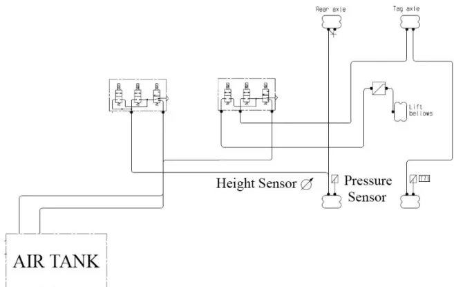
Analysing various configurations, it is evident that the pneumatic configurations can be broadly classified into two types, laterally connected i.e., the air springs on the left and right side of the same axle are connected to form one pneumatic circuit as illustrated in Figure 7. This type of pneumatic connection is predominant in trucks. Or they are longitudinally connected i.e., the air springs on drive and tag axles on the same side are connected to form a pneumatic circuit as illustrated in Figure 8. This type of pneumatic connection is predominant in buses. Observing the laterally connected pneumatic configurations, it is evident that there is one height sensor for the front axles and one for the rear axles irrespective of the number of axles on the front and rear and, there is a pressure sensor for each pneumatic circuit.

Figure 7 and Figure 8 depict the two broadly classified pneumatic configurations. 6x4B and 6x2A. Where the ‘6’ in 6x2A and 6x4B indicates the number of load-carrying wheels, the ‘2’ in 6x2A and ‘4’ in 6x4B indicate the number of driving wheels. The ‘B indicates front and rear air suspension, and the ‘A’ indicates front leaf suspension and rear air suspension which is illustrated in Figure 9.

11

Figure 8: 6x4B pneumatic configuration [Source: Scania]

Figure 9: 6x2 (top) and 6x4 (bottom) wheel configurations [Source: Scania]

Having identified the underlying common factors between the different pneumatic configurations, it is required to understand the working of the Electronic Level Control to efficiently develop the air suspension model.

12

2.4

Decoding the working of Electronic Level Control

The Electronic Level Control (ELC) is an important feature in Scania trucks. It is provided by a Supplier in the form of an Electronic Control Unit (ECU). The specifications required are provided by Scania and the supplier develops the corresponding hardware and software and this is installed in the trucks.

The primary function of the ELC is to control the air suspension. It has valves to fill and empty the air springs connected to the axles. pressure sensors to measure the pressure in the air springs. height sensors to estimate the ride height of the vehicle and for tag axles that are liftable, there is also a lifting air bellow.

The Electronic Level Control performs different functions which include [5]: • Level control - automatic and manual height adjustment

• Lifting and lowering tag axle - automatic and manually controlled • Traction help - adjusting load on driven axles for traction control

• Pressure ratio - adjusting load distribution between axles by pressure control • Kneeling - lowering for embarking or disembarking the vehicle

• Axle load - estimating weight of each axle on the road • Sidewalk detection

The code that is implemented in the ECU is supplier proprietary and is not shared to Scania. This makes understanding the working logic of ELC difficult. Therefore, an attempt must be made to understand its working through experimentation. However, very minimal information can be obtained by analysing a successful case of ELC. Thus, a specific scenario in which, due to specific load conditions the ELC has failed, is observed. A test vehicle named ‘Osaka’ and wheel configuration of 6x2/4 which has failed to achieve static equilibrium with respect to ride height and pressure is observed.

Figure 10 depicts the cyclic process of the Electronic Level Control trying to establish the static equilibrium by altering the pressure in the bellows and as a result altering the ride height of the vehicle. The two blue curves on the pressure curve indicate the upper and the lower limit of the tag axle. The red curve on the ride height and the pressure curve represents the drive axle and the green curve represents the tag axle.

13

Figure 10: Experimental results of failed ELC case [Source: Scania]

Initially, the tag axle is exhausted i.e., the air in the bellows is released using the valves. This reduces the pressure in the tag axle and the height of the tag axle reduces. However, since the height of the drive axle is also reduced due to tag axle exhausting and the air in the drive axle bellows are not released, the pressure in the drive axle increases. After that, the ride height and the pressure levels are checked, since the tag axle pressure is not within the limits, the next step in the process is carried out. The drive axle is now exhausted. This lowers the height of the drive axle and the tag axle, since the air in the bellows of tag axle is not exhausted, the pressure on the tag axle increases. Now, the pressure and the ride height are checked again. The pressure of the tag axle is within the limits; however, the ride height is below the target level. Hence the tag axle and the drive axle bellows are filled by letting air in through the valves, and the process is continuously repeated.

Observing this failed case, the basic principle behind the working of ELC can be understood and the variable that is utilised to manipulate the air springs is identified. Although the observed case is for one configuration, it can be expanded to other pneumatic and wheel configurations. However, this analysis of ELC cannot completely clarify the uncertainties with regards to pneumatic connections. This clarity can be achieved by analysing the current models and also through experimentation and physical testing on trucks.

14

2.5

Current air suspension models in ADAMS/Car

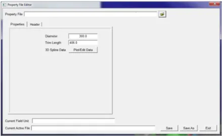
To develop a new air suspension model in ADAMS/Car, it is important to analyse the existing models for its strengths and limitations. There are two models available, the ‘air spring model’ and the ‘truck air spring model’ which is available in the ADAMS/Truck plugin. The ‘air spring’ model prominently used by Scania has air springs which utilizes preload as the control variable. In ADAMS, the preload is referred to as trim-load. Each air spring is associated with a property file (Figure 11). The property file has three parameters, the diameter of the spring, which is purely for graphical purposes; the trim length which is the design length of the air spring and 3D spline data. The 3D spline data determines the characteristics of the air spring as it is a plot between force (along the y-axis) and displacement (along the x-axis) with different trim loads along the z-axis. Trim-load is the value of the nominal force at given trim length and internal pressure of the air spring.

Figure 11: Property file editor of air spring

There are two modes available in this model of air spring: trim load and auto trim load as depicted in Figure 12. The trim load allows the user to manually choose a trim load that is to be applied on the spring throughout the simulation. During the simulations, the force in the air spring is calculated by interpolating the 3D spline data for the specific trim load curve using the AKIMA method.

In the auto trim load mode, the trim load applied on the truck is automatically chosen depending on the payload added to the truck. The calculation done to determine the trim load is with the help of subroutines of ADAMS solver and there is limited knowledge as to how the subroutines work.

15

In addition to this, a Scania specific plugin is used to adjust the trim load on different springs to achieve required axle weights (Figure 13). This plugin allows the user to specify the axle weights required, and using Scania proprietary code in ADAMS solver, the optimal payload required is calculated and this is added either to the payload, which is typical in many cases or to the axles with the help of dummy masses assigned to each axle, and the trim load is modified after changing the load on the axles to return the air spring to its design height. When the air spring reaches the design height and the modified axles weights are close to the required axle weights, the solver assumes successful static solution.

Figure 13: Axle weight set up using preload (Scania)

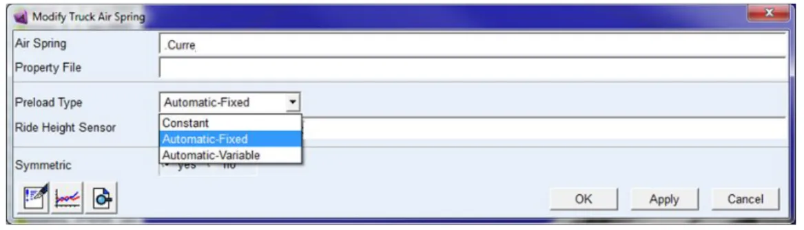
The second air spring model available is, ‘truck air springs’ which has same working and functionality as the normal air springs, but there are three modes for truck air springs as opposed to two modes. The three modes available are: Constant, Automatic-Fixed and, Automatic-Variable (Figure 14). The constant mode is similar to the ‘trim load’ mode of the ‘air spring model’, the trim-load is entered manually, and this is applied to the model throughout the simulation. In the automatic-fixed mode, the trim load is automatically adjusted during the initial static equilibrium solution and is kept constant thereafter. In the automatic-variable mode, the trim load is automatically adjusted continuously throughout the entire simulation.

Figure 14: Three modes of truck air springs model

Like the ‘air spring model’, the air springs in the ‘truck air spring’ model are also associated with a property file with the same three parameters, the difference between the two models arise in the working of automatic-fixed and automatic-variable modes. Both automatic modes require a ride height sensor to adjust the trim load during the simulation. A single ride height sensor is sufficient irrespective of the number of axles. The ride height sensor is a crucial

16

component as it calculates the ride height, which is the distance between frame and axle. When a deflection from the desired ride height arises, the ride height sensor identifies it in terms of angular change and calculates the required trim load to restore the air springs to desired ride height. This is done with the help of differential equations in ADAMS solver. The working of these differential equation will be discussed in detail in an upcoming chapter.

Both the air spring models available have the strength of automatically adjusting the trim load. However, there are more limitations to the models. In the air spring model that is currently utilized, the solution becomes statically indeterminate for trucks with 3 or more axles, i.e., the solver is incapable of determining an optimal trim load distribution among the air springs while maintaining the air springs at design height. Both models use trim load as the control variable to manipulate the forces in the springs, but do not provide any means for different air springs to communicate with each other. This could lead to air springs of the same circuit having different forces, thus causing unrealistic ride height and axle weights. Moreover, since there is no communication between the air springs, an Electronic Level Control cannot be implemented in both the models.

2.6

Identification of control variable

Many research papers which have been mentioned in Section 2.2.4 have developed and utilized force models i.e. used force as a control variable to manipulate the air springs and other components involved in the air suspension. Also, the available air spring models use preload force as a control variable to identify the forces acting in the spring. These can be considered as conventional approach since the multi-body dynamic models require force as an input. However, the goal of the thesis is to develop an air suspension model with Electronic Level Control that mimics the working of the actual ELC while maintaining the simplicity such that no external applications are required to provide accurate results. Analyzing the working of ELC, it is understood that pressure is used as the control variable and manipulation of force and ride height regulation is a consequence of the pressure control.

Therefore, in this thesis, pressure is chosen as the control variable to identify the optimal ride height and the required force input is calculated from the pressure.

17

3

Methodology and method

In this chapter, the different methods which can be implemented to achieve the goal of the thesis is laid out and the justification as to why the method is suitable or not suitable is explained. Also, a brief description of the chosen method is provided.

3.1

Methodology

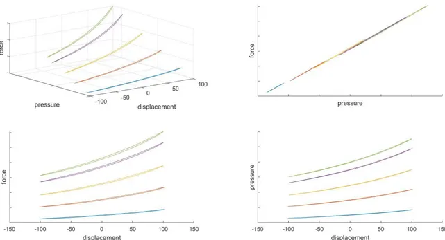
One method is to use the experimental results. The bellows are tested for adiabatic and isobaric conditions. For the adiabatic test, the air bellows is inflated to specific air pressure at design height. Then, the spring is given displacement and the corresponding forces are recorded while the valves are closed to prevent release of gas from the bellows. This is performed for different nominal pressures. For the isobaric test, the air pressure in the bellows are kept constant while altering the length or height of the spring. As discussed in earlier sections, the process that takes place in the air springs is closer to the adiabatic process. Hence the data from the adiabatic tests can be used to develop the model. Since the hysteresis is neglected some processing is required to represent the data without hysteresis. However, since the experiment is done for limited nominal pressures, accuracy of the result using this method depends on the interpolation capability of ADAMS solver which will be discussed in upcoming chapters. Another method which can be implement is by utilizing the force model developed by Leif Sortti [3]. The results from the model were compared with experimental results and the model was validated. The data from this model is produced without any hysteresis and furthermore, pressure curves at many different nominal pressures can be simulated using this method. However, this model was developed for a specific type of bellows and there is some manipulation required to produce the data required to build the model. Moreover, the results from this model were compared to the experimental data that is already available (Figure 15) to validate the model developed.

Thus, a better and simpler choice of method would be to use the experimental data for developing the air suspension model with pressure as the control variable.

The experimental data recording the pressure, displacement and force in the air spring at different initial air pressure is displayed in Figure 15. This data is then used as a 3D spline in ADAMS and also it is used to determine the relation between force and pressure of this specific air spring.

18

Figure 15: Experimental results of air bellows

3.2

Method of implementation

The air suspension model is implemented with help of a ride height sensor, which measures the deflection in terms of distance, instead of angular change like the present model. With this deflection value, the control variable, which is pressure in this thesis model, is identified with the help of differential equations in ADAMS solver. The identified value of the pressure indicates the nominal pressure which is the pressure value of the air spring when there is no deflection, and the truck is at ride height.

To identify the pressure in the air spring at every instant, the 3D spline data is referred. As mentioned, each air spring is referred to a property file which has a 3D spline data. In the present model, this 3D spline data is a plot of spring force and deflection at different trim loads which means the control variable is trim load. However, in the thesis model, the experimental data recording the pressure and displacement, at different nominal pressure of the air springs (Figure 16) will be used as 3D spline data in ADAMS.

19

Figure 16: Pressure vs Displacement at different nominal pressures

Using the AKIMA interpolation method, and with the identified nominal pressure value, the pressure vs deflection curve to be followed is chosen. And this curve is utilised as long as there is no change in the ride height and the payload. When there is a change, the optimal ‘pressure curve’ is identified again and that curve is followed. At every instant, the pressure in the air spring is calculated. With the determined pressure, the force in the spring is calculated by identifying the relation between the force and the pressure from the data from the experiment as displayed in Figure 15.

20

4

Physical testing

Physical testing on the truck is an important process which is required for various reasons. Primarily, before developing the model in ADAMS/Car there are several uncertainties which needs to be clarified through experimentation. These include the question, whether the bellows in the same circuit will have same pressure, even if the two bellows are loaded unevenly; Would the pressure distribution between two pneumatic circuits remain constant irrespective of the added payload. Moreover, to validate the developed model, experimental data is required to compare the results from the simulation.

To develop the model, initially it is beneficial to model for a configuration that is simple thus avoiding the complexities involved and it would be easier to verify the model. However, the choice of configuration must be made such that it can be applied to simpler or more complex configurations. The configuration choice also must consider the availability of the truck for testing. Taking these factors into account, the truck ‘Morgan’ which is depicted in Figure 17 is chosen and it has a configuration of 6x2A as shown in Figure 7.

Figure 17: Scania truck - Morgan

Before performing the tests, the objective for the test, the load cases, the parameters to be observed and the method of testing must be determined.

The objective is to observe and record the air spring variables while simulating different load case scenarios which represent the way payload might be added to the truck in real scenarios. There are five payload blocks and each of them weigh 1000 kg. Six different load cases are identified to represent different scenarios as depicted in Figure 18.

The parameters to be observed depends on the practicability and the available instruments required to record the parameters. Considering these factors, the following parameters are observed: the axle weights of the vehicle are measured using weight scales; the pressure in all four air bellows are measured using pressure sensors and the ride height of the drive axle on both left and right side is measured using draw wire distance sensors.

21

The method of testing is carried out in a way that, for each load case, there are six scenarios performed as shown in Figure 19. The six scenarios are that the truck is raised by 20 mm, 40 mm and up to full extension and then returned to the ride height level. Similarly, the truck is lowered by 20 mm, 40 mm and down to full compression and returned to ride height level. These six scenarios are performed primarily to ensure the repeatability of the air suspension system, i.e., to check whether the same pressure is attained after bringing the truck to its the ride height level from different ride heights.

Figure 18: Six different load cases performed in experimentation on truck.

Figure 19: Six different scenarios for each load case

The derived measurements are stored as arrays in MATLAB and the mean of the tag axle pressure is divided by the mean of the drive axle pressure to determine and verify the pressure distribution ratio of the truck obtained in experimentation with the truck configuration data. Similarly, the pressure value of all four bellows for six different load cases are found using the mean value. The values are tabulated as displayed in Table 1 and Table 2.

22

Table 1: Axle weight recorded for six case loads Axle Weight (tonnes)

Left Right Total

Case 1 Front Axle 3.82 3.56 7.38 Drive Axle 2.41 2.19 4.6 Tag Axle 1.53 1.38 2.91 Case 2 Front Axle 4.07 3.79 7.86 Drive Axle 2.24 2.05 4.29 Tag Axle 1.46 1.28 2.74 Case 3 Front Axle 2.84 2.6 5.44 Drive Axle 2.96 2.79 5.75 Tag Axle 1.93 1.76 3.69 Case 4 Front Axle 3.38 3.22 6.6 Drive Axle 2.39 2.69 5.08 Tag Axle 1.45 1.74 3.19 Case 5 Front Axle 3.5 3.14 6.64 Drive Axle 2.81 2.16 4.97 Tag Axle 1.95 1.32 3.27 Case 6 Front Axle 3 2.74 5.74 Drive Axle 1.39 1.23 2.62 Tag Axle 0.89 0.73 1.62

Table 2: Air Spring Pressure recorded for six different load cases Pressure (bar)

Left Right Mean

Case 1 Drive Axle 2.04 2.05 2.04 Tag Axle 1.39 1.19 1.29

Case 2 Drive Axle 1.81 1.82 1.81 Tag Axle 1.11 1.11 1.11

Case 3 Drive Axle 2.64 2.65 2.65 Tag Axle 1.63 1.64 1.63

Case 4 Drive Axle 2.22 2.23 2.23 Tag Axle 1.38 1.39 1.39

Case 5 Drive Axle 2.29 2.29 2.29 Tag Axle 1.35 1.36 1.36

Case 6 Drive Axle 0.69 0.70 0.70 Tag Axle 0.49 0.49 0.49

23

5

Implementation of air suspension model

There are different analysis modes in the ADAMS solver, however for the implementation of the air suspension model only two modes are of importance: Static and dynamic analysis mode.

5.1

Implementation of static model in ADAMS

The static mode of analysis is performed before the dynamic analysis and one of the purposes of this mode of analysis is to find a static equilibrium solution of the model. In the context of the thesis model, this means the ADAMS solver tries to perform the task of the Electronic Level Control, i.e., it identifies the balance between the pressure in the air springs and the desired ride height of the vehicle model.

To implement the static air suspension model in ADAMS solver, command batch script is used. In the command script, a ride height sensor is implemented and, a method to associate the deflection in ride height sensor with pressure is established. From the determined nominal pressure, the optimal pressure-displacement curve is determined. Thus, from the pressure, the force in the spring is identified.

To implement the ride height sensors in the command script, two markers are created, one on the frame of the vehicle and one on the drive axle. The distance between these two markers at any instant is the actual ride height. The distance between the frame of the vehicle and the drive axle without any deflection is the design ride height. Any deflection in the design ride height is considered as the displacement which is calculated by the difference between the design ride height and the immediate ride height calculated using the markers.

Through the identified difference in the ride height, the nominal pressure in the air springs is identified. This is accomplished with the help of differential equations declared as shown in Equation (5).

1000*(

_

_

_

_

)

y

=

design ride height actual ride height

−

The identified difference is multiplied by a factor of 1000 as it would allow for more precision control during small deflection of the vehicle.

To restrict the logic to work only for the static analysis mode, the differential equation is implemented with an ‘IF’ function of ADAMS solver. The ‘IF’ function with the attribute ‘MODE’ allows the equation to be applicable only during the static analysis mode and during the other analysis mode, the solution will be 0.

(

5 : 0,1000*(

_

_

_

_

), 0)

IF MODE

−

design ride height actual ride height

−

The number ‘5’ indicates the static analysis mode in ADAMS. The dynamic mode is represented by the integer ‘4’. However, initially only static model is implemented. The syntax of Equation (6) states if the solver mode integer is less than 5 or greater than 5, the solution is 0. But if the solver mode integer is equal to 5, then implement Equation (5).

24

The solution to the differential equation is accessed using the ‘DIF’ function. This function returns the integral of the differential equation. The ADAMS solver forces the solution of the integral to zero during the static analysis mode. However, when there is a deflection, the difference between the design ride height and actual ride height cannot be zero, hence it forces the constant of the integral solution to change until it satisfies the condition. The satisfied integral solution of the equation gives the nominal pressure in the air springs.

This value of the nominal pressure is for one pneumatic circuit. For this specific chosen test vehicle configuration, ‘Morgan’ this value is for the drive axle. For the pressure value in the tag axle, the tag axle to drive axle ratio according to the truck configuration data from Scania is used. In case of different pneumatic configuration, the respective vehicle configuration data can be used. Thus, there will be two different nominal pressures for two pneumatic circuits. With the identified nominal pressures, the pressure in the spring at every instant is calculated. This is accomplished using the experimental data of the characteristics of the air spring (Figure 16).

It is evident that the experiment is performed for a finite number of nominal pressure values and for each nominal pressure, the pressure in the air spring is recorded against the displacement of the air spring. However, if the identified nominal pressure value from the ADAMS solver happens to be of a value which is between two values from the experiment i.e., if the identified pressure value is 3.5 bar, there is no actual data recording the pressure in the air spring against its displacement with the initial value of 3.5 bar. In this circumstance, a method to interpolate the pressure-displacement curve is used, known as AKIMA interpolation method.

( , ,

)

AKISPL x z ID

In ADAMS solver, to utilize AKIMA interpolation, two independent variables, one along the x-axis (displacement) and the other one along the z-axis (nominal pressure) is required and it is referred to a 3D spline ID, which is the property file of the air spring. This forms the syntax for the AKIMA interpolation as indicated in Equation (7). AKIMA interpolation allows cubic interpolation in the y-direction and linear interpolation in the z-direction. Thus, the AKIMA interpolation helps in determining and interpolating the optimal pressure-displacement curve. However, the input to the spring in the multi-body dynamics model is a force input. To determine the force in the air spring, the experimental data is referred. The relation between force and pressure for this specific air bellow type is identified as linear from the data and Figure 15 (Top right); and then, a factor to convert the pressure into force is identified. This factor is multiplied with the pressure determined from the AKIMA interpolation based on the air spring’s displacement. Thus, the force in the air spring at every instant is identified which is further used as an input in the ADAMS model.

25

Thus, the syntax for identifying the force in the air springs using pressure as control variable can be written in the form of Equation (8)

0

* ( , / * 1, )

F=Ae AKISPL z h h P id (8)

F is the force in the air spring

Ae is the effective area of the air spring

h is the actual height of the air spring

h0 is the design height (trim length) of the air spring P1 is the control variable, the desired nominal pressure z=h-h0 is the displacement in the air spring height.

h/h0 is the factor used to modulate the nominal pressure (z-axis) to compensate for deviations from the design height.

In the context of the thesis model, the command script is written for the specific truck configuration. However, the purpose of the thesis model is that it should be adaptable to any truck configuration. Therefore, the command script is structured in a robust way such that only little modification is required to the script to adapt it for other pneumatic configurations. This essentially means the pressure and the force in each air spring is calculated individually and the relation between each spring is implemented through variables which are easily modified.

5.2

Implementation of dynamic model in ADAMS

The primary difference between the static and dynamic mode of the air suspension model is that, in the static model, the nominal pressure is calculated once, and the same value is used for the whole simulation but in dynamic model, the nominal pressure is calculated in the static analysis mode but it is allowed to vary throughout the simulation.

After identifying the optimal static solution, the ADAMS solver performs the dynamic simulation. It is the part of the simulation where the driving scenarios such as Single Lane Change, Step Steer etc., are performed on the vehicle model in ADAMS. If Equation (6) is used in the dynamic analysis mode, there would be no influence of ride height control as the solution or the integral of the equation is simply a constant. This may lead to results which are aberrant. To implement ride height control in the dynamic analysis mode Equation (6) has to be modified.

For implementing the dynamic model, two functions are utilized, SIGN and STEP function. In the SIGN function and the STEP function, the ride height error i.e., the difference between the design ride height and the actual ride height is used as the independent control variable. The ride height error is checked for its sign, i.e., whether it is positive or negative. The SIGN function has the syntax as shown in Equation (9). The value of ride height error is compared with zero, if the value is below zero, the output of the sign function will be -1, else it will be 1. This is significant as it helps in identifying what type of correction (positive or negative) is required to restore the ride height to the design value.

(1,

_

_

)

26

In reality, the ride height control is not activated immediately when the ride height deviates from the design value. A tolerance level is chosen until which no action is taken, this is called the dead-band value. It is used to reduce the wear on the valves and thus increase its lifespan. It is a variable that is chosen according to the manufacturer standards. It is usually given in both positive and negative range i.e., ± 8mm. To replicate the control logic, the dead-band is implemented in the dynamic model.

The logic of activating the ride height control after a tolerable limit is referred from S. X. Xing et al. [16] (Figure 20). It is implemented using the STEP function in ADAMS. However, since the SIGN function will be used in conjunction with the STEP function, the absolute value of the ride height error is sufficient to control both positive and negative errors. This also reduces the complexity of coding in ADAMS solver.

Figure 20: Ride height control activation range [16]

The syntax of the STEP function is shown in Equation (10). 0 0 1 1

( , , , , )

STEP x x j x j (10)

It requires an independent variable ‘x’; the value of ‘x’ where the step function begins, x0; the value of ‘x’ where the step function ends, ‘x1’; the initial value of the step function, ‘j0’, and the final value of the step, ‘j1’.

(

(

_

_

), 0.9*(

/ 2), 0, (

/ 2),1)

STEP abs ride height error

deadband

deadband

In context of the thesis model, the ride height error is the independent variable that the function applies to and, the step function begins when the ride height error value is 0.9 times the half of the dead-band value. This corresponds to the tolerable error range (Figure 20). The step function ends when the ride height error value is equal to the dead-band value, which refers to the limiting error. It signifies that the ride height control logic is dormant until the ride height error is 0.9 times the half dead-band value. And it remains active until the ride height error is returned to a value less than 0.9 times the half dead-band value.

The SIGN function multiplied with the STEP function is incorporated as the dynamic equation in Equation (6) to modify it as Equation (12).

( 5 : (1, _ _ )* ( ( _ _ ),0.9*( / 2),0,( / 2),1), 1000*( _ _ _ _ ),0)

IF MODE SIGN ride height error STEP abs ride height error deadband deadband

design ride height actual ride height

−

27

However, the dynamic model needs to be tested in ADAMS. This can be achieved in two ways. One way is to build a 3D road to simulate the conditions which affect the ride height of the vehicle and observe the results of the simulations. But this process is tedious and might require changes when testing with different scenarios. A far simpler method is to alter the desired ride height level as a variable with time in the command script. This is accomplished using the STEP function as shown in Equation (13).

( ,5.0, 480,5.2,520)

STEP time (13)

This is illustrated in Figure 21 where the desired ride height is 480 mm until time is 5 seconds and changes to 520 mm when time is 5.2 seconds. Thus, the step function is used to alter the design ride height.

A straight-line simulation. ‘maintain’ is performed on the ADAMS model of Morgan. Observing the results (Figure 21), it is evident that the actual ride height has overshoot, higher settling time and also has steady state error. These are three characteristics in the output that prove that a PID controller must be implemented to remove these deviations. An example of the errors in PID output is depicted in Figure 22. Moreover, the Electronic Level Control (ELC) is a controller, therefore in order to replicate the ELC it is required that a PID controller is implemented in the dynamic model.

28

Figure 22: Characteristics of the aberrant closed-loop step response.

5.2.1 Implementation of PID Controller

A Proportional Integral Derivate (PID) controller uses a control loop mechanism with feedback to continuously regulate process variables. A PID controller calculates the error between the measured output of the process variable and the desired set point and applies correction on the process variable using the proportional, integral, and derivative terms. A system or, a plant without any PID control resembles as depicted in Figure 23. There will be no method to correct any deviation occurring in the actual ride height as there is no feedback. This may lead to results as shown in Figure 21.

Figure 23: Vehicle model without PID control

A basic PID controller has a few key components. A plant, which is the vehicle model in the context of thesis; a desired set point (the desired ride height), a feedback loop for the measured process variable, and a PID control unit. The block diagram of the PID controller for this thesis model is depicted in Figure 24.

29

With the desired ride height set, the actual ride height from the feedback loop is compared with the setpoint (the desired ride height) and the error in the ride height is identified. The error is then fed to the PID control unit where the correction for the error is applied using the proportional, integral, and derivative terms. For the proportional term, the error is multiplied with the proportional gain (kp); for the integral term the error is integrated and then multiplied with the integral gain (ki), and for the derivative term, the error is differentiated with respect to time and multiplied with the derivative gain (kd). The gains values are specific to a controller and the plant; and they are identified with the help of tuning. The values from the proportional, integral, and derivative blocks are summed up and then it is fed to the vehicle model i.e., the ADAMS model which then again gives a ride height value which is fed as feedback. This loop helps in regulating the ride height value continuously.

The PID controller is implemented in ADAMS using differential equations. The identified error in the ride height is treated differently for the proportional, integral, and derivative blocks. For the proportional block, the ride height error which is stored as a variable is simply multiplied with the proportional gain (kp).

For the integral block, a differential equation with the ride height error as function is declared in explicit form i.e., it computes 𝑦̇ as shown in Equation (14). The solution to the differential equation i.e., the integral of ride height error is accessed using the DIF function and it is multiplied with the integral gain (ki).

( _ _ )

y= ride height error (14)

For the differential block, a differential equation with ride height error as function is declared in implicit form i.e., the ADAMS solver equates the expression to zero as shown in Equation (15). The solution to the differential equation, i.e., the time derivative of ride height error is accessed using the DIF1 function and it is multiplied with the differential gain (kd).

( _ _ ) 0

y− ride height error = (15)

The output from each block is then summed up and stored as a variable ‘PID output’. This variable is used in Equation (12) instead of the ride height error variable. Thus, the ADAMS vehicle model acts as the plant for the PID controller and the PID controller is implemented in the model. However, the output from the PID can have a lot of noise and to avoid this, generally a filter is implemented in the PID controller.

5.2.2 Implementation of low pass filter

With a PID controller, the output or, the measured signal might have small amplitude high frequency vibrations. These may seem trivial, however, since the PID has a pure derivative block, these trivial vibrations in the output can be amplified to values that lead to aberrant results. Thus, a filter to attenuate these high frequency noise must be implemented to the PID controller.

A low-pass filter is a filter that allows signals that are of a frequency lower than the cut-off frequency to pass and attenuates signals that are above the cut-off frequency. Cut-off frequency is a value that is chosen by the designer of the controller and it depends on the measured variable, the characteristic of PID controller and the frequencies that needs to be attenuated. It