Evaluation of view maintenance with complex joins in a data warehouse environment
(HS-IDA-MD-02-301)
Kjartan Asthorsson (kjarri@kjarri.net) Department of Computer Science
Högskolan i Skövde, Box 408 SE-54128 Skövde, SWEDEN
Final year project on the study programme in computer science 2002
Evaluation of view maintenance with complex joins in a data warehouse environment
Submitted by Kjartan Asthorsson to Högskolan Skövde as a dissertation for the degree of M.Sc., in the Department of Computer Science.
2002-06-14
I certify that all material in this dissertation which is not my own work has been identified and that no material is included for which a degree has previously been conferred on me.
Evaluation of view maintenance with complex joins in a data warehouse environment
Kjartan Asthorsson (kjarri@kjarri.net)
Abstract
Data warehouse maintenance and maintenance cost has been well studied in the literature. Integrating data sources, in a data warehouse environment, may often need data cleaning, transformation, or any other function applied to the data in order to integrate it. The impact on view maintenance, when data is integrated with other comparison operators than defined in theta join, has, however, not been closely looked at in previous studies.
In this study the impact of using a complex join in data warehouse environment is analyzed to measure how different maintenance strategies are affected when data needs to be integrated using other comparison operators than defined in a theta join. The analysis shows that maintenance cost is greatly increased when using complex joins since such joins often lack optimization techniques which are available when using a theta join. The study shows, among other things, that the join aware capability of sources is not of importance when performing complex joins, and incremental view maintenance is better approach than using recomputed view maintenance, when using complex joins. Strategies for maintaining data warehouses when data is integrated using a complex join are therefore different than when a theta join is used, and different maintenance strategies need to be applied.
Table of Contents
1 INTRODUCTION...1
1.1 Outline of the report ...1
2 DATA WAREHOUSING...3
2.1 Introduction to data warehouses ...3
2.2 Data warehouse definitions...4
2.3 Data warehouse architecture ...4
2.4 Data warehouse maintenance ...6
2.4.1 Maintenance Policies...8
2.4.2 Source capabilities... 10
2.4.3 Cost analysis and performance studies on view maintenance ... 10
3 JOINS...12
3.1 Types of join... 12
3.2 Algorithms for join operations ... 13
3.3 Complex join ... 14
4 PROBLEM DESCRIPTION...16
4.1 Aims and objectives ... 16
4.2 Expected results ... 16
5 METHOD...18
5.1 Identify a complex join ... 18
5.2 Analyze view maintenance with complex join ... 18
5.3 Compare different maintenance policies ... 18
5.3.1 Analytical modeling ... 19
5.3.2 Simulation... 19
5.3.3 Measurement... 19
5.3.4 Selecting the method ... 19
6 IDENTIFYING A COMPLEX JOIN...21
6.1 SWISS-PROT ... 21
6.2 PROSITE ... 23
6.4 Regular Expressions ... 25
6.4.1 Regular expressions in PROSITE ... 26
7 VIEW MAINTENANCE WITH A COMPLEX JOIN...28
7.1 Source capabilities ... 28
7.2 Integration of data with complex join... 29
7.3 Maintenance policies... 31
7.4 Summary of view maintenance with complex join ... 32
8 COMPARISON OF MAINTENANCE POLICIES...33
8.1 The evaluation framework... 33
8.1.1 Cost measurement ... 34
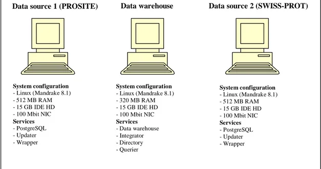
8.1.2 Architecture ... 34
8.2 Implementation ... 36
8.2.1 Modeling SWISS-PROT and PROSITE... 36
8.2.2 Modifying the framework to support SWISS-PROT and PROSITE ... 37
8.2.3 Validating the implementation ... 38
8.3 Experiments ... 38
8.4 Results ... 39
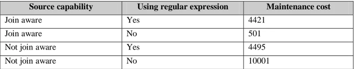
8.4.1 Join aware capability ... 40
8.4.2 Incremental vs. recomputed maintenance ... 41
8.4.3 Source size... 43 8.5 Summary... 45 9 CONCLUSIONS...47 9.1 Summary... 47 9.2 Discussion... 48 9.3 Future work ... 49 REFERENCES...51
APPENDIX A – SAMPLE DATA ENTRY FROM SWISS-PROT...54
APPENDIX B – SAMPLE DATA ENTRY FROM PROSITE...56
APPENDIX C – PROSITE AND SWISS-PROT TABLE DEFINITIONS...57
APPENDIX D – CONVERTING REGULAR EXPRESSION PATTERNS...60
APPENDIX F – SETTINGS FOR EXPERIMENT 2...64
Introduction
1
Introduction
Data warehouses are commonly used to load data from different data sources into a central repository, a data warehouse. This is done to offload the data sources, as well as being able to integrate data from different data sources. By integrating the data, it becomes possible to pose queries to the data warehouse which use data from multiple data sources.
Data warehousing has become a popular research topic in both business and computing. Building a data warehouse has shown to be a valuable investment for many organizations in today’s competitive business world (Connolly & Begg, 2002). Much research on how to maintain data warehouses, so the data warehouse gives a correct view of the underlying data sources, has been conducted. Several approaches, such as replicating the source databases at the data warehouse to ease the integration, or by letting the data warehouse query the sources to update the warehouse, have been taken in the data warehouse maintenance process.
Maintaining a data warehouse includes integrating data from different sources in order to build up a common view of the data. Sources in data warehouse environment are, by nature, autonomous and heterogeneous, which means that they are often not within the control of the data warehouse administrator and run on different platforms, using different technologies. Because of this, the integration of the sources can not always be done by using simple comparison operators, such as those defined by a theta join. Complex operators may be needed in order to integrate the sources. These operators may have different characteristics than the commonly used comparison operators (Zhou, Hull, King & Franchitti, 1995).
In this project the impact of using a complex join to integrate data in a data warehouse environment will be investigated. An example of a complex join will be identified and analysis will be conducted on how such joins will affect view maintenance by looking at the characteristics of the complex join. A close look will be taken at which join algorithms are available when using a complex join, and which limitations, if any, exist when performing such joins. Also, a comparison of view maintenance with a complex join and a theta join will be conducted in order to see in what aspects view maintenance with a complex join differs from the more simple value based joins.
1.1
Outline of the report
In chapter 2, a brief background information in the field of data warehousing and an overview of previous research in the field of data warehouse maintenance will be given. Different methods of maintaining data warehouses and how source capabilities can support the maintenance process will be discussed.
Chapter 3 describes how different data sets can be joined together to form a new data set. An overview of the most commonly used join types and algorithms in a traditional database environment will be given. The need to join two data sets by complex joins rather than a simple value based joins will also be discussed, since such joins are important in data warehouse environments.
In chapter 4 the problem under investigation in this project is described. The aim of the project will be defined and several objectives to reach the aim will be set. Finally a brief discussion of expected results will be given.
Introduction
Chapter 5 describes how the problem described in chapter 4 will be tackled. An overview of different methods to solve the problem will be given and one will be selected for this project.
In Chapter 6 to 8, a description of how the evaluation was conducted will be given. In chapter 6, the type of a complex join that is used in the project is presented. In chapter 7, an analysis on how a complex join may affect view maintenance, with focus on the join type identified in chapter 6, will be given. In chapter 8 a comparison between a complex join and simple value based joins will be made, in order to see in what aspects these differ.
Finally, in chapter 9, some conclusions will be drawn and suggestions for future work will be given.
Data Warehousing
2
Data Warehousing
In this chapter data warehouses are briefly explained and the rationale for using data warehouses discussed. Data warehouse architectures will be described with an overview of the most commonly used components in such architectures. Data warehouse maintenance will also be discussed and an introduction on current research in measuring the maintenance cost of data warehouses will be given.
2.1
Introduction to data warehouses
Data warehouses have gained much attention during the past years. Data warehouses are used to collect data from different information sources in an organization and to store it in a central repository (the data warehouse). Before data is loaded from a source to a data warehouse, it is often aggregated, transformed and cleaned in some way so it can be easily integrated with data from other sources (Connolly & Begg, 2002).
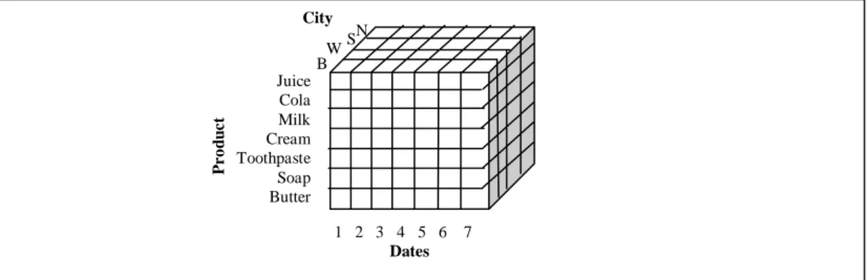
Data in data warehouses is usually modeled as multidimensional where each dimension represents some subject of interest. These dimensions are then joined together with so called fact tables (Connolly & Begg, 2002). An example of such dimensions may be a product, a city, and a date. These dimensions make it possible to see how much was sold of a product in a city during a certain day. This can also be aggregated, and a report for monthly sales of some product in given city can for example be created (Chaudhuri & Dayal, 1997). Figure 1 shows the structure of a multidimensional data.
Figure 1: Multidimensional data (adopted from Chaudhuri & Dayal, 1997). Each dimension of the cube represents some data dimension, building a three dimensional view of the data. By looking at the data from different dimensions, a different perspective on the data can be viewed and analyzed.
Dimensional modeling and data warehouse design is outside the scope of this dissertation, and no further details about how to model data in data warehouses will be given.
The advantages of building data warehouses to collect data from different information sources have attracted many businesses to build a data warehouse (Chaudhuri & Dayal, 1997). By building a data warehouse, it is possible to execute queries that join data from many different information sources. Summary reports are accordingly based on these queries. Data warehouses also make it possible to mine data to find hidden relations and discover new knowledge which may be useful for the organization (Connolly & Begg, 2002).
1 2 3 4 5 6 7 Dates Juice Cola Milk Cream Toothpaste Soap Butter P r o duc t N W B S City
Data Warehousing
The advantages of building data warehouse, mentioned above, have, among other factors, led to the development of data warehousing (Connolly & Begg, 2002).
2.2
Data warehouse definitions
In the literature, data warehouses have been defined in different ways. Chaudhuri and Dayal (1997, p. 65) define a data warehouse as “a collection of decision support
technologies, aimed at enabling the knowledge worker (executive, manager, and analyst) to make better and faster decisions”.
Connolly and Begg (2002, p. 1047) define a data warehouse as “subject-oriented,
integrated, time varying, non-volatile collection of data that is used primarily in organizational decision making”.
Quass, Gupta, Mumick and Widom (1996, p. 158) define the purpose of data warehouses as to “store materialized views in order to provide fast access to
integrated information”.
The definitions above focus on different aspects of data warehousing. The definition given by Chaudhuri and Dayal (1997) gives a very broad view of data warehousing and represents more the view of data warehouses from the information system engineering field, while Connolly and Begg (2002) and Quass et al. (1996) focus more on the database aspects of data warehouses.
For this project the database aspect of a data warehouse (e.g. maintenance of data warehouses) is of more importance than its function in an organizational context. The following definition of a data warehouse will be used for this project:
A data warehouse is a materialized view of data from one or more autonomous heterogeneous data sources.
It is important to note that the sources in data warehouse environments are autonomous which means that they are often not within the control of the data warehouse administrator. They may be external websites or databases that are outside the organizational boundaries of the data warehouse. By heterogeneous it is meant that the data sources can be run on different platforms, using different technologies. A data source may be an HTML document on a website, an XML based database, a relational database, a legacy system etc.
2.3
Data warehouse architecture
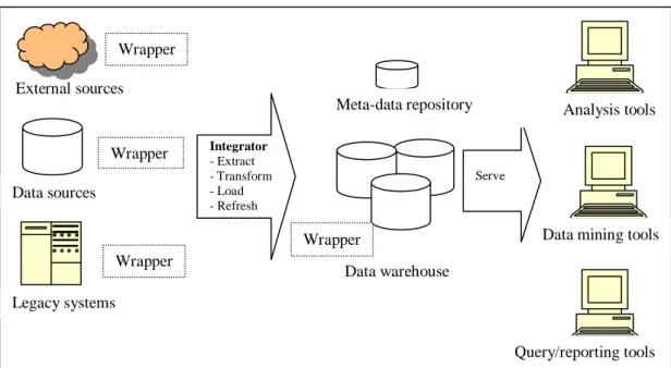
A data warehouse architecture consists of different elements that interact with each other. A brief overview of some common elements in a data warehouse architecture will be given below.
• Data sources. Data sources supply data to the warehouse. This can be old
legacy systems in the organization, various databases, web pages or even external data sources such as publicly available databases outside the organization (Connolly & Begg, 2002). The data warehouse is built around these data sources, where each source supplies data to the data warehouse for one or more of its dimensions.
• Wrappers. Wrappers are optional elements in the architecture and are used to
emulate some capability of the data sources in the data warehouse environment. The sources may need to report changes that have occurred in
Data Warehousing
the source from one time point to another. If the source can not provide this functionality, it may be possible to use wrappers to emulate this behavior so the source would seem to offer this functionality. Depending on the situation, the wrapper can be located either on the data source side or on the data warehouse side. If the source is not within control of the data warehouse administrator, it may be impossible to place the wrapper on the source side, and the only possibility would be to place it in the data warehouse. If the wrapper is located on the data source side it will increase the load on the source since the wrapper will take both CPU and memory from the source host. If the wrapper is located on the data warehouse side it will, in many cases, increase the network load between the data warehouse and the data source since more data needs to be transferred between them (Engström, Gelati & Lings, 2001).
• Integrator. The integrator is responsible for integrating, extracting,
transforming, aggregating and cleaning the data, before it is stored into the data warehouse. This is important in order to successfully integrate the data from different data sources and store it in the data warehouse. An example of such a transformation could be converting the data from e.g. kilometers to meters in order to have the data from all sources stored in same units in the data warehouse (Connolly & Begg, 2002).
• Data warehouse. The data warehouse holds the integrated data. This could be
a standard RDBMS or any other type of database system. The data warehouse often contains, as mentioned earlier, summarized data. The data in the data warehouse is also often time varying. This means that one dimension of the data is time (e.g. summary of daily sales are stored in the data warehouse). The database system used for the data warehouse thus needs to have support for the type of queries that are usually executed on such data. This often requires some extensions to the standard query language SQL (Chaudhuri & Dayal, 1997).
• Meta repository. The meta repository stores information about the warehouse
schema and where data is stored. It can map the view of the data sources to the view in the data warehouse. It is also useful for the query manager of the data warehouse to help build execution plan (Connolly & Begg, 2002).
• Tools. The data warehouse can have different tools. This includes tools to
perform various analyses on the data in the warehouse, tools to make reports from the data in the warehouse and tools that can be used to mine the data in order to discover new knowledge from the data in the warehouse (Connolly & Begg, 2002).
Data Warehousing
Figure 2: Data warehouse architecture (Adopted from Chaudhuri et al., 1997)
In this project a focus will be made on the data sources and how the data is propagated to the integrator and integrated. The process of propagating the data from the sources to the data warehouse is often called data warehouse maintenance and will be discussed in next section.
2.4
Data warehouse maintenance
Data warehouses store copies of data from other databases. This is also said to be a
materialized view of the source data. That is, the data warehouse contains a copy of
some parts of the source databases which can be seen as a new view of the source data.
A view can be either virtual or materialized. A virtual view is a view which is constructed for a data set with the help of a query language while a materialized view is constructed by creating a new physical data set for the view (Blakeley, Larson & Tompa, 1986). Accessing a materialized view is usually faster than accessing a virtual view because a virtual view needs to be recomputed each time it is accessed while a materialized view is a copy of the source data, stored physically on a disk. A materialized view is therefore especially useful if the view is queried frequently (Gupta & Mumick, 1995).
Since a materialized view is a copy of the base data set, it introduces the problem of keeping the view consistent with the base data set. Keeping the materialized view consistent with the source databases may in some applications be important, while other applications do not require the view to be constantly consistent with the data sources. The process of keeping the materialized view consistent with the data sources is called view maintenance. Different approaches exist for maintaining materialized views in data warehouses. One approach is to replicate the sources in the data warehouse and create so called auxiliary views (Quass et al., 1996). This means that all the data in the source that is needed in order to build the materialized view in the data warehouse will be replicated in the data warehouse as well. This implies that when the view in the data warehouse needs to be updated, no queries to the sources will be needed since all the needed data will replicated in the auxiliary views (Quass
Data sources External sources Integrator - Extract - Transform - Load - Refresh Data warehouse Legacy systems Serve Meta-data repository Query/reporting tools Data mining tools
Analysis tools
Wrapper Wrapper
Wrapper Wrapper
Data Warehousing
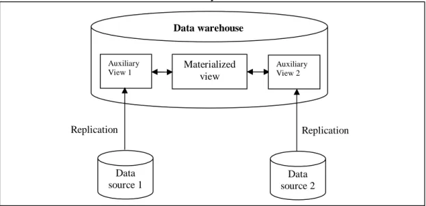
et al., 1996). These kinds of views are also called self-maintainable views (Quass et al., 1996; Wang, Gruenwald & Zhu, 2000). Figure 3 illustrates how a typical architecture for such view maintenance may look like.
Figure 3: Data warehouse architecture with self-maintainable view. Data source 1 and 2 are replicated in the data warehouse as auxiliary view 1 and 2. The materialized view updates itself by querying the auxiliary views.
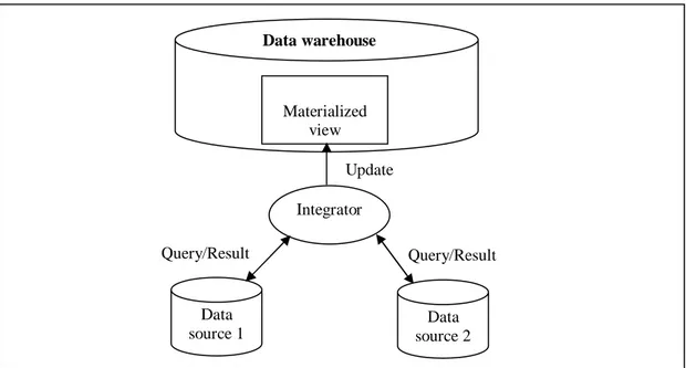
Another approach for doing view maintenance is not to replicate the sources in the data warehouse. This means that whenever the materialized view in the data warehouse needs to be updated, the data warehouse may need to send queries the other sources to successfully update the view (Quass et al., 1996). Such views are sometimes called non self-maintainable views (Wang et al., 2000). When using non self-maintainable views in a warehouse environment the sources need to be queried in order to update the view. This also means that if a source sends a change notification to the data warehouse, the warehouse may need to send queries to other sources as well in order to successfully update the view. In cases where parts of the sources go offline, the view maintenance may get blocked since the warehouse may need to send queries to the sources that are offline (Wang et al., 2000).
Figure 4 illustrates the architecture of a non self maintainable view. Materialized view Data warehouse Auxiliary View 1 Data source 1 Replication Replication Auxiliary View 2 Data source 2
Data Warehousing
Figure 4: Data warehouse architecture with non self-maintainable view. The integrator sends queries to the sources in order to update the data warehouse.
The problem of maintaining materialized views has been well studied in the literature (Blakeley et al., 1986; Gupta & Mumick, 1995; Hull & Zhou, 1996). Many of the earlier studies only considered centralized environments for the view maintenance, which is not directly applicable to data warehouse maintenance where sources are often autonomous and heterogeneous (Zhuge, Garcia-Molina, Hammer & Widom, 1995). In the early studies it is often assumed that sources have “knowledge” of the materialized view and can provide delta changes (changes that have occurred in the source from given time point) to the materialized view. This can not be assumed in data warehouse environments where sources are often outside the control of the data warehouse administrator (Zhuge et al., 1995).
Maintaining data warehouses where sources are heterogeneous and autonomous requires new studies on maintenance algorithms that can handle sources with such different characteristics. This has been addressed in more recent studies on data warehouse maintenance (Zhuge et al., 1995; Gupta, Jagadish & Mumick, 1996).
2.4.1 Maintenance Policies
Several methods for view maintenance that describe how and when the view maintenance should be executed have been developed. Gupta and Mumick (1995) discuss two methods for view maintenance. The maintenance can either be done
incrementally or by recomputing the view.
Recomputing the view means that for each update in the data sources the view needs to be regenerated. This operation is expensive and creates a lot of overhead on both the sources and the materialized view since the source needs to send all the data to the data warehouse each time the warehouse needs to be updated. It is, however, a simple solution to keep the materialized views up-to-date (Gupta & Mumick, 1995).
Incremental maintenance is performed by calculating what parts of the changes in the source affects the view and updating the view accordingly. This approach is more complicated than recomputing the view from scratch, but increases performance in most situations (unless the change in the source is very large) (Gupta & Mumick,
Materialized view Data warehouse Data source 1 Integrator Query/Result Update Query/Result Data source 2
Data Warehousing
1995).
Several research projects have been conducted on incremental view maintenance and some algorithms have been developed. Zhuge et al., (1995) discuss anomalies in data warehouse maintenance. They describe how data warehouse maintenance differs from the traditional materialized view maintenance because of the heterogeneous and autonomous nature of data warehouses. They also show how a data warehouse view can get into an incorrect state when the data warehouse is doing a view update at the same time as the data in the sources is changing. To solve this problem they propose the Eager Compensating Algorithm for view maintenance. The Eager Compensating Algorithm is based on traditional incremental view maintenance algorithms, but uses extra compensating queries to avoid that the data warehouse gets into an incorrect state.
Three policies for deciding when view maintenance should be executed have been discussed in the literature (Hanson, 1987; Zhuge et al., 1995). These policies are:
• Immediate view maintenance
• Periodic view maintenance
• Deferred (on demand) view maintenance
Depending on the situation, one of these maintenance policies is selected for the data warehouse maintenance. Which policy to select depends on the requirements that are set on the view in the data warehouse, but such requirements may differ between different applications.
Immediate view maintenance
An immediate maintenance policy updates the materialized view after each update in the source (Hanson, 1987). This means that when source is updated, the change is propagated to the materialized view immediately. Immediate view maintenance is applicable in systems where the view has a high query rate and it is important that the view is always consistent with the sources. It is, however, not a feasible option in situations where the sources are updated frequently since there is an overhead associated with each update as the change needs to be propagated to the materialized view (Colby, Kawaguchi, Lieuwen, Mumick & Ross, 1997).
Periodic view maintenance
A periodic maintenance policy updates the materialized views periodically. This can leave the materialized view in an inconsistent state compared to the sources, so applications reading from materialized view when using a periodic policy must be able to tolerate stale data (Colby et al., 1997).
Deferred (on demand) view maintenance
A deferred maintenance policy updates the materialized views on demand (Hanson, 1987). This results in slower queries on the materialized view since the view has to update itself from the sources as needed. It also increases the update performance on the sources since the changes in the sources are not propagated to the materialized view until the materialized view is used (Colby et al., 1997).
Data Warehousing
2.4.2 Source capabilities
Sources in a data warehouse environment can have different capabilities which can be used in the view maintenance process. Source capabilities can be classified according to their impact on maintenance. Engström, Chakravarthy, and Lings (2000) make the following classification of the capabilities offered by sources:
• View aware. View aware means that the source has the capability to return
data for a specific view in a single query. If this capability is missing, the source returns all data entries to the data warehouse since it has no query capability to return only the data that is of use for the data warehouse.
• Delta aware. Delta aware means that the source has the capability to return
changes that have occurred in the source from given time point. This capability is especially useful when the data warehouse is incrementally updated since it returns only the changes which make incremental updates in the data warehouse simpler.
• Change active. Change active means that the source has the capability to
notify an external application (e.g. the data warehouse) that changes have occurred. This is required for immediate view maintenance so the data warehouse can be updated immediately when changes occur in the source.
• Change aware. Change aware means that the source has the capability to
deliver the time of last modification to the source.
It is further noted that if a source can not provide these capabilities they can be emulated with the help of wrappers. A wrapper is a software that is installed either on the source or on the data warehouse which emulates the desired source capabilities (Engström et al., 2001).
2.4.3 Cost analysis and performance studies on view maintenance
There are a number of factors that influence the maintenance cost of a data warehouse and several studies have been conducted to analyze what factors influence the view maintenance.
Wang et al. (2000) studied self-maintainable and non self-maintainable views by measuring how many rows were accessed in the warehouse as well as the storage space usage. In brief, their study shows that using self-maintainable views frees the sources from all maintenance activities since the relevant part of the sources are replicated at the data warehouse. This has the clear disadvantage that more space is needed at the data warehouse side to store the replicated data. Using a non self-maintainable view does, however, not require extra space at the data warehouse side, and no algorithms needs to be developed for the replication mechanism. View maintenance using non self-maintainable views also slows down the sources since the sources need to process extra queries when updating the view. Unavailable sources will also block the view maintenance which is considered bad for obvious reasons. Colby et al., (1997) investigated how to support views with multiple maintenance policies, that is, maintaining many views, which may have different maintenance policies. Colby et al. (1997) claim that their study is important since the different maintenance policies are very different in performance and data consistency. Their studies shows among other things that immediate maintenance penalizes update
Data Warehousing
transactions, while deferred maintenance penalizes read transactions. Further the study shows that when more than 10-20% of the base data set changes recomputation of the view is a better approach than to incrementally update it.
Engström et al. (2001) investigated how source capabilities influence maintenance overhead and quality of service, and for this purpose they developed a data warehouse framework. The framework allows adjustments to be made to different parameters in the data warehouse environment. Using the framework it becomes therefore possible to analyze the impact of those parameters on the data warehouse maintenance process. The parameters that are configurable are: source capabilities, location of wrapper, and maintenance policy (incremental, recomputed, immediate, deferred, and periodic). The framework measures different things such as:
• Staleness. Measures how up-to-date the data in the view is, compared to the sources.
• Response time. How long time it takes when a query is executed on the data warehouse until the results are displayed.
• Integrated cost. The cost for all data processing in the sources and the warehouse and the communication delay.
Additional measurement is also performed, measuring things like total execution time, number of updates, size of updates, time spent performing updates etc. This can be useful to help detecting possible errors in the experiments and to gain more insight into exactly what is going on in the experiment (Engström et al., 2001).
The study by Engström et al. (2001) presents some initial experiments using the framework. First experiments show that source capabilities are very important factor in the data warehouse maintenance process and needs to be carefully considered when designing data warehouse applications.
Joins
3
Joins
Combining two data sets has been well studied in set theory and the following set operators have been defined (Elmasri & Navathe, 2000): union, intersection,
difference and the Cartesian product.
To illustrate the set operators consider the sets R and S.
• The union of R and S, denoted byR∪S, includes all elements from either R or S or both R and S. No duplicates are included (Elmasri & Navathe, 2000).
• The intersection of R and S, denoted byR∩S, includes all elements that are in both R and S (Elmasri & Navathe, 2000).
• The difference between R and S, denoted byR−S, is defined as all elements that are in R, but not in S (Elmasri & Navathe, 2000).
• The Cartesian product of R and S, denoted byR×S, is defined as the concatenation of every element in R with every element in S (Connolly & Begg, 2002).
A join operation can be seen as a subset of the Cartesian product since join is really a selection of the Cartesian product, using the join predicate as the selection formula (Mishra & Eich, 1992). Join is a common operation in databases since often there is no need to concatenate all elements in one set with all elements in the other. By using the join operators it is possible to combine two data sets, using a condition, to only get a subset of the Cartesian product (Connolly & Begg, 2002).
How to join two data sets has been well studied in the relational database research. This knowledge can even be extended when not working with relational databases since the join types and principles are not only applicable to relational databases. In a data warehouse environment, just as in relational database environments, sources need to be joined together. Unlike relational databases the joins often need to be done on attributes that do not have the same data types, or can not be matched with simple matching operators (Zhou, et al., 1995). This creates some differences in the availability of join techniques since such joins have quite different characteristics than joins that use simpler join operators.
In this chapter an overview of what join types are commonly used will be given and what characterizes these. Different implementations of join algorithms will also be discussed, but performing join is one of the most costly operations in relational databases (Connolly & Begg, 2002). Finally, joins in a data warehouse environment will be discussed and contrasted with joins in a traditional database environment.
3.1
Types of join
Different types of joins that have been defined, which are applicable in different situations (Connolly & Begg, 2002). The most commonly used types of joins are presented below.
• Theta join. A theta join is a join that is performed on two relations with any of
the following comparison operators: <, <=, >, >=, =, !=.
Joins
is equality. This implies that the resulting relation will include two identical values.
• Natural join. A natural join is an equijoin, but without duplication of common
attributes.
• Outer join. When using any of the joins named above and where a tuple in one
relation does not match any in the other relation the tuple will not be included in the resulting relation. An outer join, however, includes even those tuples that have no matching attributes in the other relations.
• Semijoin. A semijoin is a special kind of join that allows two relations to be
joined, but the resulting relation will only include attributes from one of the joining relations. This technique is quite common when dealing with distributed databases where queries are joining data from two distributed databases. This can help in reducing the network traffic and therefore speed up performance (Elmasri & Navathe, 2000).
3.2
Algorithms for join operations
Different methods have been developed to perform the join operations described above. Several algorithms have evolved through the years and the most common ones today are the following (Connolly & Begg, 2002):
• Nested loop join
• Sort-merge join
• Hash join
These algorithms differ in cost applying them and are suited for different situations. The nested loop join is the simplest join algorithm and joins the relations by processing them tuple by tuple at time. The relations are defined as outer and inner relations. For each tuple in the outer relation all tuples in the inner relations are scanned and matching tuples are placed in the output relation (Mishra & Eich, 1992). This algorithm is quite inefficient since it requires multiple scans of the inner relation. Another variant of nested loop join is indexed nested loop join which is similar to the traditional nested loop join, but uses indexes if possible. That means that if the inner relation has an index on the joining attribute it is possible to spare the full scan of the inner relation by looking up the matching tuples in the index instead (Connolly & Begg, 2002).
Sort-merge join is used when both relations being joined are, or can be, sorted on the joining attribute. The algorithm begins by sorting both relations on the joining attribute (if not sorted already). Then the relations are merged together by scanning through them. The merge operation is quite efficient since the relations are sorted and it is not needed to scan the relations more than one time (Mishra & Eich, 1992).
The hash join algorithm can be used for natural or equijoins and exploits a hash function to join the relations. The hash join algorithm hashes the joining attribute in one relation and builds a hash table that maps the joining attribute to tuples. The joining element in the other relation is then hashed and checked if it matches any value built in the hash table. If it matches then the tuples are joined and placed in the output relation (Mishra & Eich, 1992).
Joins
Other variants of hash join have been developed such as hash-partitioned join which is built on the ideas to divide-and-conquer. The problem of joining the relation is partitioned into several sub-problems which can be more easily solved (Mishra & Eich, 1992).
Little discussion has been made in the literature about joins that are based on more complex operators instead of the standard theta join operators. Most databases only support the standard set of operators for joining two data sets and do not allow joins to be done with custom made operators. Two databases have been identified that allow custom operators to be created and used in joining data sets, these are Oracle and PostgreSQL1. The capability to create custom defined operators are important for complex join types, since by using this capability the comparison between two elements can be based on an arbitrary function.
3.3
Complex join
Different join types have been presented and a brief discussion of what join algorithms have been developed has been given. In some instances, however, joins need to be performed with more complex operators than defined in theta joins. For the purpose of this project such joins will be defined as a complex join.
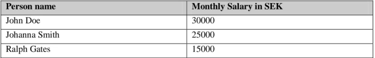
Complex joins are based on functions that need to be applied to the joining attributes to be able to match them. To demonstrate this, a simple example will be given of a join between two data sets where one of the data sets includes salary information for persons and the other data set contains different tax classes2. These data sets are illustrated in Table 1 and Table 2 below.
Person name Monthly Salary in SEK
John Doe 30000
Johanna Smith 25000
Ralph Gates 15000
Table 1: Employee salaries
Tax class Tax percent Year salary in SEK
Normal 30 100000 - 200000
High 45 200000 - infinite
Table 2: Tax classes
To join the data sets to find out what tax class an employee is a part of, the monthly salary attribute in the employee data set, and the yearly salary in the tax classes’ data set needs to be joined together. It is, however, not possible to simply compare these fields. First the salary in the employee database needs to be multiplied with 12 in order to find the yearly salary for the employee. A special operator is also needed to compare the yearly salary of the employee with the yearly salary range data type in
1
However no survey of database servers has been done to investigate which ones do support custom defined operators.
2
This is a simplified example and could possibly be solved using SQL. The point is however that not all joins are done by the comparison operators defined in theta join. In many cases a function needs to be applied to the data in order to join it.
Joins
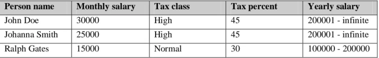
the tax classes’ data set. To join these two data sets is therefore not possible with the standard comparison operators offered by a theta join and needs special treatment. The resulting data set, when the data in Table 1 and Table 2 is joined, is presented in Table 3 below.
Person name Monthly salary Tax class Tax percent Yearly salary
John Doe 30000 High 45 200001 - infinite
Johanna Smith 25000 High 45 200001 - infinite
Ralph Gates 15000 Normal 30 100000 - 200000
Table 3: Employee and tax classes data sets combined
Although this example is simple, it clearly demonstrates that a join between different data sets can not always be performed directly with the operators in theta joins.
The usage of complex comparison operators is quite common in object oriented programming languages where it is allowed to define custom operators. The same need is in data warehouse environment, where data sets need to be compared based on a custom defined operator that can have arbitrary complexity.
Using complex join in data warehouse environment does raise several questions related to the view maintenance. For one, the sources may not have the capability of performing the complex join, which requires an alternative solution such as using wrappers to emulate the source capability or to perform all joins in the integrator. The usage of optimization techniques such as indexes may be limited, and the availability of join algorithms may be less than when using the theta join operators.
The join function may also be computationally complex and take long time to execute. This may affect the staleness of the data in the warehouse since immediate maintenance may be delayed and recomputed maintenance may therefore be an infeasible option in many cases.
Problem description
4
Problem description
Maintenance of materialized views has been well investigated in many studies (Blakeley et al., 1986; Gupta & Mumick, 1995; Hull & Zhou, 1996). Many studies have also been conducted on how different maintenance policies can affect the cost of maintaining the materialized views (Colby et al., 1997; Engström et al., 2001; Wang et al., 2000; Zhuge et al., 1995).
However, no study seems to have focused on how maintenance of materialized views is affected when sources need to be joined by a complex join instead of the traditional comparison operators as defined in a theta join.
Joining data sources with more complex operators is especially important in data warehouse environment where data comes from independent autonomous heterogeneous sources which may store the data in different formats. In such cases it is often needed to apply a function on the data to be able to match it (Zhou et al., 1995). As have been previously discussed, such join operators may have quite different characteristics than the theta join operators. Issues like what join algorithms and optimization techniques are available to perform such joins needs to be considered. It is also unclear how such joins affect the view maintenance when compared with a theta join.
It is therefore of interest in this project to investigate what implications it has on view maintenance when a materialized view is based on sources that need to be integrated with a complex join.
4.1
Aims and objectives
The aim of his project is to evaluate how view maintenance is affected when sources are integrated with a complex join instead of a simple value based theta joins in data warehouse environment.
To reach the aim of the project several objectives have been set up.
• Identify a complex join to use in the evaluation. This complex join will be used during the evaluation to analyze how it affects the view maintenance.
• Analyze maintenance policies for materialized views based on complex joins. This analysis is conducted to get a better understanding of the impact complex join has on the view maintenance and what maintenance strategies can be used when integrating data sources with a complex join.
• Compare the maintenance strategies for a complex join with view maintenance based on a theta join and see in what aspects these differ. This is important in order to be able to compare the results of this work with previous studies on view maintenance when sources have not been joined with a complex join.
4.2
Expected results
The aim of this project is to evaluate the impact of using complex join in a data warehouse environment and explore how using a complex join affects the maintenance of the data warehouse. Hopefully this work will contribute to the field of data warehouse maintenance by showing how view maintenance is affected when sources needs to be integrated by a complex join. It is believed that view maintenance
Problem description
with a complex join, will have quite different characteristics than view maintenance with a theta join and the purpose of this project is to explore some of the differences. Further it is hoped that this project will give ideas about what join algorithms can be used when dealing with complex join and what problems and limitations exist when performing such joins.
Method
5
Method
In this chapter different methods will be presented for solving each of the objectives set for this project. For each objective the different methods for solving it will be discussed and the most appropriate method will be selected.
5.1
Identify a complex join
Identifying a complex join is crucial for this project. The complex join needs to demonstrate a common problem in the field of data integration when a function needs to be applied on data in order to join it. It is considered important that the complex join that will be used in the evaluation represent some common type of complex join that is a problem in real life, rather than some obscure made up join.
Identifying a complex join in a data warehouse environment can be done in several ways. A literature study can be done in the field of data warehousing with focus on data integration or even case studies describing the usage of data warehouses. This should give an overview of what kind of data integrations are being done in the field of data warehousing and possibly give several examples of cases where the data integration needs to be done with a complex join.
Another way is to conduct a survey of public databases available on the Internet. By looking at different public databases it may be possible to identify different databases that contain data that is in some way related to each other. If related databases are identified it may be possible to join the data from the different databases in order to get a new view on the data. This join may possibly require a complex join since the data may have different characteristics.
In the present study a search will be done on the Internet for databases that could be used to demonstrate a complex join. It should be possible to integrate the databases using complex join, and the databases should be used in some application domain.
5.2
Analyze view maintenance with complex join
To understand the impact of maintaining views based on a complex join it is important to know what maintenance policies are available and how they may be affected when sources need to be integrated with a complex join. It is also important to investigate how sources can be joined effectively when using a complex join instead of a theta join.
To achieve this, a literature study will be conducted in the field of maintaining materialized views in order to gain insight into current research and possibly find any leads to how maintenance of materialized view with a complex join may be performed. A literature study will also be done to learn about different join algorithms. An analysis of the join algorithms will be done, in order to get an understanding for how they can possibly be used when joining data sets with a complex join.
5.3
Compare different maintenance policies
Many of the properties, that are interesting for this evaluation of maintenance policies using complex joins, are performance related. Properties such as comparing the execution time for the integration using different settings, measuring the network load
Method
etc. are of interest. Several methods exist for doing such evaluations. Jain (1991) identifies three different methods for doing performance evaluation; analytical modeling, simulation and measurement.
In this section each method will be discussed briefly and related to this project in order to learn which approach is most suitable.
5.3.1 Analytical modeling
Analytical modeling is used to model the system under evaluation and then use formal methods for proving its correctness. Performing such modeling requires many assumptions to be made about the real system and good knowledge of the system. Analytical modeling is, however, often considered to have limited credibility since the number of assumptions is often high and often it does not match the reality. It is also very difficult to get a good understanding of the system being modeled, and there is a risk that some aspects in the model are incorrect (Jain, 1991).
5.3.2 Simulation
Simulation is used in situations where it is hard, or impossible, to use a real implementation of the system. By using a simulation, the target system, and environment is modeled in the simulator and executed. This, however, is a complicated task because the simulation needs to give a correct representation of the real system and environment to be useful (Jain, 1991). It is also difficult to decide the level of detail in the simulation, that is, how closely should the simulation reflect the real system?
Compared to analytical modeling, simulation requires fewer assumptions to be made about the system and the environment. It is, however, a time consuming task and error prone process since it is hard to know that the simulator gives a correct view of the reality.
5.3.3 Measurement
Measurement is used to measure the performance of a real system in operation. This may involve collecting statistics of network load, number of queries, execution time of queries etc.
It is important that the system is measured under normal circumstances and normal workload. Doing experiments on the system under some special circumstances may not give correct measures of the system (Jain, 1991).
5.3.4 Selecting the method
Choosing a method for the evaluation is not a trivial task. Using analytical modeling is, as mentioned earlier, a complex task that needs a good understanding of the system. It also requires several assumptions to be made about the system behavior which often results in much simplification of the system (Jain, 1991). Based on the fact that analytical modeling is proven to require much simplification of the system and many assumptions to be made it is ruled out as a possible option for this project. The goal for the evaluation in this project is to show a practical evaluation of how maintenance is affected when using complex joins.
Method
does, however, not exist and building one will require a lot of work. Since the time is limited for this project, building a simulator is not an option and is therefore ruled out as a possibility.
Applying the measurement technique, to measure the performance of a real system, may be feasible option. Doing a measurement using a real system should give a good indication on how maintenance of materialized views is affected when joining data with a complex join. Such measurement may involve collecting statistics for the integration cost when maintaining the data warehouse.
For this study a measurement of a prototype implementation of a data warehouse has been selected as a method to compare the view maintenance with a complex join against view maintenance with a theta join. This may be seen as a middle step between simulation and a real system. The prototype should offer basic data warehouse functionality, and allow a measurement of different properties in the maintenance process such as integration cost etc. While this approach does not measure a real data warehouse, it should give indication for how maintenance of a real data warehouse will be affected when integrating sources with a complex join.
Identifying a complex join
6
Identifying a complex join
In this project a complex join is defined as a join based on other join operators than defined in a theta join. This definition applies to different kinds of joins using different operators. For this work it is important to identify an example of a complex join that could be seen as representative for other complex joins.
A search has been made on the Internet for databases suited for this project. The requirements on the databases are that the databases should be used in real life and it should be possible to integrate the databases with a complex join. Two publicly available databases were identified that fulfill these requirements. The databases are SWISS-PROT3, which stores information about protein sequences, and PROSITE4, which stores information about protein families. The protein sequences in SWISS-PROT are defined by a sequence of characters that represent the amino acids5 in the protein. The protein families in PROSITE are defined by a regular expression pattern. A regular expression pattern is a string which describes properties of another string. In order to join the databases to see which protein sequences match which protein families, a regular expression function needs to be applied.
SWISS-PROT and PROSITE are widely used by researchers in the field of bioinformatics (Attwood & Parry-Smith, 1999) and using these databases in a data warehouse scenario may be seen as a realistic application, and a good example of a complex join. Regular expressions are also used in many other application domains than bioinformatics such as by authors, web indexing machines, and other areas. In this chapter, an overview of these two databases and a discussion of their characteristics and usage will be given. After this, regular expressions will be discussed and explained how regular expressions are used in these databases by giving a detailed example of how the regular expression patterns are used in PROSITE.
6.1
SWISS-PROT
The development of the SWISS-PROT database began in 1986 by a joint effort of the Department of Medical Biochemistry of the University of Geneva and the European Molecular Biology Laboratory (EMBL) (Attwood & Parry-Smith, 1999). At a later stage the Swiss Institute of Bioinformatics (SIB) joined the effort and today the database is maintained by EMBL and SIB (Attwood & Parry-Smith, 1999).
SWISS-PROT contains protein sequence entries with citation details and taxonomic data (descriptions of the biological source of the protein). Additionally, the protein sequences are annotated with information such as the function of the protein, and other information that are believed to be of interest (Bairoch & Apweiler, 2000). The main design principles behind SWISS-PROT are to offer annotation to the data, minimize redundancy in the data and to be easily integrated with other databases. By offering annotation on the entries in the database the data is more helpful for the users. The annotation includes a wide variety of information that is considered useful for the user. Minimizing redundancy means that each protein sequence only has one 3 Available at http://www.expasy.ch/sprot/ 4 Available at http://www.expasy.ch/prosite/ 5
Identifying a complex join
entry in the database. It is quite common in other protein sequence databases that each protein sequence may have several entries in the database. This happens when there is a conflict about the sequence, e.g. if different research reports have given different information about the sequence. In SWISS-PROT this conflict is solved by noting this different information within the single sequence entry. It is also considered important that the database should be easily integrated with other databases. This has been solved in SWISS-PROT by adding so called pointers to the sequence entry which can refer to entries in other databases (Bairoch & Apweiler, 2000).
The SWISS-PROT database has become one of the most popular protein databases in the world and is widely used by researchers, both in commercial and educational environments. One of the reasons for its popularity is the easy navigational format of the database as well as the quality of the annotation in the database (Attwood & Parry-Smith, 1999).
The data
The data in the SWISS-PROT database is available in several text documents that are structured in a well-documented format. Each entry starts with an identification tag (ID) for the entry and ends with an end tag (//). Between these tags there can be many tags describing the different properties of the protein sequence entry. For this project only a subset of the available data in the database is of interest.
A sample data entry for SWISS-PROT is listed in appendix A. The entry contains a lot of information, but interesting parts for this project have been marked specially. These fields are:
• Entry name (ID)
• Primary accession number (AC)
• Cross-references (to PROSITE) (DR)
• Sequence information (SQ)
The entry name describes the identification of the entry.
ID 143B_HUMAN STANDARD; PRT; 245 AA.
Example 1: Entry name from the SWISS-PROT database
In this example the entry name describes a human protein, which has 245 amino acids. The entry name is, however, not unique and can change between releases of the database. In order to provide a static identifier the primary accession number (AC) was introduced.
AC P31946;
Example 2: Access number from the SWISS-PROT database
In this case the access number is P31946 and uniquely identifies this protein sequence entry, even between database releases.
The cross reference in SWISS-PROT is used to link the entry to other entries in external databases such as PROSITE, EMBL and others.
DR EMBL; X57346; CAA40621.1; -. DR EMBL; AL008725; CAA15497.1; -. DR EMBL; BC001359; AAH01359.1; -.
Identifying a complex join DR HSSP; P29312; 1A38. DR MIM; 601289; -. DR InterPro; IPR000308; 14-3-3. DR Pfam; PF00244; 14-3-3; 1. DR PRINTS; PR00305; 1433ZETA. DR ProDom; PD000600; 14-3-3; 1. DR SMART; SM00101; 14_3_3; 1. DR PROSITE; PS00796; 1433_1; 1. DR PROSITE; PS00797; 1433_2; 1.
Example 3: Cross reference entry in the SWISS-PROT database
Example 3 shows the cross references for our example protein sequence entry. In this case there are 12 cross references defined, one in each DR line. As can be seen in the example there are references to EMBL, PROSITE, Pfam and several other databases. For this project the PROSITE references are of importance.
The sequence information field contains the actual sequence data for the protein entry.
SQ SEQUENCE 245 AA; 27951 MW; 0BCA59BF97595485 CRC64; TMDKSELVQK AKLAEQAERY DDMAAAMKAV TEQGHELSNE ERNLLSVAYK NVVGARRSSW RVISSIEQKT ERNEKKQQMG KEYREKIEAE LQDICNDVLE LLDKYLIPNA TQPESKVFYL KMKGDYFRYL SEVASGDNKQ TTVSNSQQAY QEAFEISKKE MQPTHPIRLG LALNFSVFYY EILNSPEKAC SLAKTAFDEA IAELDTLNEE SYKDSTLIMQ LLRDNLTLWT SENQGDEGDA GEGEN
Example 4: Sequence entry in the SWISS-PROT database
The first line in the sequence field is header information which shows how many amino acids the sequence has, molecular weight and a checksum for the string. The sequence header line is followed by the sequence data, which is stored in one or more lines.
6.2
PROSITE
PROSITE is also maintained by the Department of Medical Biochemistry of the University of Geneva and the European Molecular Biology Laboratory. PROSITE contains sequence patterns for protein families. The patterns are regular expressions that describe properties of the sequence string that is part of that protein family. Using this information it is possible to categorize unknown protein sequences into known protein families (Falquet, Pagni, Bucher, Hulo, Sgrist, Hofmann & Bairoch, 2002). Not all protein families can be defined with a string pattern. In some cases the sequences that belong to certain protein family are too different to form a common string pattern. In these cases other methods need to be applied in order to calculate which sequences belong to which protein group. These techniques include the use of
profiles. A profile is a table of position specific amino acid weights and gap costs
(Falquet et al., 2002). In this dissertation the profile based entries will not be used, and will not be discussed further.
The PROSITE database has been developed with some leading concepts such as
completeness, which means that the database should contain as many as possible
patterns and profiles. It should have high specificity which means that it will detect most correct sequences and not many incorrect ones. Another goal with PROSITE is to keep up-to-date documentation which should be reviewed periodically. Last, but not least, the database should have strong relationship with the SWISS-PROT database (Falquet et al., 2002).
Identifying a complex join
The data
The data in PROSITE is kept in text files and is like SWISS-PROT, tagged in each line with special marker. The data starts with and ID tag which includes the identification of the entry and ends with an end tag (//). A sample data entry for PROSITE is listed in Appendix B.
There is a lot of information stored in each PROSITE entry, but for this project only a subset of it is of interest. The following information will be used in this project:
• The identification string (ID)
• The access number (AC)
• The pattern (PA)
• Cross references (DR)
The identification tag is used to identify the entry and describe the type of the entry. Possible entry types are PATTERN, MATRIX and RULE.
ID 1433_1; PATTERN.
Example 5: An identification line from the PROSITE database
The example above shows PROSITE entry with ID 1433_1 and is of type PATTERN which means that the protein group this entry represents is defined by a regular expression pattern. The other types, MATRIX and RULE, are other ways of defining the family, but these are not of interest for this project since only regular expression matching will be used.
The access number (AC) is another field used to identify an entry in the PROSITE database. Unlike the identification field the access number does not change from one release of PROSITE to another. It is therefore advised to use the access number to identify entries in the database. Below is an example of such entry.
AC PS00796;
Example 6: An example PROSITE access number entry
In these cases when the protein family is defined by a regular expression pattern, the pattern field is used. An example of such entry is given below.
PA R-N-L-[LIV]-S-[VG]-[GA]-Y-[KN]-N-[IVA].
Example 7: An example PROSITE pattern entry
The pattern entry in PROSITE is a regular expression pattern which describes the properties of the sequences that belong to this protein family. A more detailed explanation on how to read the regular expression patterns will be given in section 6.4.1.
Links to SWISS-PROT are given in the cross references field by listing the access number of the SWISS-PROT entries that match the given PROSITE entry. Not only does the link include the SWISS-PROT entries, but also information about the correctness of the classification, that is if the given SWISS-PROT entry is correctly classified by the pattern or not.
DR Q91896, 143Z_XENLA, T; P29311, BMH1_YEAST, T; P34730, BMH2_YEAST, T;
Identifying a complex join
DR P42656, RA24_SCHPO, T; P42657, RA25_SCHPO, T; DR P29306, 143X_MAIZE, P;
DR P93211, 1436_LYCES, N;
Example 8: An example PROSITE cross reference entry
As seen in the example above, several references can be in each DR line. Along with the access number in the SWISS-PROT database the entries include the entry name and information about if the entry was correctly classified by the pattern or not.
6.3
Using SWISS-PROT and PROSITE together
As have been shown, the two databases, SWISS-PROT and PROSITE, are closely linked together through the data reference field. However, these are not necessary in order to join the two databases together since it is possible to use the regular expression pattern (in these cases the PROSITE entry is based on a regular expression pattern) to join the two data sets.
Joining the databases together by using the regular expression pattern requires the sequence patterns in SWISS-PROT to be matched against the regular expression patterns in PROSITE. Such operation needs a regular expression matching engine to perform the comparison which will be discussed in the next section.
The two different ways of joining PROSITE and SWISS-PROT together are ideal for the evaluation in this project. By using these databases, it is possible to explore the differences in the view maintenance, when using the data from the reference fields to join the databases, and when using the regular expression pattern to join the databases.
6.4
Regular Expressions
The patterns in PROSITE, which are used to define the protein families, are based on regular expressions. A regular expression is a mechanism to match string patterns in text. Navarro and Raffinot, (1999, p.198) define a regular expression as:
A regular expression is a generalized pattern composed of (i) basic strings, (ii) union, concatenation and Kleene closure of other regular expressions.
The Kleene closure is defined by the "*" operator used in regular expressions, to specify a match for zero or more occurrences of the preceding expression (Aho, Sethi & Ullman, 1986). For example, the regular expression "re*gular" would match the string "rgular", "regular", "reegular", "reeegular", and so on.
Regular expressions are supported by many programming languages that are commonly used for text manipulation such as Perl, Python, AWK (Friedl, 1997). Many algorithms have been developed to search for regular expressions in text. One of the first algorithms (Friedl, 1997) developed for searching regular expressions was made by Ken Thompson in 1968. In his article he describes how the algorithm was implemented in a form of a compiler for the IBM 7094 computer (Thompson, 1968). Many other algorithms have been developed since then, many of them are implemented in well known UNIX tools such as grep (agrep, egrep, gnu grep etc.) which are text search tools which use regular expressions to search text documents (Friedl, 1997).
Identifying a complex join
Besides being an important part of the PROSITE database, regular expressions are useful in other different application domains. Other areas that use regular expressions are for example system administrators, which use regular expressions to examine different log files and other text extraction tasks. Authors also use regular expressions frequently to do various text lookups and replacements (Friedl, 1997; Navarro & Raffinot, 1999). Lately, regular expressions have also become important when querying semi-structured data such as XML documents. Such expressions are called regular path expressions and open the possibility to navigate through XML document based on path expressions, which can be defined with regular expression patterns (Milo & Suciu, 1997).
6.4.1 Regular expressions in PROSITE
There exist many different notations for expressing regular expressions. Even though these differ in syntax, the concept is always the same and they are built on the same foundation (Fredl, 1997). In PROSITE regular expressions are built with the following semantic (Bairoch, 2001):
• Each element is represented with the IUPAC one letter codes that represent the amino acids in the sequence.
• To represent any amino acid the letter ‘x’ is used.
• To represent a list of possible entries a ‘[]’ are used around the entries. An example is [ALT] which stands for A or L or T.
• Opposite to the ‘[]’ meta characters, the ‘{}’ are used to list entries that do not match. An example is {ALT} which means all characters other than A, L or T.
• To separate elements a slash ‘-‘ is used.
• Repetition of an element can be done by using parenthesis. An example of how repetition can be used is ‘A(3)’, which will match the string ‘AAA’.
• When a pattern is restricted to either the start or the end of a sequence the symbols ‘<’ and ‘>’ are used in the beginning and in the ending of the sequence respectively.
• A period ends the pattern.
To further illustrate how the regular expressions work in PROSITE a few examples will be given below, and a detailed explanation on how to interpret the pattern.
[AC]-x-V-x(4)-{ED}.
Example 9: Regular expression (adopted from Bairoch, 2001)
The first part of the pattern, [AC], means that the sequence can start with either an A or C. Next pattern is x, which means that any character is allowed. There after, a V is required in the sequence. The x(4) part of the pattern means that the next four characters can be of any type. The last part of the pattern {ED} means that all characters are valid except E and D. In brief, the pattern can be translated as: [A or
C]-any-V-any-any-any-any-{any but E and D}. <A-x-[ST](2)-x(0,1)-V.
Identifying a complex join
The first part of the pattern in Example 10, <A, means that the pattern must match the beginning of the sequence and that the first character is A. The next part of the pattern
[ST](2), means that either the character S or T is valid, two times in a row.
x(0,1) means that next character in the sequence can be any character or none. The
final part of the pattern, V, means that only the character V is valid. To summarize, following translation can be given: A-any-[S or T]-[S or T]-(any or