Research Institute of Industrial Economics P.O. Box 55665 SE-102 15 Stockholm, Sweden
info@ifn.se
IFN Working Paper No. 1377, 2021
The Comparative Impact of Cash Transfers and a
Psychotherapy Program on Psychological and
Economic Well-being
Johannes Haushofer, Robert Mudida and Jeremy
Shapiro
The Comparative Impact of Cash Transfers and a
Psychotherapy Program on Psychological and
Economic Well-being
∗
Johannes Haushofer
†Robert Mudida
‡Jeremy Shapiro
§January 4, 2021
Abstract
We study the economic and psychological effects of a USD 1076 PPP unconditional cash transfer, a five-week psychotherapy program, and the combination of both inter-ventions among 5,756 individuals in rural Kenya. One year after the interinter-ventions, cash transfer recipients had higher consumption, asset holdings, and revenue, as well as higher levels of psychological well-being than control households. In contrast, the psychotherapy program had no measurable effects on either psychological or economic outcomes, both for individuals with poor mental health at baseline and others. The effects of the combined treatment are similar to those of the cash transfer alone. JEL codes: C93, O12, D90
∗We thank the participants for their time; Tilman Graff, Magdalena Larreboure, Esther Owelle, and
Michala Riis-Vestergaard for excellent research assistance; the staff of the Busara Center for Behavioral Economics; and the staff of the NGO delivering the intervention, for fruitful collaboration and
com-ments. We thank Victoria Baranov, Barbara Biasi, Chris Blattman, Michelle Craske, Julian Jamison,
Crick Lund, Joanna Maselko, Petra Moser, Robert Östling, Miranda Wolpert, and seminar and confer-ence participants at the World Bank, BREAD, St. Andrews, LSE, Tilburg, Michigan, University of Penn-sylvania, University of Connecticut, Northeastern University, UCLA, and Bocconi, for comments. This study was funded by grants to Jeremy Shapiro by the Gates Foundation and an Anonymous Donor, and by Princeton University. Johannes Haushofer is grateful for financial support from Jan Wallanders och Tom Hedelius stiftelse. IRB approval was obtained from Princeton University (protocol no. 7375) and the Kenya Medical Research Institute (Non-KEMRI protocol no. 531). The study was pre-registered at https://www.socialscienceregistry.org/trials/3928.
†Stockholm University, NBER, BREAD, Busara Center for Behavioral Economics, MPI for Collective
Goods, and Research Institute of Industrial Economics. johannes.haushofer@ne.su.se
‡Strathmore Business School. rmudida@strathmore.edu
Recent work in economics and psychology has suggested that poverty and low psychological well-being may mutually reinforce each other (Ridley et al.
2020; Lund et al. 2011). For example, poverty may lead to stress, which
over time can cause mental illness (Hammen 2005; Haushofer and Fehr 2014). Conversely, poor mental health may affect labor market participation and pro-ductivity, and thus may exacerbate poverty (Schoenbaum et al. 2002; Biasi, Dahl, and Moser 2019; Ravensteijn and Schachar 2018). This potential feed-back loop suggests that interventions that alleviate poverty may be effective in both reducing poverty and improving mental health. Conversely, interven-tions that target mental health may improve both mental health itself, and poverty. In addition, if mental health and poverty are strong complements, interventions that address both poverty and mental health may be particularly effective in improving both outcomes.
Here we compare the individual and joint impact of an unconditional cash transfer and a psychotherapy program on measures of both economic and psy-chological well-being. We randomly assigned 5,756 low-income households in rural Kenya to one of four treatment conditions. 540 households in 60 villages received an unconditional cash transfer of USD 1,076 PPP (USD 485
nomi-nal; “CT”).1 525 households in 60 different villages were treated with Problem
Management Plus (“PM+”), a mental health intervention delivered by trained community health workers (CHWs). This program was developed specifically for low-resource settings by the World Health Organization (WHO), and is generally considered a flagship psychotherapy intervention for these contexts. Importantly, it has previously been shown to be effective in improving
men-tal health in Kenya (Bryant et al. 2017).2 A third group of 493 households
in another 53 villages received both cash transfers and PM+ (“CT&PM+”). Comparing outcomes of these groups with a pure control group of 1703 house-holds in another group of 60 villages allows us to determine the causal impact of
1The PPP rate for Kenya at the time of the study was 46.49. The transfer corresponds
to about 20 months of per capita control group consumption.
2Bryant et al. (2017) report a 0.57 standard deviation (SD) improvement in the General
Health Questionnaire (GHQ-12) among women who had been exposed to gender-based vio-lence 3 months after they participated in the program as part of a randomized experiment.
these interventions. In villages receiving the CT-only and PM+-only interven-tions, we also surveyed 1,237 and 1,219 non-recipient households, respectively, allowing us to estimate spillover effects of these interventions at the village level. In CT&PM+ villages and CT villages, we randomly allocated half of cash transfer recipients to receiving a lump sum transfer, and the other half a sequence of 5 weekly transfers, to study the impact of transfer frequency.
We administered a detailed survey both before the interventions, and about a year after they ended. The cash transfer was effective in improving both psy-chological and economic well-being: we find a 20 percent increase in monthly consumption in cash transfer recipients relative to the control group about a year after the intervention; a 47 percent increase in asset holdings; and a 26 percent increase in household revenue. An index of psychological well-being increases by 0.23 standard deviations (SD), and scores on the GHQ-12 men-tal health questionnaire—a widely used screening instrument for psychiatric morbidity—improve by 0.16 standard deviations. In contrast, the PM+ in-tervention affects neither economic nor psychological outcomes after one year: consumption and asset holdings both increase by 5 percent, and revenue by 9 percent, but these effects are not statistically significant. Similarly, the psy-chological well-being index is not affected by the PM+ treatment, showing a non-significant effect of −0.01 SD. The components of the index, such as psychological distress, happiness, and life satisfaction, also show no treatment
effect.3 Importantly, the PM+ treatment also has no effects on psychological
well-being or mental health amongst those participants who had high psy-chological distress at baseline. We also find no evidence that PM+ has early positive effects that dissipate quickly over time: even those participants who received the program most recently relative to the endline survey (about 7 months prior) show no improvement in psychological well-being at endline.
Outcomes in the group that received both the cash transfer and the PM+ intervention are similar to those in the group that received only the cash
3We observe a 0.24 SD increase in intimate partner violence (IPV) reports among female
PM+ recipients, but this effect is not significant after adjusting for multiple comparisons, and is not observed in more alternative measures of IPV that minimize response bias.
treatment: asset holdings increase by 41 percent, revenue by 17 percent, and psychological well-being by 0.27 SD. Consumption shows a somewhat smaller treatment effect than in the cash-only group, with a non-significant 7 percent increase, but the 95 percent confidence interval includes increases up to 18
percent. Weekly cash transfers are somewhat more effective in improving
economic outcomes compared to lump-sum transfers, and have similar impacts as lump-sum transfers on psychological well-being. We find little evidence of spillovers of either intervention to non-recipient households.
Thus, our main finding is that after one year, cash transfers have larger effects on economic and psychological well-being than the PM+ mental health intervention, which itself produces no improvements relative to control. Impor-tantly, the per-household cost of the cash transfers was lower than that of the PM+ intervention. The PM+ intervention is therefore both more expensive
and less effective in affecting our outcomes of interest.4
What explains the negligible impacts of PM+, even on outcomes which it specifically targets, such as psychological well-being? First, we were powered to detect PM+ treatment effects of 0.17 SD on psychological well-being. This compares favorably to typical effect sizes of psychotherapy on psychological outcomes, which are around 0.6–0.7 SD in the literature as a whole (Cuijpers et al. 2010; Cuijpers et al. 2013), 0.49 SD across low- and middle income countries (Singla et al. 2017), and 0.57 SD in a previous study of PM+ in Kenya (Bryant et al. 2017). Thus, lack of power is unlikely to explain our findings. To further confirm this claim, we use an approach based on Bayesian statistics which is not commonly employed in field experiments, but which can provide useful information. We ask: What is the probability that the observed null effect of PM+ reflects a true underlying null effect? This probability is given by the negative predictive value (NPV), defined as the share of null observations that reflect true null effects, rather than false negatives. We show that even with a 90 percent prior in favor of its effectiveness, the post-study
4If only marginal costs of the PM+ program are considered, i.e. per-session payments
to the CHWs without any administrative costs, the PM+ intervention may be more cost-effective for some outcomes if the positive but non-significant point estimates of PM+ are taken seriously.
probability that PM+ produces effects larger than 0.40 SD in our setting is only 10 percent.
Second, we largely rule out experimenter demand effects (i.e. a desire by participants to give responses that conform to the expectations of the survey-ors), using an approach proposed by De Quidt, Haushofer, and Roth (2018): when we present participants with explicit hypotheses about what we expect them to respond to self-report questions about depression, their responses do not change measurably relative to when they do not receive this information, suggesting that demand effects do not play an important role in our self-report measures. Note also that in our setting, demand effects would be likely to in-crease rather than reduce observe treatment effects.
Third, notice that the success of the PM+ intervention in a previous study in Kenya (Bryant et al. 2017) limits the explanatory power of several other explanations. Bryant et al. (2017) delivered PM+ to urban women who had experienced gender-based violence, and found improvements in psychological distress 3 months later. Importantly, the short (5 week) duration of the pro-gram; its content; and the fact that it is delivered by laypeople were the same in this previous study, arguing against these variables as explanations for our null effect. In addition, the implementation of the program in our study was done by the same NGO as in this previous study in Kenya. Thus, implemen-tation differences are unlikely to explain the lack of impact.
The previous study differed in four ways from the present one: it was con-ducted in an urban rather than a rural setting; impacts were measured after 3 months rather than 1 year; it was delivered to women who had experienced gender-based violence, rather than a general population sample; and it em-ployed 23 CHWs to deliver PM+ to 209 participants, while the present study employed 72 CHWs to deliver PM+ to 1018 participants, possibly resulting
in a loss of fidelity due to scale.5 We find it unlikely that the urban setting
accounts for the positive effects in the earlier study. As mentioned above, the
5In a trial of a layperson-delivered psychotherapy for perinatal depression in South
Africa, Lund et al. (2020) attribute their null results to a combination of lack of fidelity of intervention delivery and lack of competence of non-specialist, inexperienced CHW counsel-lors.
delay between intervention and endline is also unlikely to explain our null re-sults, as we observe no detectable effects even for participants who received the
intervention 7 months prior.6 Heterogeneity analysis in our study shows that
PM+ has no effects even for female participants, and for female participants who experienced high levels of intimate partner violence. Finally, we consider it unlikely that the intervention was low-fidelity in our setting, because the same NGO used the same extensive training and supervision protocols they had developed during the previous study.
A possible remaining explanation is that the program in the previous study, even though it was nominally the same as in our study, was delivered with the explicit goal of addressing gender-based violence. It is conceivable that the same program may be more effective when it is deployed to solve a specific problem. This mechanism would also explain the large positive effects of a similar program after seven years found by Baranov et al. (2020): this program was geared to alleviate post-partum depression. Similarly, Ghosal et al. (2016) find an increase in savings and health behavior 15 months after a self-esteem training for sex workers in India. Here, too, the stigma associated with sex work provided a clear target for the intervention. Thus, a likely explanation for the lack of lasting PM+ impacts in this study, despite successes in other studies, is that the program was delivered as a general-purpose intervention without a pre-defined problem to address.
It should be noted that the programs studied by Baranov et al. (2020) and Ghosal et al. (2016) were also more intensive, with 16 and 8 sessions, respectively, compared to 5 in PM+. Intensity alone is unlikely to explain our null effects, because the five sessions of the PM+ program did produce short-term effects in Bryant et al. (2017). But intensity may combine with circumscribed intervention goals to produce lasting effects. Thus, the most successful interventions may be those that are high-intensity and have specific goals.
6It remains possible that the PM+ program had positive effects after 3 months, but that
they had dissipated after 7 months. However, this would have to be a very steep decline, which we find somewhat implausible.
This explanation is also consistent with the results of several other recent studies which find positive effects of psychological interventions on psycholog-ical and economic outcomes: they either target more circumscribed problems, or, when they do not, are either more intensive or measure impacts over a shorter time horizon. For example, McKelway (2020) shows that a nine-session self-efficacy training in India increases women’s labor market participation four months later; Bernard et al. (2014) find that a single “aspirations” video in-creases human capital investment in Ethiopia after six months; and Haushofer, John, and Orkin (2019) show that two short trainings aimed at time prefer-ences and executive function in Kenya increase drinking water chlorination 3 months later.
A caveat to this explanation is the closely related study by Blattman, Jami-son, and Sheridan (2017), who use a similar design as ours to study the effects of a USD 200 cash transfer and a psychotherapy intervention in Liberia, both alone and in combination. At short time horizons (several weeks), they find im-pacts of both interventions on economic and psychological outcomes, including depression and distress. At a time horizon of one year, neither of the individ-ual treatments has effects on economic outcomes or depression and distress, although the combined treatment does. These findings are similar to ours in that we also find that the psychotherapy program has limited effectiveness af-ter one year. However, the psychotherapy inaf-tervention in Blattman, Jamison, and Sheridan (2017) was much more intensive than ours, with 3 weekly ses-sions over 8 weeks; and it aimed to address a specific problem, namely crime and violence. This study therefore suggests that an even intensive intervention that targets a specific problem may not be sufficient on its own to generate
lasting psychological and economic effects.7 It therefore remains an open
ques-tion precisely how program intensity and specificity combine to create lasting impacts.
Our study also contributes to literatures in economics and psychology that
7The fact that Blattman, Jamison, and Sheridan (2017) find little impact of the cash
transfer after one year may result from the smaller magnitude of the transfers, or differences in study population and context.
study the effect of cash transfers on economic and psychological well-being. In particular, a number of studies have shown that unconditional cash trans-fers improve both economic and psychological outcomes in developing coun-tries, such as Blattman et al. (2016) in Uganda and Baird, De Hoop, and
Özler (2013) in Malawi.8 More generally, economic interventions such as
as-set transfer and ultra-poor graduation programs often have positive impacts on both economic and psychological outcomes (Bandiera et al. 2017; Baner-jee et al. 2015; Bedoya et al. 2019). Our study confirms these results, and suggests that the impact of cash transfers is rather robust across studies and settings. In fact, with a few exceptions, the impacts of cash transfers on both economic and psychological outcomes in this study are remarkably similar to those we reported previously for a similar program in a different region in Kenya (Haushofer and Shapiro 2016). Even within the present study, the effects of the cash-only treatment arm and the combined cash and PM+ treat-ment are remarkably similar across most outcomes. Cash therefore appears to be a robust intervention that reliably improves economic and psychological well-being.
The remainder of this paper is structured as follows. Section I describes the design and methods of the study. Section II summarizes the analytic approach. Section III presents results. Section IV concludes.
I.
Design and methods
The design and methods were specified in a pre-analysis plan available at https://www.socialscienceregistry.org/trials/3928 (Haushofer, Riis-Vestergaard, and Shapiro 2019). An overview of the design is shown in Figure 1, and details on timing are given in Online Appendix Table A.1.
I.A
Village selection and village randomization
The study was conducted in partnership with the a large international NGO in Nakuru County in Central Kenya. Nakuru County was selected due to high levels of poverty, high baseline rates of poor mental health (at baseline, 33 percent of our sample were classified as suffering from psychological distress; see Section II.C), and because the NGO already had established an infrastruc-ture there. They provided a list of villages in the region in which they were prepared to work. 233 villages were chosen randomly for the study from this
list.9 A map of the treatment area is shown in Figure 2.
In these 233 villages, we conducted a two-stage randomization: at the vil-lage level, and at the household level. In the first stage, each vilvil-lage was assigned to one of four villages types: cash transfers only (CT); PM+ only (PM+); cash transfers and PM+ (CT&PM+); and pure control (PC). For the 53 CT&PM+ villages, this happened before baseline data collection, and for the village types, after baseline data collection, with equal numbers among
the remaining 180 villages randomized into each remaining group.10 This
ran-domization was stratified on dichotomized village-level indices of assets, psy-chological well-being, and prevalence of IPV, as well as on number of surveys, proportion female, and proportion registered on M-Pesa, a digital payments
9The village classifications generally followed Kenyan administrative boundaries.
Fol-lowing internal procedures, the NGO further subdivided larger official village boundaries into smaller units to ease the logistics of intervention delivery. This affected around 25 percent of villages. The villages were delivered on two different lists: one in October 2016, and one in January 2017. The first list contained 202 villages. One village from this list was found to not exist, and one was identified to be overlapping entirely with another village on the list. These villages were excluded, and the remaining 200 villages were retained. The second list contained 100 villages. 37 villages from this list were chosen so as to maximize the geographical distance between them. Among these 237 villages, 4 were randomly se-lected to be training villages for the community health workers who were to deliver PM+ and excluded from the remainder of the study, leaving us with 233 villages.
10The reason for the selection of CT&PM+ villages before baseline data collection was
that a different number of households was targeted for surveying in these villages compared to the other village types; we therefore needed to know even before baseline which villages
these would be. More detail follows in the next section. One village was assigned to
the CT&PM+ treatment group after baseline data collection to ensure a total number of CT&PM+ treatment recipients of approximately 500. This village was selected at random before the remaining randomization was conducted.
platform operated by the mobile provider Safaricom and commonly used in Kenya.
I.B
Household selection and household randomization
After village selection and randomization of the 53 villages to the CT&PM+ condition, we conducted a baseline survey. Our target was to survey 10 house-holds in each of the 53 CT&PM+ villages, which would later all receive treat-ment; and 30 households in each of the other villages. In the PM+ and CT villages, these 30 households would later be randomized into 10 treatment and 20 control (“spillover”) households; in the PC villages, all 30 would be control households. As mentioned above, the different number of households targeted during baseline in the CT&PM+ villages relative to the other village types explains why these villages were chosen before baseline data collection.
Household selection within villages proceeded as follows. A community entry meeting was conducted with village elders, in which they were provided information about the study. A team of field officers (FOs) was then sent to each village (3 FOs per village for the CT&PM+ villages, 10 per village for the other village types). With the help of local guides assigned by the village elder, the FOs drew up a list of households which met our targeting criterion, which consisted of living in a house without brick, stone, or metal walls. They then randomly chose 10 of these households. In all villages except CT&PM+ villages, the FO additionally selected the two eligible households that were geographically closest to each initial household, for a total of 30 households per village. This geographical approach to sampling ensured that treatment and spillover households in each village were in close geographical proximity to each other. One person in each selected household was chosen as the respondent and surveyed. If only one person was home, this person was surveyed, and if more than one person was home the FO surveyed the household head, or if the household head was not available, whoever greeted the FO at the door (unless
they insisted that another household member was surveyed).11 The survey
respondent in each household later became the recipient of the intervention if the household was randomized into treatment. Thus, household, respondent, and recipient refer to the same person (except for the IPV survey, detailed below). The FOs were unaware of the village type assigned to each village, and baseline data is therefore independent of treatment status.
The respondents surveyed in the baseline survey were then considered for randomization as follows. We first removed 10 percent of all respondents, strat-ified by village, to be used as the treatment group in another study on digital financial services (DFS). This study tested the effects of assisting respondents with setting up an M-Pesa account, relative to no intervention. Thus, only respondents who were not already registered on M-Pesa, 28 percent of the entire sample, were eligible for the DFS study. In total, 514 respondents were removed from the 233 study villages in this way (523 from the initial sample of 237 villages that includes the four PM+ training villages). Among the remain-ing respondents, 21 percent were not registered on M-Pesa at baseline; these households serve as the control group for the DFS study, and form part of the control group for the present study. In light of this design, we overweight respondents without M-Pesa accounts in the analysis; details are given below. Among the remaining households, we randomly assigned one third in each of the CT and PM+ villages to “treatment” status, and two thirds to “spillover” status. This randomization was done within village, and independently of whether households were chosen with the first 10 households in a village, or as part of the 20 neighboring households. The randomization was stratified on dichotomized individual-level indices of assets, psychological well-being, and prevalence of IPV, as well as on dummies for whether the respondent was female and whether he/she was registered on M-Pesa. The 10 households in each CT&PM+ village were all assigned to treatment, and the 30 households in each PC village were all assigned to control.
Finally, all CT and CT&PM+ households were randomized into receiving
by village elders vs. the NGO’s data. We resolved such cases by assigning such respondents to the village which was closest to their GPS location. Because this decision was determined solely by GPS coordinates, it was independent of any other variables, including treatment status.
the CT as either a lump-sum transfer of KES 50,000, or in installments of KES 10,000 each week for five weeks to match the delivery of PM+. This randomization was done at the village level, but without further stratification.
I.C
Interventions
The interventions were delivered between May 2017 and January 2018 (with one month’s pause in August 2017 due to the Kenyan national elections, and two weeks’ pause in October/November 2017 due to re-election after the first election results were contested). In each treatment household, the person tar-geted for the intervention was the main survey respondent, chosen as described above.
I.C.1 Problem Management Plus (PM+)
Intervention structure PM+ is a psychotherapy intervention based on
cognitive behavioral therapy (CBT), developed by the WHO for resource-poor contexts (World Health Organization 2018). It was previously adapted to the Kenyan context, and a previous randomized experiment in Kenya confirmed that it reduced psychological distress (Bryant et al. 2017). The intervention consists of five 90-minute one-on-one sessions over five weeks, with one ses-sion per week delivered by a CHW. PM+ aims to help the participants reduce problems that they identify as being of concern to them. The program teaches five strategies aimed at reducing psychological distress and improving psy-chological well-being: problem-solving, managing stress, managing problems, behavioral activation (“get going, keep doing”), and strengthening social sup-port. Each session has one primary focus: Session 1 orients the client to the intervention so as to improve engagement, provides education about common reactions to adversity, and teaches the participant a simple stress management strategy consisting of breathing exercises. Session 2 addresses a participant-selected problem through problem-solving techniques, and introduces behav-ioral activation. Sessions 3 and 4 continue to support participants’ application of problem-solving, behavioral activation, and relaxation exercises, and
intro-duce strategies to strengthen social support. Session 5 reviews the learned strategies, provides education about retaining treatment gains, and the inter-vention ends. Each session concludes with 10–20 minutes of the “managing stress” exercise.
Training and supervision The delivery of PM+ was run by a large
inter-national NGO. They hired and trained 2 clinical supervisors and 10 community health assistants (CHAs), who in turn hired and trained 72 community health workers. The clinical supervisors were psychologists with Bachelors degrees in Psychology. The CHAs were level-one staff in Kenya’s health care system, paid by the county government, and trained in medical schools as nutritionists, pharmacists, public health officers, nurses, or lab technicians.
The CHWs delivered the PM+ intervention to respondents. They were volunteers who on average had completed secondary school; their typical
oc-cupations were farming, business, teaching, and casual work. Each CHW
received 9 full days of classroom training by clinical supervisors or CHAs. In the first training, the 2 clinical supervisors trained 38 CHWs. In the second training, the CHAs trained 34 CHWs under close supervision by the clinical supervisors. Classroom training included: information about common mental health problems (i.e. depression, anxiety, stress); training on the strategies employed by PM+ for treating psychological distress; basic helping skills; and role-play. It followed a manual provided by the WHO (World Health Organi-zation 2018). Following classroom training, each CHW saw at least one client for five fully supervised training sessions. All of these sessions were attended by both a clinical supervisor and CHAs. Because there were 72 CHWs, there were 72 × 5 = 360 such in-field supervised training sessions. These “training clients” were not included in our study. CHWs were paid KES 700 for each session of PM+ delivered to one respondent.
During intervention delivery, quality monitoring was done through super-visions and fidelity checks. Supersuper-visions were structured as follows: CHWs met with a clinical supervisor or a CHA for about 2 hours in groups of 4–12 to discuss progress and challenges. 25 percent of the supervisions that were
run by a CHA were also attended by a clinical supervisor to ensure quality. In the first three months after PM+ training, CHWs participated in weekly supervisions. In the following three months, supervisions took place biweekly, followed by monthly supervision in the last three months. Clinical supervisors also provided supervisions to the CHAs after each cohort (see next section for the definition of cohort), and on occasion when supervision was needed at other times. They were also available to be consulted in difficult cases, e.g. when a CHW faced difficulties in the field that surpassed their ability to assist, such as imminent risk of suicide.
Fidelity checks were structured as follows: The clinical supervisors ran-domly attended PM+ sessions 2, 3, and 4 to perform fidelity checks, i.e. en-sure the PM+ guidelines were followed by the CHWs. Each CHW received one such check during each cohort, on rare occasions more than one. Dur-ing fidelity checks, a score was assigned to the CHW; if the score was low, the supervisor followed up with the CHW, and if no improvement was found over several rounds, the CHW’s contract was terminated. A 2–3 day refresher training was conducted by the clinical supervisors, with the assistance of the CHAs, for all CHWs after each cohort, with the length determined by the need observed during supervisions and fidelity checks.
Intervention delivery and compliance The program was rolled out
in cohorts, constrained by the number of CHWs available at a given time in each of the two sub-locations of Nakuru County in which the study took place (Naivasha and GilGil). Each CHW treated 3–4 respondents at a time for a total of five weeks (one session per respondent per week; 3–4 sessions per CHW per week). All treatment households within a village were treated at the same time, and the order of villages was randomized. PM+ respondents were contacted either by phone or at home by the CHW and informed about the details of the PM+ program. If the respondent consented to enter the program, the CHW either continued immediately to Session 1 (if contact was in-person and the respondent was available), or scheduled a start-date. Participation in the PM+ intervention was voluntary, and participants were free to withdraw
at any time.
According to the NGO’s data, of the 1018 participants randomized into the PM+ treatment across the PM+ and CT&PM+ treatment arms, 968 (95.1 percent) attended all five sessions of the program. 3 (0.3 percent) attended 3 sessions, 8 (0.8 percent) attended one session, and 39 (3.8 percent) attended no sessions. All of these participants are considered treated for analysis purposes (intent-to-treat).
We independently verified these attendance numbers 18 months later by calling recipients of the PM+ and CT&PM+ treatments and asking them to recall the intervention. We tried to call all 525 PM+ and all 493 CT&PM+ recipients, and reached 369 PM+ (70 percent) and 400 CT&PM+ participants (81 percent). Among these, 90 percent of PM+ and 87 percent of CT&PM+ recipients confirmed they received some PM+ sessions. Our phone resurvey could not confirm the high rates of participants receiving the entire schedule, with only 35 percent (20 percent) of PM+ (CT&PM+) subjects remembering having received all five sessions. The median reported number of sessions received was 4 and 3 for PM+ and CT&PM+ recipients, respectively.
I.C.2 Cash transfers (CT)
Cash transfers were delivered and overseen by Busara Center for Behavioral Economics. In the CT&PM+ treatment group, cash transfers were made one month after the beginning of the PM+ program on average (Online Appendix Table A.1 and Figure A.1). Before sending the respondents a cash transfer, they were contacted over the phone or in person by a Busara field officer, and informed that they had been entered into a lottery and their name had been selected to receive KES 50,000 (USD 485 nominal, USD 1076 PPP at the time of the study). This transfer corresponded to about 20 months of per capita consumption (using the monthly per capita control group consumption of USD 52.49 PPP at endline; we did not collect detailed consumption data at baseline). The field officer emphasized that the cash transfer was entirely unconditional (“The money is yours to do whatever you like with—we have no preferences about what you do with the money. You should use it however
you think best.”). Consent was obtained before transfers were made. Transfers were sent using M-Pesa, a mobile money transfer system operated by the mobile provider Safaricom which allows people to deposit and withdraw money at numerous locations throughout the country. The majority of respondents in our sample had personal M-Pesa accounts. Respondents who did not have a personal M-Pesa account (usually due to not owning a phone) were offered phones which were delivered to their homes, with the retail price (KES 1600) deducted from their cash transfers. They were guided on how to set up an M-Pesa account, and later revisited to collect the names and phone numbers with which they had registered. This information was then cross-checked with data from Safaricom (which allows checking with name is associated with a given number), and recipients were told that they would receive the (first) cash transfer within 5 weeks after this confirmation. Transfers were made within the appropriate week, conditional on the number and names having
been confirmed before the start of that week.12 Cash transfers were yoked to
PM+ delivery to ensure that timing was matched across treatment groups. Respondents in CT&PM+ villages were treated simultaneously with both the CT and PM+ groups. Cash transfers were randomly delivered either as lump-sum transfers of KES 50,000, or in 5 weekly installments of KES 10,000 each week for 5 weeks, to match the delivery of PM+. The timing of lump-sum transfers was randomized within the five-week period of the installments for the same cohort (e.g. if installments for a cohort started in week 29, lump-sum transfers within that same cohort were equally likely to happen in weeks 29, 30, 31, 32, or 33). Compliance was high, with 98.1 percent of participants in the CT and CT&PM+ treatments receiving their transfers according to the M-Pesa receipts sent to Busara by Safaricom.
Again we independently verified these numbers 18 months later by call-ing recipients. As above, we tried to call all 493 CT&PM+ recipients. We additionally targeted a random subset of 100 households from the CT group.
12In case of discrepancies between the respondent names and the account names registered
with Safaricom, the respondent was contacted again and the names and numbers were confirmed until they matched.
We reached 400 CT&PM+ households (81 percent) and 89 CT recipients (89 percent). 94 percent of respondents reported no issues receiving their trans-fers. The remaining 6 percent recalled receiving no transfer or less than the promised amount. However, 82 percent of respondents who claimed they did not receive a transfer did in fact receive it, as per Busara’s M-Pesa receipts. Busara’s records confirmed that 4 respondents did not receive their transfer, because they either did not consent, had their M-Pesa account suspended, or did not hold an identification document needed to register with the M-Pesa platform. Like for PM+, we use intent-to-treat for these participants.
I.D
Data and variables
I.D.1 Survey instruments
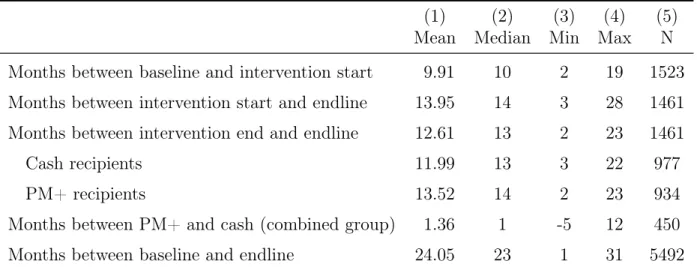
A baseline survey was conducted between October 2016 and March 2017, and an endline survey was conducted between August 2018 and May 2019. Online Appendix Table A.1 and Figure A.1 show an overview of the time elapsed, in months, between baseline and intervention start, intervention start/end and endline, and baseline and endline. The mean delay between the end of interventions and endline was 12.55 months, with a median of 13 months. The mean delay between the start of interventions and endline was 13.97 months (median: 14 months).
Both at baseline and endline, we conducted two surveys in each house-hold: a household survey, and an intimate partner violence (IPV) survey. The household survey contained modules on consumption, food security, assets, revenue, profits, labor, education, and psychological well-being. The IPV sur-vey contained questions on the prevalence of IPV, and norms around IPV. The household survey was given to the main respondent, as described above. At endline, the same respondent was re-surveyed. Note that this was the same person who received the intervention(s) in the treatment group. The IPV sur-vey was given to female respondents who were cohabiting with or married to a man; and to the female spouses or cohabiting partners of male respondents, on a different day than the household survey. It was always conducted by a
female FO, who took special care to ensure privacy due to the sensitive nature of the questions.
I.D.2 Variables
The full list of outcome variables is shown in Online Appendix Section I. Following our pre-analysis plan, we grouped our outcomes into four primary categories, and five secondary categories. The primary outcome categories were consumption, asset holdings, revenue, psychological well-being, and inti-mate partner violence. The secondary outcome categories were food security, profits, labor, and education. For each category, we computed a pre-specified index variable. In the case of monetary variables, this was usually the sum over a number of component variables, such as total household consumption or total asset holdings. For other variables it was a standardized weighted average following Anderson (2008). Monetary variables are winsorized at 1 percent and 99 percent.
Our primary outcomes are the following variables:
1. Monthly per-capita non-durable consumption (USD PPP): This variable measures total monthly expenditure on non-durables per capita, and the value of food consumption from own production, in USD PPP, dividing total household consumption by the number of household members (i.e. considering children as full adult equivalents). Sub-categories are food consumption (from own production and food bought); temptation goods; personal and household items; housing repair and improvement; and education expenditure, medical care, and social activities. The survey contained 134 food expenditure categories (recall horizon one week), 56 common non-food expenditure categories, such as airtime and firewood (recall horizon one month), and 9 low-frequency expenditure categories, such as weddings and school fees (recall horizon 12 months).
2. Total value of assets owned (USD PPP): This variable measures the total value in USD PPP of assets owned by the household. Sub-categories are productive assets, such as wheelbarrows and farming tools; vehicles,
such as bicycles and motorbikes; furniture; household durables, such as cell phones and kerosene stoves; livestock; and financial assets, i.e. savings and debt. The survey covered a total of 30 asset categories, and measures current value as estimated by the respondent (rather than purchase price).
3. Monthly household revenue (USD PPP): This variable measures total household revenue in USD PPP. Sub-categories are revenue from live-stock (e.g. milk and meat sales); income from crop sales; enterprise income (e.g. from kiosks); and wage income (e.g. from salaried jobs or casual labor).
4. Subjective well-being index (standard deviations): This variable is a standardized weighted average of several individual scales and questions: the General Health Questionnaire (GHQ-12; Goldberg and Blackwell 1970), a 12-item screener for general psychiatric conditions; the Per-ceived Stress Scale (PSS; 4 items, Cohen, Kamarck, and Mermelstein 1983); and the Happiness and Life Satisfaction questions from the World Values Survey (WVS). The standardized weighted average is computed following Anderson (2008), i.e. by overweighting variables which are less correlated with others and therefore presumably add more information. The WHODAS Disability Assessment Schedule 2.0, which measures dif-ficulties due to health conditions and is thus a function assessment, was analyzed as an additional, non-primary outcome that did not enter the index. The GHQ-12 has been used extensively to assess psychiatric mor-bidity in low- and middle-income countries, including Kenya, where it has been validated and used in previous randomized controlled trials, including that by Bryant et al. on PM+ (Abubakar and Fischer 2012; Getanda, Papadopoulos, and Evans 2015; Bryant et al. 2017). The PSS and WVS items have also been previously validated and used in Kenya (Haushofer and Shapiro 2016; Haushofer et al. 2020), and the same is true for the WHODAS (Bryant et al. 2017; Cresswell et al. 2020). The scales had good properties in our sample, with Cronbach’s alpha values
of 0.88 for GHQ-12, 0.60 for PSS, and 0.78 for WHODAS.
5. Intimate partner violence index (standard deviations): This variable is a standardized weighted average of two indices, one for physical and one for sexual violence. The physical violence index is a standardized weighted average of 9 variables measuring the frequency over the pre-ceding 6 months of various forms of violence perpetrated by the male intimate partner (usually the husband) against the female respondent, and against any children under 12 in the household. The sexual violence index is a standardized weighted average of variables measuring the fre-quency of rapes and other forced sexual acts committed by the intimate partner against the respondent over the preceding 6 months.
In explicit self-reports of IPV, we may worry about over- or under-reporting due to demand effects, e.g. arising from the perceived de-sirability of a particular response. We therefore supplement the explicit self-reports of IPV with two additional measures. First, an “envelope task” presented participants with 3 envelopes, of which two contained a yellow and one a red piece of paper. Participants were instructed to shuffle the envelopes and, without the surveyor watching, choose one and privately observe the color of the piece of paper it contained. They were then given two yes/no questions: one which they were supposed to answer if their envelope contained yellow paper, and another if their envelope contained red paper. Crucially, because the surveyor did not know the color of the paper, they did not know to which question the participant was responding. There were two rounds of this task. In the first round, the yellow question was: “In the past six months, have you ever visited a hospital or clinic?” The red question was: “In the past 6 months, has your husband ever beaten you, slapped you, or acted vio-lently against you?” In the second round, the red question was: “In the past 6 months, have you purchased any insurance or fertilizer?” The yel-low question was: “In the past 6 months, has your husband ever forced you to have sexual intercourse with him even when you did not want to?” In the analysis, we simply record the number of “yes” responses, knowing
that in expectation half of them are in response to the non-sensitive and the other half in response to the sensitive question. Decreases in violence would be reflected as decreases in the share of yes responses.
Second, in the “smiley task”, participants were presented with a sheet of paper with a happy face and a sad face on it, and asked to point to the sad face if the husband had beaten, slapped, or acted violently against them; and if the husband ever forced them to have sexual intercourse with him even when they did not want to in the past 6 months. We record whether participants point to the sad face, separately for each of these two questions.
The envelope task was presented first; the smiley task second; and the explicit questions last.
Our secondary outcomes were defined as follows:
1. Food security (standard deviations): This variable is a standardized weighted average of 6 variables measuring food security, such as the frequency over the preceding month of skipping meals, borrowing food from others, and eating protein.
2. Profits (USD PPP): This variable measures total household profits, i.e. revenue minus costs, from livestock, crops, and enterprises. Revenue is usually from sales, and costs include fodder, veterinary care, seeds, fertilizer, hired labor, etc.
3. Labor supply (hours): This variable measures the hours spent per week per capita on income-generating activities, including working in agricul-ture and tending animals, working in a non-farm or livestock business, and working for others. The per capita figure is obtained by dividing the total number of hours supplied by the household by the number of adults (older than 18) in the household.
4. Education (standard deviations): This variable is a standardized weighted average of the proportion of children enrolled in school; the average days of school missed per child in the preceding 30 days; the average spending
on school expenses per child in the preceding 12 months; and the average time spent studying or in school per child in the preceding 7 days. The variable is defined only for households with school-age children (between 5 and 19 years old).
The questionnaire contained a number of additional variables which were not pre-specified to be primary or secondary. Definitions for these variables are shown in the Online Appendix.
I.D.3 Data quality
Surveys were administered on tablet computers using the SurveyCTO sur-vey software. Data integrity was monitored through a series of checks: high-frequency checks, which checked incoming data for completeness on a weekly basis; back-checks, in which all survey respondents were re-surveyed within a week of the original survey to confirm a subset of presumably immutable responses, such as age or number of children; random spot checks in the field, i.e. visits and monitoring of surveys by supervisors; GPS checks, in which Google Earth was used to confirm the existence of a dwelling at the GPS lo-cations recorded in the survey; and M-Pesa confirmation, which consisted of confirming with Safaricom that the name of the respondent matched the name of the M-Pesa account. Further details are given in Online Appendix Section A.1.
II.
Econometric specifications
II.A
Direct and spillover effects
We use the following ANCOVA framework as our primary specification (McKen-zie 2012):
yvi = β0+ β1CTvi+ β2P M Pvi+ β3CT &P M Pvi+ β4DF Svi
+ β5SpillCTiv+ β6SpillP M P + γ0Xvi+ δyviB+ εvi
Here, yvi is an outcome for household i in village v; CTvi, P M Pvi, and
CT &P M Pvi are indicator variables for whether household i in village v
re-ceived a cash transfer, PM+, or both, respectively. SpillCTvi and SpillP M Pvi
are indicator variables for whether the household is a spillover household in
either cash transfer or PM+ villages. DF Svi is an indicator for whether the
household received an incentive to register for a mobile money account.13 X
vi
is a vector of stratification variables, including dummies for being female, having M-Pesa access, and being above the median at baseline on the psy-chological well-being index, the asset index, the IPV index, and village size.
yviB is the outcome variable at baseline; it was not collected for all outcomes,
in which case it is omitted. Where baseline data was collected but is miss-ing for some observations, we code the missmiss-ing value as zero and include a separate dummy variable indicating such replacements. Standard errors are clustered at the village level. The omitted category is households living in pure control villages who did not receive an incentive to register for a mo-bile money account. Note that the DF S treatment selected only households without M-Pesa access at baseline, and therefore including this indicator ef-fectively removes a number of respondents without M-Pesa at baseline from the sample. We therefore overweight respondents without M-Pesa accounts
accordingly. The coefficients β1, β2, and β3 identify the treatment effects of
the cash transfer, PM+, and combined intervention, respectively, relative to control. To test whether the interventions are complements, we test whether the sum of the treatment effects of the two individual interventions is smaller than that of the combined intervention, β1+ β2 < β3. The coefficients β5 and
β6 test whether cash transfers and PM+, respectively, have spillover effects.
To account for multiple hypothesis testing, we report False Discovery Rate (FDR) adjusted standard errors, correcting across our five primary outcome variables. We do not correct standard errors for multiple hypothesis testing for our secondary outcomes; for the individual variables that make up the primary and secondary outcomes; and for all other variables in the survey.
II.B
Baseline balance and attrition
To test for baseline balance, we estimate our standard treatment effect equa-tion 1 using baseline variables as outcomes (omitting baseline controls on the right-hand side). The baseline variables are constructed as follows: The base-line asset index is a standardized weighted average of responses to a shortened asset module administered at baseline. This module asked respondents if their household owns their home, land, a bed, mattresses, cell phones, cattle, oxen, bulls, goats, sheep, and savings. The baseline psychological well-being in-dex is a standardized weighted average of scores on the GHQ-12, stress, and WHODAS questionnaires. The baseline indices on IPV and justifiability of violence are constructed in the same way as their endline equivalents. Finally, we include variables for gender, age, and M-Pesa access at baseline.
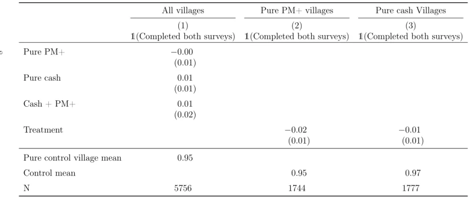
To test for differential attrition, we estimate the following model:
yvi= β0+ β1CTvi+ β2P M Pvi+ β3CT &P M Pvi+ γXvi+ δyviB+ εvi
Here, yvi is an indicator for participant i in village v completing both surveys.
The coefficients on CTvi, P M Pvi, and CT &P M Pvitherefore measure
differen-tial attrition across these treatment groups relative to pure control. Standard errors are clustered at the village level. To assess within-village differences in attrition, we include village-level fixed effects and restrict the sample to cash-only and PM+-only villages. Standard errors are not clustered.
II.C
Heterogeneous treatment effects
We test whether the effects of our treatments vary along the following pre-specified dimensions: baseline asset holdings; baseline intimate partner vio-lence index; gender of recipient; and baseline psychological distress. For re-cipient gender, the dimension of heterogeneity is a dummy variable for the main survey respondent being female. For the other dimensions, we create an indicator variable based on a median split. We then estimate estimate the
differential impact by including a dummy for the interactant, and interaction terms with all treatment arms, in the main specification (see Online Appendix Section D for details). Baseline psychological distress is measured as an in-dex composed of the WHO Disability Assessment Schedule (WHODAS) 2.0 and the GHQ-12, which are the measures used by the implementing NGO to diagnose psychological distress. In addition to the pre-specified median split cutoff on this measure, we also conduct an exploratory analysis in which we use the cutoff according to which the implementing NGO diagnoses individuals as having high distress. According to this criterion, individuals are classified as having high distress if their WHODAS score is greater than 2, which is the case for 40 percent of our participants at baseline; and having a GHQ-12 score above 16, which is the case for 30 percent of baseline respondents. Together, 33 percent of participants would have been classified as distressed at baseline according to the NGO’s criteria.
II.D
Demand effects
Our questionnaires rely on self-reports to measure treatment effects. This raises the concern that participants may alter their responses to “please” the experimenters, potentially leading to biased treatment effect estimates. To investigate whether such “experimenter demand effects” play a role in our study, we use the method proposed by De Quidt, Haushofer, and Roth (2018). This method bounds demand effects by deliberately inducing them through
“demand treatments”. In these treatments, participants are explicitly told
what the experimenters expect of them. We delivered such demand treatments to all respondents in the pure control group at endline, for three questions pertaining to physical violence, sexual violence, and depression. Each pure control respondent was allocated to either a “positive demand” or “negative
demand” treatment. Respondents in the “positive demand” treatment are
asked the following questions:
1. “We will now ask you questions about how your partner has acted towards you in the last 6 months. We hypothesize that people who participated
in this study and received the same treatment as you will give higher responses to these questions than others. How many times per month did your husband beat you, slap you or act violently against you?” 2. As above, but with the final question being: “How many times per month
did your husband physically force you to have sexual intercourse with him even when you did not want to?”
3. “I will read out a list of some of the ways you may feel or behave. Please indicate how often you have felt this way during the past week, using the following scale: Rarely or none of the time (<1 day); Some or little of the time (1-2 days); Occasionally or a moderate amount of time (3-4 days); All of the time (5-7 days). We hypothesize that people who participated in this study and received the same treatment as you will give higher responses to these questions than others. I felt depressed.”
Respondents in the “negative demand” treatment were asked the same ques-tions, except that the word “higher” was replaced with “lower”. The main idea behind the method by De Quidt, Haushofer, and Roth (2018) is experimenter demand is not a major issue if the “positive demand” and “negative demand” responses are similar. We test this by averaging the responses to the positive and negative demand questions and testing the difference in means using a t-test.
III.
Results
III.A
Baseline balance and attrition
We report estimates of baseline balance in Online Appendix Table A.2, and of attrition in Online Appendix Table A.3. We find no significant differences between these outcomes at baseline between any of our treatment groups and the control group. For the spillover groups, two coefficients are significant at the 10 percent level (psychological well-being was somewhat higher in the PM+ spillover group compared to control, and the justifiability of violence
somewhat lower in the cash spillover group compared to control). However, these differences are weak and the number of tests conducted relatively large, and we therefore do not regard this as evidence of imbalance. Our random-ization thus appears to have been successful in creating comparable treatment groups.
Online Appendix Table A.3 shows that we had 5 percent attrition between baseline and endline in pure control and PM+ villages, and 4 percent in cash and “Cash & PM” villages. The average completion rate of the endline
sur-vey for participants who completed baseline was 96 percent. These levels
of attrition are low and not statistically different from each other. Compar-ing treatment to spillover households within cash-only and PM+-only villages (columns (2) and (3)) also shows no differential attrition within treatment villages. Thus, we had low attrition overall, and it was not differential.
III.B
Treatment effects on primary and secondary
out-comes
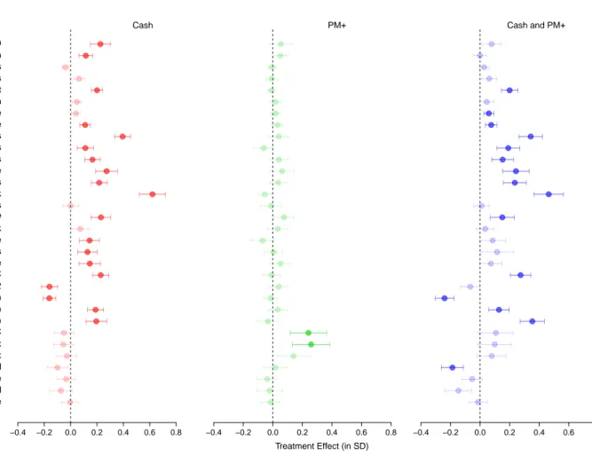
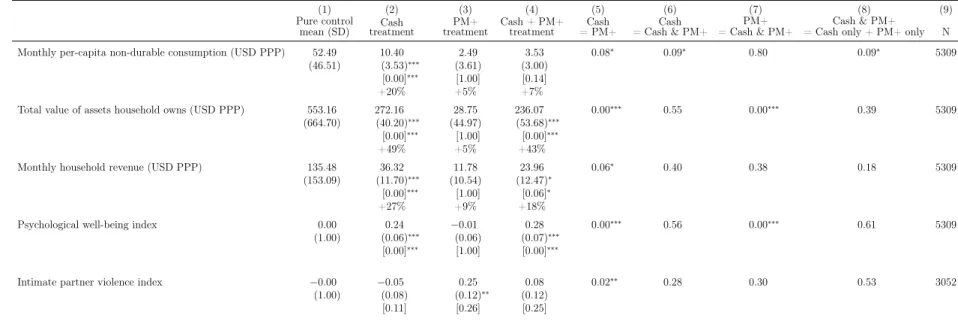
We next turn to treatment effects on our primary outcomes of interest, shown in Table 1 and Figure 3. Detailed tables are shown in Online Appendix Section B.1. Column (1) of Table 1 shows the pure control group mean and standard deviation; for standardized variables, the mean is zero and the standard devia-tion 1 by definidevia-tion. The cash transfer treatment has positive and statistically significant effects on 4 of our 5 primary outcomes, shown in column (2): con-sumption, asset holdings, revenue, and subjective well-being. The effect on consumption is a USD 10.51 PPP increase relative to a control group mean of 52.49, corresponding to a 20 percent increase. Similarly, the effect on assets is an increase of USD 262.06 PPP relative to a control group mean of 553.16, or a 47 percent increase. Revenue increases by USD 35.18 PPP per month, a 26 percent increase relative to the control group mean of USD 135.48 PPP. The subjective well-being index increases by 0.23 standard deviations (SD). All of these effects are significant at the 1 percent level using both naïve and FDR-adjusted p-values. We observe no significant effect on the intimate partner
violence index, which decreases by 0.05 SD.
The PM+ treatment, shown in column (3), has no significant effects on any of our primary outcomes except for intimate partner violence, where we observe an increase (i.e. a worsening of violence) of 0.24 SD. However, two caveats apply to this effect. First, it does not survive FDR correction. Second, as shown in Online Appendix Table B.5, when we use the envelope and smiley tasks to measure prevalence of IPV, we observe no significant increases in IPV. Thus, the impacts of the PM+ program on IPV are inconclusive. Nevertheless, future work should take seriously the possibility that PM+ might increase IPV, and attempt to provide more robust evidence and study possible mechanisms. The point estimates on consumption, assets, and revenue are positive, with a 5 percent increase in both consumption and asset holdings, and a 9 precent
increase in household revenue. However, these effects are not statistically
different from zero using both naïve and FDR-adjusted p-values. Using the 95 percent confidence intervals, we can rule out treatment effects larger than 18 percent on consumption, 21 percent on asset holdings, 24 percent on revenue, and 0.11 SD percent on psychological well-being. Column (5) reports the p-values testing the difference between the effects of the cash treatment and the PM+ treatment; all tests are statistically significant, suggesting that the cash treatment had significantly larger positive effects than the PM+ treatment.
Column (4) reports the treatment effect of the combined cash and PM+ treatment. These treatment effects are both numerically and statistically very similar to those of the cash-only treatment; for example, asset holdings in-creases by USD 227.61 PPP in the cash & PM+ group, a 41 percent increase relative to the control group mean, and similar to the USD 262.06 PPP treat-ment effect in the cash-only treattreat-ment. Similarly, revenue increases by USD 23.00 PPP, not too dissimilar to the USD 35.18 PPP increase in the cash-only treatment. The coefficient on the subjective well-being index is 0.27 SD, com-pared to 0.23 SD in the cash treatment. Only consumption shows a smaller effect, with a USD 3.62 PPP treatment effect in the combined treatment, com-pared to a USD 10.51 PPP treatment effect in the cash-only treatment. In the combined treatment, only the impacts on assets, revenue, and subjective
well-being are statistically significant (using both naïve and FDR-adjusted p-values), and the impact on revenue is only significant at the 10 percent level. Column (6) shows the difference between the cash treatment and the com-bined treatment, revealing that the impact on consumption is smaller in the combined than in the cash-only treatment (significant at the 10 percent level); the other effects are statistically similar.
Thus, the combined treatment has similar effects to the cash-only treat-ment, even though they are statistically somewhat less robust, and the con-sumption effect may in fact be smaller. All impacts in the combined treatment are numerically larger than those of the PM+ treatment, although as shown in column (7), only asset holdings and subjective well-being show statistically significant differences across the two treatment arms.
Finally, column (8) shows p-values comparing the sum of the treatment effects of the cash-only and PM+-only treatment arms to the effects of the combined treatment. With the exception of the consumption outcome, none of the p-values are statistically significant at conventional levels, which is not surprising given the small effects of the PM+ treatment and the similar effects of the cash-only and combined treatments. The summed effect on consumption is larger than the effect in the combined treatment arm, significant at the 10 percent level.
Table 2 reports effects on our secondary variables of interest. Mirroring the positive treatment effect of the cash transfer on consumption, we observe a 0.13 SD improvement in the food security index in this treatment arm, significant at the 5 percent level. We observe a 27 percent decrease in profits, but this effect is not statistically distinguishable from zero. Together with the positive effects on revenue, it suggests that cash transfer recipients grew their business, rather than increasing their profits. We see a small and insignificant reduction in labor supply, and a negligible effect on the education index. None of these effects are statistically significant, even with naïve p-values.
The PM+ treatment also has small and insignificant treatment effects on the secondary outcome variables, with numerically small reductions in food security, profits and working hours, and a small increase in the education
index. Again no result is statistically significant.
The combined cash and PM+ treatment also shows a significant increase in the food security index (0.12 SD). Apart from that, no coefficients are statistically significant, although there is a numerically relevant decrease in profits (−37 percent). Again this result corroborates the pattern that cash transfer recipients grew their businesses rather than increasing their profits. The other treatment effects are numerically small.
In line with the generally small impacts amongst these secondary outcome variables, the pairwise comparisons shown in columns (5)–(8) are not statisti-cally significant for the most part, with the sole exception of the food security index, which larger in the two treatment arms receiving cash than in the pure PM+ group.
III.C
Treatment effects on psychological well-being
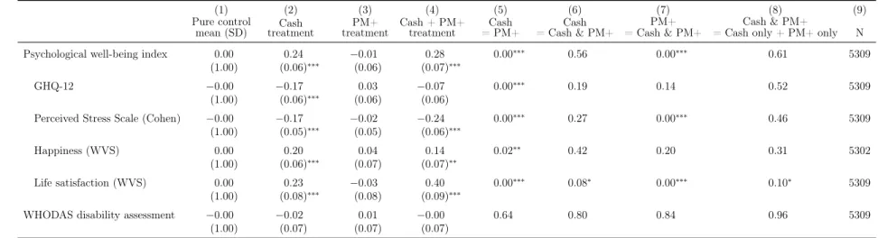
Table 3 reports the impacts on the individual psychological well-being vari-ables, all coded in standard deviations. The 0.23 SD effect of the cash transfer treatment on the subjective well-being index is driven by a 0.21 SD impact on life satisfaction; a 0.19 SD increase in happiness; and 0.16 SD decreases in the perceived stress and GHQ-12 scales. All effects are statistically significant. In contrast, the PM+-only treatment has no significant treatment effects on any of these variables, and all individual coefficients are smaller than 0.05 SD. The combined treatment has a similar effect on the psychological well-being index (0.27 SD) as the cash-only treatment (0.23 SD), and most individual impacts are also numerically similar. However, we observe a larger impact on life sat-isfaction in the combined treatment (0.39 SD) relative to the cash treatment (0.21 SD), with the difference significant at the 10 percent level. Thus, for this specific dimension, combining cash transfers with PM+ may have increasing returns, but the result needs replication. The function assessment, WHODAS, did not show significant treatment effects in any treatment arm.
Detailed treatment effects on other outcome groups are shown in Online Appendix Section B.1.
III.D
Interpreting null results: A Bayesian Approach
We briefly discuss what inferences can be drawn about the effectiveness of the PM+ program based on the largely null results we report above. For illustra-tive purposes, we focus on the effect of the PM+ program on the psychological well-being index. We first note that the standard error of the treatment effect is 0.06 SD, which means that we had 80 percent power to detect effect sizes
of 2.8 × 0.06 ≈ 0.17 SD at a significance level of 5 percent.14 This detectable
effect size is relatively small compared to treatment effects of psychotherapy reported throughout the literature. For instance, Cuijpers et al. (2010) report an average treatment effect of 0.67 SD in a meta-analysis of 117 randomized ex-periments comparing psychotherapy interventions to control conditions, which is still 0.42 SD after statistically adjusting for publication bias. For cognitive-behavioral therapy specifically, on which PM+ is based, Cuijpers et al. (2013) report a meta-analytic effect size estimate of 0.71 SD (no adjustment for pub-lication bias was undertaken). In the previous PM+ trial in Kenya, Bryant et al. (2017) report a 0.57 standard deviation (SD) improvement in the GHQ-12. Even allowing for the fact that PM+ is a low-dose, highly manualized version of CBT delivered by laypeople, the fact that we were powered to de-tect much smaller effects makes power an unlikely explanation of our findings. A natural question to ask is then what the probability is that the true effect of the PM+ program is smaller than 0.17 SD, our detectable effect size. This probability is given by the negative predictive value (NPV): the probability that there is no true effect of a given magnitude, given that no effect was detected with a given level of power and false positive probability. In addition to power and the false positive rate, the negative predictive value is influenced by priors, i.e. the probability we would have assigned to PM+ having an effect of at least 0.17 SD before the study. For power 1 − β (and thus false
14This insight uses the fact that to declare significance at 5 percent, the absolute value of
the test statistic must be larger than 1.96, and for this to be true with 80 percent probability, 80 percent of the sampling distribution from which test statistics are drawn must be to the right of 1.96. Because the 80 percent of the standard normal distribution is given by a z-score of 0.84, this is the case when the sampling distribution is centered 1.96 + 0.84 = 2.8 standard errors away from zero.
negative rate β), false positive rate α, and prior probability π, the NPV is given by Bayes’ theorem as the ratio of the expected rate of false negatives, (1−α)(1−π), to the expected rate of negative results overall, (1−α)(1−π)+βπ:
N P V = (1 − α)(1 − π)
(1 − α)(1 − π) + βπ
In our case, α = 0.05, and we calculated above that for an effect size of 0.17 SD, 1−β = 0.8. If we were completely agnostic as to whether PM+ is effective prior to the study (flat priors, π = 0.5), the post-study probability of PM+ having a true effect smaller than 0.17 is 0.83. With a prior of 90 percent in favor of PM+, the post-study probability against PM+ is 0.35. Thus, depending on the strength of our priors, the post-study probability of PM+ being ineffective is only moderately increased by our results. However, larger effects can be ruled out with greater confidence: even with a 90 percent prior in favor of its effectiveness, the post-study probability that PM+ produces effects smaller than 0.40 SD is 90 percent.
III.E
Cost effectiveness
The total amount paid to the NGO for the delivery of PM+ to the 1018 recipients (525 recipients in the PM+-only group, and 493 recipients in the combined group) was USD 1,210,107 (nominal), which includes both direct program cost and overhead. This corresponds to a program cost of USD 1,189 (nominal) per recipient. This cost is larger than the nominal amount of the cash transfers, USD 485, by a factor of 2.45. We conservatively assume that the costs of remitting the cash transfers, in M-Pesa and staff costs, amounted to 10 percent of the transfer value, for a cost of USD 534 per transfer. Using this cost, the PM+ program is more expensive by a factor of 2.27. The PM+ facilitators were paid KES 700 per session of PM+ administered, for a total of KES 3500 (USD 37 nominal, USD 75 PPP) across the five sessions of the program. At this marginal cost for PM+, the nominal amount of the cash transfer exceeds the marginal cost of PM+ by a factor of 14.43. The point
estimates of the cash transfer are larger than those of PM+ by factors of 4.17 (consumption), 10.04 (assets), and 3.04 (revenue). It is possible that the PM+ program would be substantially cheaper in the future, when infrastructure is already in place and CHWs are already trained; under such conditions, PM+ may be more cost-effective than cash transfers for these outcomes.
Online Appendix Figure C.1 illustrates the relative cost effectiveness of PM+ and cash transfers at different scenarios for the cost of PM+. For the purposes of this analysis, we take seriously the statistically non-significant, but positive impacts of PM+ on our monetary outcomes, i.e. consumption, assets, and revenue. (Note that for the other primary outcomes, the PM+ impacts have negative signs, while those of cash transfers are positive, making PM+ less cost-effective than cash transfers in all cost scenarios.) The horizontal axis represents different possible costs of delivering PM+ to a single recipient, ranging from marginal cost (USD 37 nominal) to total cost in this study (USD 1,189 nominal). On the vertical axis, we plot the ratio of the treatment effect of PM+ on monetary outcomes, per dollar spent on PM+, relative to the treatment effect of cash transfers on the same outcomes, per dollar spent on cash transfers (i.e. βˆ2/cP M P
ˆ
β1/534 , where cP M P is the varying cost of PM+, and
ˆ
β1 and ˆβ2 are the cash and PM+ treatment effect estimates from our main
estimating equation, respectively). The dotted vertical lines represent the
PM+ cost below which PM+ is more cost-effective in changing the outcome variable in question than cash transfers. We find PM+ may have the potential to be more cost-effective than cash transfers in improving revenue if the PM+ cost can be reduced to USD 175 per person; USD 128 for consumption; and USD 53 for assets.
III.F
Heterogeneous treatment effects
We report heterogeneous treatment effects of the cash transfer treatment, PM+ treatment, and the combined treatment on our primary outcomes in Online Appendix Tables D.1, D.2, and D.3, respectively. In Online Appendix Table D.1, we find that cash transfers generate a somewhat smaller effect on