Polymer Testing 99 (2021) 107220
Available online 1 May 2021
0142-9418/© 2021 The Author(s). Published by Elsevier Ltd. This is an open access article under the CC BY-NC-ND license (http://creativecommons.org/licenses/by-nc-nd/4.0/).
An empirical model for sorption by glassy polymers: An assessment of
thermodynamic parameters
Ivan Argatov
a,c,*, Vitaly Kocherbitov
b,c,** aCollege of Aerospace Engineering, Chongqing University, Chongqing, 400030, China bFaculty of Health and Society, Malm¨o University, SE-205 06, Malm¨o, SwedencBiofilms – Research Center for Biointerfaces, Malm¨o University, SE-205 06, Malm¨o, Sweden
A R T I C L E I N F O
Keywords: Sorption isotherm
Flory–Huggins interaction parameter Glass transition
A B S T R A C T
A new fitting model for sorption by glassy polymers is suggested based on the Flory–Huggins (FH) equation with a composite formula for the FH interaction parameter, χ, which is applicable if sorption experimental data shows a single-maximum variation of the FH parameter. Namely, a power-like and a linear approximation is assumed for χ(φ1), as a function of solvent volume fraction φ1, before and after the point of its maximum. After deter-mining the maximum point from a direct inspection of the sorption data, the three fitting parameters are evaluated by solving two independent least-square minimization problems. Several sorption studies of bio-polymers taken from the literature show that the endset of the glass transition region is correlated with the position of the maximum of the FH interaction parameter. Based on this hypothesis and the Vrentas–Vrentas model for sorption of glassy polymers, a theoretical framework for the glass transition analysis is developed. In particular, the solvent-induced glass transition temperature variation can be estimated from the sorption isotherm as a function of the solvent content corresponding to temperatures above the temperature of sorption.
1. Introduction
Sorption isotherm is an important characteristic for polymer mate-rials [1] as well as for food [2] and pharmaceutical [3] products, and a large number of analytical models (predictive and fitting) have been presented in the past to recast the experimental sorption data in an analytical form [4,5].
In the present work, we build upon the Flory–Huggins (FH) equation and suggest a piecewise-smooth approximation for the FH interaction parameter χ, which steams from the observation that a number of glassy
polymers exhibit a non-monotonic variation of χ as a function of the
solvent volume fraction φ1 with two different behaviors in the glassy and
rubbery states. The concept of concentration dependence of the Flor-y–Huggins parameter χ has been exploited in a number of previous
works (see, e.g. Refs. [6–8]). An innovation of the present study lies in the link of the smoothness discontinuity of χ to its local maximum.
The rest of the paper is organized as follows. In Section 2, we outline the developed modeling framework, which is partly based on the Vrentas–Vrentas theory [9]. The novelty of the suggested fitting model is in the use of a piecewise-smooth approximation for the FH interaction
parameter, for which we provide an interpretation in terms of thermo-dynamic parameters of the glassy state. Though, the composite fitting model shows a promising ability to approximate the sorption isotherm data, the originality of the present approach consists in the utilization of the fitting model for a further glass transition analysis aimed at extracting from the sorption isotherm valuable information, which re-quires performance of more experiments. In Section 3, a number of cases are treated by means of the suggested model in comparison with other models, including the three-parameter Guggenheim–Anderson–de Boer (GAB) model. Finally, in Section 4, we discuss the obtained results and formulate our conclusions.
2. Theory
2.1. The Flory–Huggins equation with a variable interaction parameter Let φ1 and φ2 denote the volume fraction of the solvent and polymer,
respectively. Then, the Flory–Huggins isotherm takes the form a1=φ1exp
( φ2+χφ22
)
, (1)
* Corresponding author. College of Aerospace Engineering, Chongqing University, Chongqing, 400030, China. ** Corresponding author. Faculty of Health and Society, Malm¨o University, SE-205 06, Malm¨o, Sweden.
E-mail addresses: ivan.argatov@gmail.com (I. Argatov), vitaly.kocherbitov@mau.se (V. Kocherbitov). Contents lists available at ScienceDirect
Polymer Testing
journal homepage: www.elsevier.com/locate/polytest
https://doi.org/10.1016/j.polymertesting.2021.107220
where a1=p1/p01 is the solvent activity, p1 is the pressure of the solvent, p0
1 is the saturation pressure of the solvent, and χ is the Flory–Huggins
(FH) interaction parameter.
While the FH equation (1) works well for polymers in the rubbery state at higher solvent volume fractions (and polymer solutions), it fails to accurately describe the sorption isotherm in the glassy state at low solvent concentrations.
In what follows, φ1g will denote the volume fraction of solvent at
which the experimental temperature, T, equals the glass transition temperature, which is denoted by Tgm.
According to Vrentas and Vrentas [9], Eq. (1) can be generalized as follows: a1=φ1exp ( φ2+χ0φ22 ) exp(F). (2)
Here, χ0 is a constant, the exponent F is a function of the solvent volume fraction φ1, such that F(φ1g) =0 and F(φ1) <0 for φ1∈ (0,φ1g).
We note that another generalization of the FH equation is due to Leibler and Sekimoto [10] who presented their isotherm in the glassy regime in the form of Eq. (2) but with different expression for the exponent F, which however satisfies the same non-positivity condition.
Observe that by the introduction of the variable interaction param-eter χ=χ0+ F φ2 2 , (3)
the form of Eq. (2) will exactly coincide with Eq. (1). It is important to observe that since F(φ1) <0 for φ1<φ1g and F(φ1) =0 for φ1≥φ1g, the
function χ(φ1)defined by (3) has at φ1=φ1g the value χ(φ1g) =χ0 that coincides with the maximum of χ(φ1). The use of a concentration dependent FH interaction parameter is a requirement for non- equilibrium systems in order to describe the experimental behavior in conditions not suitable for the application of the FH model.
This obvious observation suggests to study the variation of the FH interaction parameter. The following simple formula allows to evaluate the variable value of χ directly from the experimental data [1]:
χ=ln(a1/φ1) − φ2
φ2 2
. (4)
It is pertinent to mention here that φ2 =1 − φ1. We should also note
here that in principle Eq. (4) follows from Eq. (1) directly, and is not related to Eq. (2).
2.2. Piecewise-smooth approximation for the Flory–Huggins parameter The problem of extracting glass transition temperatures from equi-librium solvent sorption data was discussed by Bell [11], whose exper-imental results on moisture sorption by polyvinylpyrrolidone suggest that glass transition data cannot be distinguished from moisture sorption isotherms without extensive knowledge about the system. However, it is important to note that per se only the visual estimation of the upper inflection range was used [11] to associate the moisture-induced glass transition with the moisture isotherm.
In the present study, we consider the variable FH parameter (4) as an indicator for the presence of the solvent-induced glass transition.
Let χ∗denote the maximum of the FH interaction parameter, that is
χ∗=maxχ(φ1), χ∗=χ(φ1∗). (5)
Then, based on the analysis of the experimental data (see Section 3), the following approximation is suggested:
χ(φ1) = { χ∗− α(φ1∗− φ1) ν , φ1≤φ1∗, χ∗− β(φ1− φ1∗), φ1≥φ1∗. (6)
Here, α, β, and ν are fitting parameters.
The results of the application of the piecewise-smooth approximation
are presented in Section 3. 2.3. Postpredictive analysis
After making use of Eqs. (1) and (6) for fitting a given set of exper-imental sorption data, we can apply the Vrentas–Vrentas model for extracting valuable information from the sorption isotherm. First, by identifying the glass transition with the state of maximum of the FH parameter, that is by assuming that
φ1g=χ∗, χg=χ∗, (7)
formulas (A.14) and (A.15) will provide an estimate for the specific heat capacity change ΔCp= qRT M1Tg2 ( 1 − T Tg2− T Tg2ln Tg2 T )−1∫φ1g 0 ( χg− χ ) dφ1, (8)
where χ as a function of φ1 is given by the left part (φ1≤φ1∗) of formula (6).
It is worth noting here that formula (8) can be applied irrespectively of the fitting model (1), (6) by numerically evaluating the integral in (8) for the FH parameter χ(φ1)obtained directly from the experimental data suing Eq. (4).
2.4. Further, let us introduce the auxiliary notation f (φ1) = q ΔCp RT M1 ( χg− χ(φ1) ) . (9)
Then, Eqs. (A.6) and (A.10), in view of (7), yield ( T Tgm − 1 ) dTgm dφ1 =f (φ1), (10)
where 0 ≤ φ1≤φ1g, and f(φ1)is given by (9).
Equation (10) can be regarded as a differential equation for deter-mining Tgm as a function of φ1, since the right-hand side of Eq. (10), in
view of (8) and (9), van be evaluated from the experimental sorption data either directly or after fitting with formula (6).
Thus, integrating Eq. (10) with the initial condition Tgm|φ1=0 =Tg2,
we obtain Tg2− Tgm− Tln Tg2 Tgm = ∫φ1 0 f (φ) dφ. (11)
Equation (11) determines the function Tgm(φ1)in the implicit form, and the evaluation of Tgm(φ1)for a given φ1∈ (0, φ1g)requires solving
the transcendental equation (11), which can be done by numerical methods.
Observe that, in view of (9), the right-hand side of Eq. (11) depends on ΔCp, which is not always readily available. That is why, another form
of Eq. (11) will be also useful. For this, we put X(φ1) = ∫φ1 0 ( χg− χ(φ) ) dφ. (12)
Then, taking into account Eqs. (8), (9) and (12), we can rewrite Eq. (11) as follows: 1 − Tgm Tg2 − T Tg2 lnTg2 Tgm =X(φ1) X(φ1g ) ( 1 − T Tg2 − T Tg2 lnTg2 T ) . (13)
We note that according to (6) and (7), the integral (12) can be simply evaluated as
X(φ1) = α 1 +ν [ φ1+ν 1g − ( φ1g− φ1 )1+ν] . (14)
2.5. From Eq. (14), it follows that X(φ1) X(φ1g ) = 1 − ( 1 − φ1 φ1g )1+ν , (15)
and therefore, Eq. (13) can be simplified further.
Thus, in view of (13) and (15), the fitting parameter ν characterizes
the glass transition temperature variation as a function of the absorbed solvent fraction.
3. Fitting of experimental data and comparison with other models
3.1. Fitting performance of the proposed model
To test the aptness of the suggested fitting model, we considered a number of examples of hydration of different polymers taken from the literature. The model’s fitting performance is compared to those of the Guggenheim–Anderson–de Boer (GAB) model and the five parameter Park’s model [12]. We recall that the GAB model can be written for the equilibrium moisture content, r1, as
r1=
k1k2k3a1
(1 − k3a1)[1 + (k2− 1)k3a1]
, (16)
where r1 is the absorbed mass ratio defined as the ratio m1/m2 of the
mass of absorbed water, m1, to the mass of dry polymer, m2. The fitting
parameters are interpreted as follows [13]: k1 is the mass ratio
corre-sponding to a monolayer of absorbed water, k2 is the Guggenheim
constant, and the parameter k3 accounts for the modified properties of
sorbate in the multilayer region.
The five-parameter model of Park [12] takes the form r1=
k1k2a1
1 + k2a1
+k3a1+k4ak15, (17)
where the fitting parameters are interpreted as follows [13]: k1 is the
Langmuir capacity constant, k2 is the Langmuir affinity constant, k3 is
the Henry’s type solubility coefficient, k4 is the equilibrium constant for
the clustering reaction, and k5 is the mean number of water molecules
per cluster.
To quantify the quality of fitting performance, the following three error measures are used:
MAPE =100 N ∑N i=1 ⃒ ⃒Afit i − A exp i ⃒ ⃒ Aexpi , χ2= ∑N i=1 ( Afit i − A exp i )2 Afit i , (18) HYBRIDp= 100 N − p ∑N i=1 ( Afit i − A exp i )2 Aexp i , (19)
where N is the number of data points, Aexp
i and Afiti are the
experimen-tally measured and calculated (fitted) values of the physical quantity in question, and p is the number of the fitting parameters.
The mean absolute percentage error (MAPE) has a simple and intu-itive interpretation as the mean value for the relative errors. The chi- square test was recommended [14] for comparing the isotherms on the same abscissa and ordinate. The hybrid fractional error function (HYBRID) [15] accounts for different number of fitting parameters in the models under consideration.
3.2. Fitting algorithm
The algorithm of fitting Eqs. (1), (6) to a given soprtion data can be
formulated as follows. Given a data set a1i and w1i (or r1i), i = 1, 2,…,N,
and the dry polymer density d2, we evaluate the corresponding array of
the solvent volume fraction φ1i, using one of the following formulas:
φ1i= w1i q + (1 − q)w1i , φ1i= r1i q + r1i . (20)
3.3. Here, q = d1/d2, and volume additivity is assumed Second, using formula (4), we evaluate the FH parameter as χ1i=
ln(a1i/φ1i) − 1 + φ1i
(1 − φ1i)
2 , (21)
and determine the maximum χ∗=maxi {χ1i} and the corresponding
number n∗, such that χ∗=χi and φ1∗=φ1i for i = n∗.
Then, we define the left and right approximations for the FH inter-action parameter
χL(φ1,α,ν) =χ∗− α(φ1∗− φ1)
ν
, φ1≤φ1∗, (22)
χR(φ1,β) =χ∗− β(φ1− φ1∗), φ1≥φ1∗. (23)
The substitution of formulas (22) and (23) into Eq. (1) yields the analytical approximations for the water activity
a1L(φ1,α,ν) =φ1exp { 1 − φ1+χL(φ1,α,ν)(1 − φ1) 2}, (24) a1R(φ1,β) = φ1exp { 1 − φ1+χR(φ1,α,ν)(1 − φ1)2 } , (25)
which are valid for φ1≤φ1∗and φ1≥φ1∗, respectively.
The corresponding functionals of summed square errors are defined in a usual way as EL(α,ν) = ∑n∗ i=1 (a1L(φ1i,α,ν) − a1i)2, (26) ER(β) = ∑N i=n∗ (a1R(φ1i,α,ν) − a1i)2. (27)
Next, the optimal values, α∗, ν∗, and β∗, of the fitting parameters are
determined, respectively, by solving the two minimization problems min
α,νEL(α,ν) = EL(α∗,ν∗), minβ ER(β) = ER(β∗).
It is worth to mention here that, though the fitting model (24), (25) contains five parameters, three of which are adjustable constants, the fitting procedure per se reduces to solving one two-parameter and one one-parameter least-square minimization problems, which can be solved independently. This fact explains that the associated fitting algorithm, which is outlined above, is robust and stable.
3.4. Comparison with the Vrentas–Vrentas model
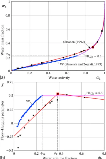
We consider the experimental and theoretical results presented by Hancock and Zografi [16] for water sorption by poly(vinylpyrrolidone) (PVP) at T = 25∘C. Besides the experimental data and our fit to them
using Eqs. (1) and (6), Fig. 1a also shows the predictions made according to the Vrentas–Vrentas (VV) model (2), (A.1). It is important to under-line here that the application of the VV model requires the knowledge of the function Tgm(w1)for w1≤w1g, where w1g is the water mass fraction which is sufficient to lower the glass transition temperature of the pol-ymer/water system to that of its environment, i.e., Tgm(w1g) =T. The corresponding volume fraction is denoted by φ1g.
When the sorption data is recalculated in terms of the FH parameter using Eqs. (3) and (4), the discrepancy between the models becomes more evident (see Fig. 1b). It is interesting that the shape of the VV- corrected FH parameter (which is denoted by the dotted blue line) is
similar to that of the experimentally observed variation (which is denoted by black squares). As it was noted [16], the function Tgm(w1) and its derivative Tgm/dw1 are most critical in determining the shape of
the sorption isotherm below w1g.
Fig. 1b clearly demonstrates the main difference between the VV model and our approach. First, while the VV model in the rubbery state assumes that χ0 =const, we employ a linear approximation for the FH parameter. Second, while the transition between the glassy and rubbery states in the VV model is supposed to be known from sources other than the sorption isotherm, in our approach the point of transition from a glassy state to a rubbery state (that is φ1g in terms of volume fraction) is
identified based on the position of maximum FH parameter (that is φ1∗
in terms of volume fraction). We would like to emphasize that this cri-terion does not contradict to the VV model, as it can be seen from Fig. 1b, the FH parameter reaches its maximum when the water volume fraction φ1 approaches φ1g from the left. Third, whereas the model of Vrentas and Vrentas [9] is a predictive model, and therefore, the observed poor fit in Fig. 1a can be attributed in part to uncertainty in the required data (namely, ΔCp and Tgm(w1)), our fitting model has a strong potential for
the glass transition analysis, as it will be demonstrated below. 3.5. Sorption-desorption hysteresis of mucin
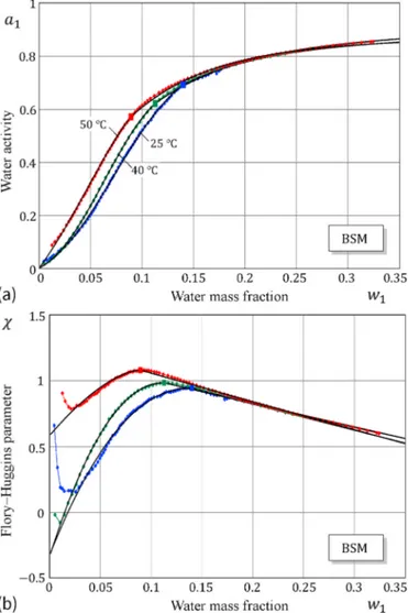
We consider the water sorption-desorption isotherms of bovine submaxillary gland mucin (BSM) films with nanoscale thicknesses studied by Bj¨orklund and Kocherbitov [17], using humidity scanning quartz crystal microbalance with dissipation monitoring (QCM-D). The density of dry BSM mucin film is taken to be d2 =1.08 g/cm3. Fig. 2a shows that the onset of the sorption-desorption hysteresis in excellent agreement with the points of maxima of the FH interaction parameter. It is interesting to observe (see Fig. 2b) that the shapes of the FH parameter in the glassy state is different for sorption (α=73.304, β = 0.572, ν=2.489) and desorption (α=19.880, β = 0.629, ν=1.347), which manifests itself in different values for the exponent ν.
Let us briefly consider the application of the model of Vrentas and Vrentas [18] for describing hysteresis effects in sorption by glassy polymers. According to the VV model, Eqs. (2), (A.1) apply for modeling the functional relation between the water volume fraction φ1 and the
water activity in sorption a1,s, whereas in desorption Eq. (2) should be
modified as follows: a1,d=φ1exp ( φ2+χ0φ22 ) exp(kF). (28)
Here, k is an empirical coefficient.
According to Eqs. (3) and (28), we introduce the variable FH pa-rameters in sorption and desorption as
χs=χ0+ F φ2 2 , χd=χ0+ kF φ2 2 . (29)
Since the VV exponent F is a function of water content, which is specified by φ1, and vanishes at the glass transition, φ1 =φ1g, the
pa-rameters χ0 and φ1g are determined from the point of maximum of the
FH parameter χs(φ1), i.e., χ0=maxχs(φ1) and φ1g is such that χ0 = χs(φ1g).
After that the factor F can be evaluated from the sorption data as follows: F = ln ( a1,s φ1 ) − 1 + φ1− χ0(1 − φ1)2. (30)
Then, making use of Eqs. (2) and (28), we arrive at the following formula [17]: k = 1 +1 Fln ( a1,d a1,s ) . (31)
The behavior of the VV parameters F and k is shown in Fig. 2c, from where it is seen that the parameter k is not constant in the whole range of water contents of the glassy state. It is to note here that based on the analysis of the variations of the model fitting parameters, the proposed fitting model provides an approach to study typical features of glassy polymers sorption such as ageing, conditioning, and annealing. 3.6. Sorption by starch
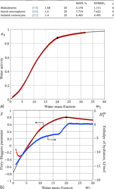
We consider the hydration of untreated spray-dried acid hydrolyzed starch (maltodextrin) studied by Carlstedt et al. [19], using sorption calorimetry. Observe (see Fig. 3a) that the sorption isotherm exhibits the step related to a crystallization phase transition, which is not taken into account in fitting the main part of the sorption isotherm.
By using Eqs. (1) and (6), we readily obtain α=114.86, β = 0.403, and ν=2.754. The corresponding fitting errors are presented in Table 1. Now, we consider the hydration of cross-linked starch microspheres studied by Wojtasz et al. [20], using sorption calorimetry at room temperature (see Fig. 4a). By using Eqs. (1) and (6), we obtain α= 17.530, β = 0.670, and ν=1.92. The corresponding fitting errors are presented in Table 1.
Fig. 1. Sorption of water by poly(vinylpyrrolidone) (PVP) at 25 ∘C according to
the sorption data presented by Hancock and Zografi [16]: a) Sorption isotherm data (black squares) fitted by the Vrentas–Vrentas (VV) model (2), (A.1) (dotted blue line continued by the FH isotherm) and the model (1), (6) (red solid line with the large red square denoting the location of the maximum of the FH parameter χ); b) The variation of the FH interaction parameter. (For interpre-tation of the references to colors in the figure legends, the reader is referred to the web version of the article.). (For interpretation of the references to color in this figure legend, the reader is referred to the Web version of this article.)
By comparing the variation of the FH interaction parameter with the evolution of the enthalpy of hydration (See Figs. 3b and 4b), which in both cases exhibits a pronounced glass transition, we come to the following conclusion. The point φ1∗of maximum FH parameter χ(φ1) can be identified with the point φ1g of solvent-induced glass transition at
experiment temperature T, though the glass transition predicted from maxχ(φ1)is more close to the endset of the glass transition region.
3.7. Sorption by corneocytes
Another case of water sorption published in the literature, for which we have access to row data, is the hydration of corneocytes isolated from the pig skin studied by Silva et al. [21] at room temperature, using sorption calorimetry.
By using Eqs. (1) and (6), we obtain α=22.864, β = 0.641, and ν= 1.972 for the sorption isotherm shown in Fig. 5a. The corresponding fitting errors are presented in Table 1. By comparing the variation of the FH interaction parameter with the evolution of the enthalpy of hydra-tion (See Fig. 5b), which exhibits a noticeable glass transition, we may Fig. 2. Sorption of water by mucin at room temperature according to the
hu-midity scanning QCM-D data of Bj¨orklund and Kocherbitov [17]: a) Sorption-desorption isotherms fitted by the model (1), (6) (large black dot and blue square denote the location of the maximum of the FH parameter χ for sorption and desorption, respectively); b) The variations of the FH interaction parameter; c) The variations of the Vrentas–Vrentas (VV) exponent (left ordi-nate axis) and the VV factor (right ordiordi-nate axis) as functions of the water mass fraction. (For interpretation of the references to color in this figure legend, the reader is referred to the Web version of this article.)
Fig. 3. Sorption of water by untreated spray-dried acid hydrolyzed starch at 25
∘C according to the sorption microcalorimetry data of Carlstedt et al. [19]: a)
Sorption isotherm data (red triangles) fitted by the model (1), (6) (large black dot denotes the location of the maximum of the FH parameter χ); b) The FH interaction parameter (left ordinate axis) compared to the partial molar enthalpy of mixing (right ordinate axis). The shaded region represents the range that was not accounted for in fitting the sorption isotherm. (For interpretation of the references to color in this figure legend, the reader is referred to the Web version of this article.)
formulate the following conclusion. The point φ1∗ of maximum FH
parameter χ(φ1)can be identified with the point φ1g of solvent-induced glass transition at experiment temperature T, though again the glass transition predicted from maxχ(φ1)is found to be close to the endset of the glass transition region.
The observed above correlation of the maximum of χ(φ1)with the glass transition has been verified against the hydration studies of the stratum corneum (SC) and corneocytes isolated from the pig ears con-ducted by Mojumdar et al. [22] at 32 ∘C, using sorption microbalance
measurements (see Fig. 6a). It is interesting the variations of the FH interaction parameter for intact SC (α=140.24, β = 0.958, ν= 2.15) and isolated corneocytes (α=18.691, β = 0.900, ν= 1.682) show a
somewhat similar trend, though the locations of maxima are markedly different (see Fig. 6b).
It is interesting that the maximum of χ(φ1)in the case of corneocytes is strongly associated with the abrupt start of increase in the keratin d- spacing, which was measured by wide-angle X-ray diffraction (WAXD) (see Fig. 6c). At the same time, the keratin interchain spacing measured in intact SC obviously does not correlate with the corresponding maxχ(φ1). On the other hand, the water sorption calorimetry studies of Silva et al. [21] showed that the partial molar enthalpy of mixing curve for the intact SC does not exhibit any pronounced steps that would indicate phase transitions.
Table 1
Comparison of the fitting model (1), (6) with the GAB (Guggenheim–Anderson–de Boer) model (16) and the Park model for several binary polymer/water systems.
Polymer Ref. d2, g/cm3 T,∘C GAB model Park’s model New model
MAPE,% HYBRID3 χ2 MAPE,% HYBRID5 χ2 MAPE,% HYBRID5 χ2
Maltodextrin [19] 1.68 25 3.178 1.111 0.855 1.098 0.142 0.100 1.265 0.274 0.184
Starch microspheres [20] 1.6 25 7.719 7.621 9.063 2.458 0.792 0.947 1.924 0.582 0.543
Isolated corneocytes [21] 1.4 25 6.465 4.491 4.688 2.879 0.709 0.799 0.729 0.177 0.180
Fig. 4. Sorption of water by cross-linked starch microspheres at 25 ∘C
ac-cording to the sorption microcalorimetry data of Wojtasz et al. [20]: a) Sorption isotherm data (red triangles) fitted by the model (1), (6) (large black dot de-notes the location of the maximum of the FH parameter χ); b) The FH inter-action parameter (left ordinate axis) compared to the partial molar enthalpy of mixing (right ordinate axis). (For interpretation of the references to color in this figure legend, the reader is referred to the Web version of this article.)
Fig. 5. Sorption of water by isolated corneocytes at 25 ∘C according to the
sorption microcalorimetry data of Silva et al. [21]: a) Sorption isotherm data (red triangles) fitted by the model (1), (6) (large black dot denotes the location of the maximum of the FH parameter χ); b) The FH interaction parameter (left ordinate axis) compared to the partial molar enthalpy of mixing (right ordinate axis). (For interpretation of the references to color in this figure legend, the reader is referred to the Web version of this article.)
3.8. Prediction of the glass transition temperature variation for maltodextrin
We consider the water sorption data for maltodextrin DE 10 at 25 ∘C
obtained by Nurhadi et al. [23], using salt sorption technique. By putting d2 =1.37g/cm3, we find that the application of Eqs. (1) and (6) to the data yields the maximum point φ1∗ =0.175, χ∗=0.945 and the fitting
parameters α=49.554, β = 0.304, ν=1.757 with the following fitting errors: MAPE = 1.409, HYBRID3 = 3.687 × 10⁻³, and HYBRID
5 =
6.145 × 10⁻³. We note that the large difference between the latter two
error measures is explained by the low number of data points (N = 8), so that the factor 100/(N − p) in formula (19) is equal to 100/(8 − 3) = 20 and 100/(8 − 5) = 33.3 for p = 3 and p = 5, respectively.
In principle, the proposed fitting model (1), (6) can be applied in a relaxed version by regarding φ1∗ and χ∗as free parameters. By
intro-ducing the positive part function (x)+ =0.5(x + |x|), we can rewrite
formula (6) as χ(φ1) =χ∗− α(φ1∗− φ1)
ν
+− β(φ1− φ1∗)+, (32)
where the volume fraction φ1 takes all admissible values.
Now, we apply formula (32) with five fitting parameters. In doing so, we obtain α=25.493, β = 0.318, ν=1.408, φ1∗ =0.164, and χ∗=
0.952 with the following fitting errors: MAPE = 1.013 and HYBRID5 = 5.166 × 10⁻³. The result of the relaxed fitting is shown in Fig. 7a, where
the GAB curve is drawn according to the parameters given in Ref. [23]. This example shows (see Fig. 7b) that, generally speaking, the point of maximum of the FH parameter may not coincide with one of the data points.
Further, using the value Tg2=147∘C taken from Ref. [23] and
applying Eqs. 13 and 15, we can predict the glass transition temperature variation in the range of temperature above T = 25∘C, that is in the
range of mass ratio r1∈ (0, r1g), where r1g=0.143 that corresponds to φ1g =0.164. The predicted glass transition temperature Tgm is found to
be very close to the experimental data, which are also well fitted by the Gordon–Taylor equation according to the parameters given in Ref. [23]. 3.9. Prediction of the glass transition temperature of dry mucin
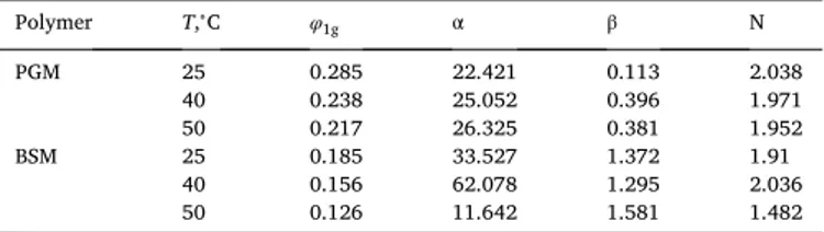
Finally, we consider the hydration of pig gastric mucin (PGM) and bovine submaxillary gland mucin (BSM) studied by Znamenskaya et al. [24], using sorption and differential scanning calorimetry at different temperatures. The application of Eqs. (1) and (6) to the sorption data yields the results presented in Table 2 and shown in Figs. 8 and 9.
In Fig. 10a, we compare the variation of the FH interaction param-eter with the evolution of the enthalpy of hydration (measured at 40 ∘C)
to illustrate the relation between the glass transition regions and the location of the maxima of the FH parameter.
Finally, using the evaluated data and Eq. (13), we estimate the Tg2 for
dry mucin by the one-parameter least-square regression analysis (under the assumption that Tg2 is greater than 25 ∘C). The density of dry mucin
films is taken to be d2 =1.4 g/cm3. The corresponding numerical re-sults are presented in Fig. 10b. The obtained values Tg2=571.9 K (PGM) and Tg2=456 K (BSM) are very close to the lower bounds in the corresponding estimates Tg2=610 ± 70 K (PGM) and Tg2=655 ± 181 K (BSM) obtained by Bj¨orklund and Kocherbitov [17]. At the same time, it should be noted that the opposite relation TPGM
g2 >Tg2 BSMhas been
found between the newly predicted glass transition temperatures of the two different types of mucin. Moreover, the difference between them has increased compared to the average results produced in Ref. [17]. Thus, more accurate estimation of these values requires a further study. 4. Discussion and conclusions
Overall, the proposed fitting model is capable of obtaining a good Fig. 6. Sorption of water by corneocytes and stratum corneum at 32 ∘C
ac-cording to the dynamic vapor sorption data of Mojumdar et al. [22]: a) Sorption fitted by the model (1), (6) (large squares denote the location of the maximum of the FH parameter χ); b) The variations of the FH interaction parameter; c) The FH interaction parameter (left ordinate axis) compared to the keratin d–spacing (right ordinate axis), which are measured for corneocytes and stra-tum corneum. Same legend as in figure (a) applies also in figures (b) and (c).
quality of fitting sorption isotherms for glassy polymers, as it can be seen from Table 1.
Observe that the point of maximum FH parameter is found to be located close to the endset of the glass transition interval. This conclu-sion is supported by an almost linear variation of χ(φ1), when φ1 is greater than φ1g. However, a closer inspection of the water sorption
scanning isotherms represented, e.g., in Figs. 3a, 4a and 8a, and 9a, implies that the linear approximation χR(φ1) =χ∗− β(φ1− φ1∗)can be
improved by allowing the sorption curve to exponentially approach a straight asymptote in the rubbery state. The corresponding refined approximation introduces two additional fitting parameters. However, by improving the fit to the sorption data in the rubbery region, one does Fig. 7. Sorption of water by maltodextrin DE 10 at 25 ∘C according to the salt
sorption data of Nurhadi et al. [23]: a) Sorption fitted by the model (1), (6) with free model parameters χ∗and φ1∗ (large red dot denotes the location of the
maximum of the fitted FH parameter χ). Solid dark green line represents the Guggenheim–Anderson–de Boer (GAB) model; b) The variation of the FH interaction parameter; c) The variation of the lass transition temperature fitted by the Gordon–Taylor (GT) equation. The solid red line is drawn by formula (13). (For interpretation of the references to color in this figure legend, the reader is referred to the Web version of this article.)
Table 2
Fitting parameters for the water sorption isotherms of PGM and BSM shown in
Figs. 8a and 9a, which are based on the data from Ref. [24].
Polymer T,∘C φ 1g α β N PGM 25 0.285 22.421 0.113 2.038 40 0.238 25.052 0.396 1.971 50 0.217 26.325 0.381 1.952 BSM 25 0.185 33.527 1.372 1.91 40 0.156 62.078 1.295 2.036 50 0.126 11.642 1.581 1.482
Fig. 8. Hydration of pig gastric mucin (PGM) according to the sorption microcalorimetry data of Znamenskaya et al. [24]: a) Sorption isotherms data fitted by the model (1), (6) (large squares denote the locations of the maximum of the FH parameter χ); b) The corresponding FH interaction parameters.
not affect the model parameters α and ν that primarily characterize the
glassy state.
Another modification of the main fitting algorithm would be to let the point (φ∗,χ∗)be free, and this is, as a rule, recommended in the case
of salt sorption with only a few data points (see Section 3.7). In the case of scanning sorption, this approach allows to adjust the position of the start of the linear approximation in the rubbery state. It worths noting that the piecewise-smooth expression (32) is differentiable and, in particular, we have ∂χ ∂φ1∗ = − να(φ1∗− φ1) ν−1 + +βH (φ1− φ1∗),
where H (x) is the Heaviside step function, defined as unity for positive and zero for negative values of the argument x.
The results presented here are compared with the sorption calori-metric data (which provide direct information about the isothermal glass transition). These sorption calorimetric data were earlier compared with DSC data and a good agreement was demonstrated (see for example the phase diagram in Ref. [19]). Moreover, due to un-certainties in associated with DSC sample preparations and experiments, the presented method can provide more accurate data on the glass transition concentration at a given temperature.
To conclude, based on the FH equation, the new fitting model for
sorption isotherm of glassy polymers is suggested by approximating the FH interaction parameter with a piecewise-smooth function. By deter-mining the point of maximum of the FH parameter via a direct inspec-tion of the sorpinspec-tion data, the three fitting parameters of the model α, β,
and ν are determined using two independent least-square minimization
problems (one two-parameter problem for α, β and one one-parameter
model for ν). A number of examples of sorption and calorimetry
studies, it is shown that the maximum point of the FH parameter is considerably correlated with the endset of the glass transition region. Based on the Vrentas–Vrentas theory and the fitted sorption isotherm, analytical approximations are derived for the change in specific heat of the solute across glass transition and the variation of the solvent-induced glass transition temperature.
Declaration of competing interest
The authors declare that they have no known competing financial interests or personal relationships that could have appeared to influence the work reported in this paper.
Fig. 9. Hydration of bovine submaxillary gland mucin (BSM) according to the sorption microcalorimetry data of Znamenskaya et al. [24]: a) Sorption iso-therms data fitted by the model (1), (6) (large squares denote the locations of the maximum of the FH parameter χ); b) The corresponding FH interac-tion parameters.
Fig. 10. Hydration of PGM and BSM at 40 ∘C according to the sorption
microcalorimetry data of Znamenskaya et al. [24]: a) The FH interaction parameter (left ordinate axis) compared to the partial molar enthalpy of mixing (right ordinate axis). The arrows denote the onsets and endsets of the glass transition regions; b) Prediction of the glass transition temperature based on the optimal fit by equation (13) (solid and symbolized lines correspond to Eqs. (15) and (12), respectively).
Acknowledgment
This research was carried out in the Biobarriers profile and was
funded by the Knowledge foundation (KK-stiftelsen). The authors thank Professor Johan Engblom for fruitful discussions.
Appendix. Interpretation via the Vrentas–Vrentas theory
According to Vrentas and Vrentas [9], the additive term F that enters Eq. (2) has the form F = − w2 2ΔCp M1 RT dTgm dw1 ( T Tgm − 1 ) , (A.1)
where M1 is the molecular weight of the first component (solvent), ΔCp= ̂Cp− ̂Cpg is the change in specific heat of the solute across glass transition,
w1 is the mass fraction of the solvent, and w2=1 − w1 is the mass fraction of the polymer (second component).
Let ̂V1 and ̂V2 denote the specific volumes of the pure solvent and polymer, respectively. Then, their volume fractions in the mixture are related to
the mass fractions as φ1= w1 w1+qw2 , φ2= qw2 w1+qw2 , q =V̂2 ̂ V1 . (A.2)
We assume additivity of volumes upon mixing, so that q is constant and is equal to the ratio d1/d2 of the pure solvent and polymer, respectively.
Then, from the first equation (A.2), it follows that φ1= w1 q + (1 − q)w1 , dφ1 dw1 = q (q + (1 − q)w1)2 , and, therefore, we obtain
dTgm dw1 =qφ 2 1 w2 1 dTgm dφ1 . (A.3)
It is also to note here that the simplifying assumption about the additivity of volumes upon mixing can be relaxed. In such a case, however, the interpretation of the fitting parameters via the Vrentas–Vrentas theory will require the application of numerical techniques for the integration of Eq. (A.1).
Thus, in view of (A.1) and (A.3), we get F φ2 2 = − qΔCp M1 RT w2 2 φ2 2 φ2 1 w2 1 dTgm dφ1 ( T Tgm − 1 ) . (A.4)
Now, by making use of Eqs. (A.2), one can easily verify the identity w2 2 φ2 2 φ2 1 w2 1 =1 q2. (A.5)
Hence, in view of (A.5), formula (A.4) finally simplifies to F φ2 2 = − ΔCp q M1 RT dTgm dφ1 ( T Tgm − 1 ) . (A.6)
Further, we consider the chemical potential of the polymer, which can be estimated from the Gibbs–Duhem equation as follows [25]: Δμ2 RT= − ∫a1 0 φ1 a1φ2 da1. (A.7)
By noting that da1/a1=d ln a1 and taking into account Eq. (1), we exclude the activity a1 from the integral on the right-hand side of Eq. (A.7) as
Δμ2 RT= − ∫φ1 0 ( 1 − 2χφ1+φ1(1 − φ1) dχ dφ1 ) dφ1,
which can be further simplified by integration by parts to Δμ2
RT= − φ1− χφ1(1 − φ1) + ∫φ1
0
χdφ1. (A.8)
Now, we are in a position to interpret the left part (φ1≤φ1∗) of the approximation (6) in terms of the Vrentas–Vrentas theory [9]. To do this, we
identify the point φ1∗of maximum FH parameter with the point φ1g of solvent-induced glass transition at temperature T, i.e., we put φ1∗ = φ1g, where
φ1g is defined by the condition Tgm
( φ1g
)
=T. (A.9)
χ(φ1) =χ∗+
F φ2 2
, (A.10)
where F is given by (A.6).
At the same time, without reference to any specific form of the FH parameter χ, formula (A.8) implies that the chemical potential of the polymer at
the glass transition will be given by Δμ2 RT|φ1=φ1g=φ1g ( φ1gχg− 1 ) − ∫ φ1g 0 ( χg− χ ) dφ1, (A.11) where χg =χ(φ1g).
In the Vrentas–Vrentas model, we have F(φ1g) =0, and therefore, Eq. (A.10) confirms that χg =χ∗, as it follows from the assumption that φ1∗ =
φ1g. Thus, when Eq. (A.11) is applied to the two different expressions for the FH parameter under consideration, namely, (6) and (A.10), the difference in Δμ2 at φ1=φ1g will steam only from the integral term in (A.11).
So, on one hand, in view of (A.6) and (A.10), we have ∫ φ1g 0 ( χg− χ ) dφ1= ΔCp q M1 RT ∫ φ1g 0 dTgm dφ1 ( T Tgm − 1 ) dφ1. (A.12)
Interestingly, the last integral in (A.12) can be evaluated without recourse to any model describing the glass transition temperature Tgm as a
function of the solvent volume fraction φ1. Indeed, it can be easily checked that the integral on the right-hand side of Eq. (A.12) reduces to
∫ φ1g 0 dTgm dφ1 ( T Tgm − 1 ) dφ1=T ( lnTgm T − Tgm T )⃒ ⃒ ⃒ ⃒ ⃒ ⃒ ⃒ ⃒ φ1=φ1g φ1=0 . (A.13)
Hence, taking into account Eq. (A.9) and the assumption that Tgm|φ1=0 =Tg2, where Tg2 is the glass transition temperature of the pure polymer, Eqs.
(A.12) and (A.13) imply that ∫ φ1g 0 ( χg− χ ) dφ1= ΔCp q M1 RTTg2 ( 1 − T Tg2 − T Tg2 lnTg2 T ) . (A.14)
On the other hand, the substitution of (6) into the integral on the left-hand side of Eq. (A.14) yields ∫ φ1g 0 ( χg− χ ) dφ1= α 1 +νφ ν+1 1g , (A.15)
where the relation φ1∗=φ1g has been taken into account.
Thus, by equating the right-hand sides of Eqs. (A.14) and (A.15), one can relate the fitting parameter α to the specific heat capacity change ΔCp as
α=(1 +ν) φ1+ν 1g ΔCp q M1 RTTg2 ( 1 − T Tg2 − T Tg2 lnTg2 T ) . (A.16)
We note that an interpretation of the constant ν is suggested in Section 2.3.
It should be emphasized that since the postpredictive analysis is based on the Vrentas-Vrentas theory, before adopting the model’s predictions, its limitations should be considered. Although sorption/desorption in a glassy polymer is a non-equilibrium process [26], it still can be considered using classical thermodynamic approach. One example of such approach is demonstrated by Couchman and Karasz [27]. Furthermore, the methods of equilibrium thermodynamics, for example Gibbs–Duhem equation can be useful for description of non-equilibrium systems in the frame of quasi-equilibrium postulate [28].
References
[1] P.J. Flory, Fifteenth spiers memorial lecture. thermodynamics of polymer solutions, Discuss. Faraday Soc. 49 (1970) 7–29.
[2] B.P. Carter, S.J. Schmidt, Developments in glass transition determination in foods using moisture sorption isotherms, Food Chem. 132 (4) (2012) 1693–1698. [3] M.G. Abiad, M.T. Carvajal, O.H. Campanella, A review on methods and theories to
describe the glass transition phenomenon: applications in food and pharmaceutical products, Food Engineering Reviews 1 (2) (2009) 105–132.
[4] K.Y. Foo, B.H. Hameed, Insights into the modeling of adsorption isotherm systems, Chem. Eng. J. 156 (1) (2010) 2–10.
[5] G. Alberti, V. Amendola, M. Pesavento, R. Biesuz, Beyond the synthesis of novel solid phases: review on modelling of sorption phenomena, Coord. Chem. Rev. 256 (1–2) (2012) 28–45.
[6] H.-M. Petri, B.A. Wolf, Composition-dependent Flory-Huggins parameters: molecular weight influences at high concentrations, Macromol. Chem. Phys. 196 (7) (1995) 2321–2333.
[7] V.A. Baulin, A. Halperin, Concentration dependence of the Flory χ parameter within two-state models, Macromolecules 35 (16) (2002) 6432–6438. [8] R.G.M. Van der Sman, M.B.J. Meinders, Prediction of the state diagram of starch
water mixtures using the Flory–Huggins free volume theory, Soft Matter 7 (2) (2011) 429–442.
[9] J.S. Vrentas, C.M. Vrentas, Sorption in glassy polymers, Macromolecules 24 (9) (1991) 2404–2412.
[10] L. Leibler, K. Sekimoto, On the sorption of gases and liquids in glassy polymers, Macromolecules 26 (25) (1993) 6937–6939.
[11] L.N. Bell, Investigations regarding the determination of glass transition temperatures from moisture sorption isotherms, Drug Dev. Ind. Pharm. 21 (14) (1995) 1649–1659.
[12] G.S. Park, Transport principles–solution, diffusion and permeation in polymer membranes, in: P.M. Bungay, H.K. Lonsdale, M.N. de Pinho (Eds.), Synthetic Membranes: Science, Engineering and Applications, vol. 181, Springer, Springer, Dordrecht, 1986, pp. 57–107, of NATO ASI Series (Series C: Mathematical and Physical Sciences).
[13] F. Gouanve, S. Marais, A. Bessadok, D. Langevin, C. Morvan, M. M´etayer, Study of water sorption in modified flax fibers, J. Appl. Polym. Sci. 101 (6) (2006) 4281–4289.
[14] Y.S. Ho, Selection of optimum sorption isotherm, Carbon 42 (10) (2004) 2115–2116.
[15] J.F. Porter, G. McKay, K.H. Choy, The prediction of sorption from a binary mixture of acidic dyes using single-and mixed-isotherm variants of the ideal adsorbed solute theory, Chem. Eng. Sci. 54 (24) (1999) 5863–5885.
[16] B.C. Hancock, G. Zografi, The use of solution theories for predicting water vapor absorption by amorphous pharmaceutical solids: a test of the Flory–Huggins and Vrentas models, Pharmaceut. Res. 10 (9) (1993) 1262–1267.
[17] S. Bj¨orklund, V. Kocherbitov, Water vapor sorption-desorption hysteresis in glassy surface films of mucins investigated by humidity scanning QCM-D, J. Colloid Interface Sci. 545 (2019) 289–300.
[18] J.S. Vrentas, C.M. Vrentas, Hysteresis effects for sorption in glassy polymers, Macromolecules 29 (12) (1996) 4391–4396.
[19] J. Carlstedt, J. Wojtasz, P. Fyhr, V. Kocherbitov, Hydration and the phase diagram of acid hydrolyzed potato starch, Carbohydr. Polym. 112 (2014) 569–577. [20] J. Wojtasz, J. Carlstedt, P. Fyhr, V. Kocherbitov, Hydration and swelling of
amorphous cross-linked starch microspheres, Carbohydr. Polym. 135 (2016) 225–233.
[21] C.L. Silva, D. Topgaard, V. Kocherbitov, J.J.S. Sousa, A.A.C.C. Pais, E. Sparr, Stratum corneum hydration: phase transformations and mobility in stratum
corneum, extracted lipids and isolated corneocytes, Biochim. Biophys. Acta 1768 (11) (2007) 2647–2659.
[22] E.H. Mojumdar, Q.D. Pham, D. Topgaard, E. Sparr, Skin hydration: interplay between molecular dynamics, structure and water uptake in the stratum corneum, Sci. Rep. 7 (1) (2017) 1–13.
[23] B. Nurhadi, Y.H. Roos, V. Maidannyk, Physical properties of maltodextrin DE 10: water sorption, water plasticization and enthalpy relaxation, J. Food Eng. 174 (2016) 68–74.
[24] Y. Znamenskaya, J. Sotres, J. Engblom, T. Arnebrant, V. Kocherbitov, Effect of hydration on structural and thermodynamic properties of pig gastric and bovine submaxillary gland mucins, J. Phys. Chem. B 116 (16) (2012) 5047–5055. [25] A.E. Chalykh, V.K. Gerasimov, V.G. Chertkov, On the application of the
Gibbs–Duhem equation for calculation of the free energy of mixing of polymer solutions, Polymer Science 36 (12) (1994) 1753–1755.
[26] F. Doghieri, G.C. Sarti, Nonequilibrium lattice fluids: a predictive model for the solubility in glassy polymers, Macromolecules 29 (24) (1996) 7885–7896. [27] P.R. Couchman, F.E. Karasz, A classical thermodynamic discussion of the effect of
composition on glass-transition temperatures, Macromolecules 11 (1) (1978) 117–119.
[28] G.D. Verros, Application of irreversible thermodynamics to the solvent diffusion in an amorphous glassy polymer: a comprehensive model for drying of toluene-poly (methyl methacrylate) coatings, Can. J. Chem. Eng. 93 (12) (2015) 2298–2306.