Intersection coordination for Autonomous Vehicles

Master Thesis Project for 15 HE credits,

Course of Master Programme in Computer Science

Faculty of Natural Sciences

Intersection coordination for

Autonomous vehicles

Author: Saif Alhuttaitawi

Handledare/Supervisor

Reza Malekian

Examinator/Examiner

Table of Contents

3.1 Intersection traffic modulation ... 9

3.1.1 Poisson distribution ... 10

3.1.2 Birth and death transitions processes (Markov chains) ... 12

3.1.3 Queuing theories ... 15

3.2 Difference among AV, CAV and Conventional Vehicles in an intersection. ... 18

3.2.1 The V2V communication... 18

3.2.2 V2I communication (Vehicle to Infrastructure) ... 19

3.2.3 The Connected Autonomous Vehicles (CAV) ... 21

3.3 Model simulation ... 23

3.3.1 Simulation environment setup ... 23

3.3.2 Simulation Experiment ... 24

3.3.3 Traffic distribution in intersection ... 26

4 Results ... 28

4.1 Results RQ1 ... 28

4.2 Results RQ2 ... 28

4.3 Results RQ3 ... 29

4.3.1 Detailed statistical results ... 29

4.3.2 Results Comparison ... 32

5 Discussion... 34

5.1 Observations from results... 34

5.2 Future Work ... 34

6 Conclusion ... 35

Acknowledgements

First and foremost, I would like to express my gratitude to my supervisor, Dr.Reza Malekian, for his invaluable mentorship and support throughout my thesis, and for his patience and time spent on guiding my work.

Last, but not least, I am truly thankful to my mother who I dedicate this thesis to, for her everlasting love, support and encouragement,.

Abstract

Connected Autonomous Vehicles require intelligent autonomous intersection management for safe and efficient operation. Given the uncertainty in vehicle trajectory, intersection management techniques must consider a safety buffer among the vehicles, which must also account for the network and computational delay, queue and determine the best solution to avoid traffic congestions (smart intersection management), in this paper we model traffic by using Poisson distribution method then add a birth-death processes for each state and combine both two in one queuing system (The Markovian chain) to model the traffic.

Also, this paper will compare some autonomous vehicles communication techniques in intersections to draw the best scenario for autonomous vehicle network communication in order to reduce the traffic congestion in an intersection.

The Connected Autonomous Vehicles and a normal autonomous vehicle, as well from the third line of the intersection a mix between the both will be provided into the intersection.

The last section is about applying the results from the first and second research question into a simulator and compare the simulation results to approve the advantage of using the next generation of transportation technology (The connected autonomous vehicles) over the normal conventional vehicles.

Keywords

Acronyms

AIM: Autonomous Intersection Management V2I: Vehicle-to-Infrastructure

I2V: Infrastructure-to-Vehicle V2V: Vehicle-to-Vehicle M/M/1: Queuing system class 1 M/M/2: Queuing system class 2 AV: Autonomous vehicle

CAV: Connected autonomous vehicle RSUs: Roadside units

ITS: Intelligent Transportation System TMC: traffic management centre FIFS: First in first served.

LPAIC: linear programming formulation for autonomous intersection control CACC: Cooperative adaptive cruise control

1 | P a g e

1 Introduction

Many artificial intelligence researches have influenced the transportation market technology. While computers can already fly a passenger jet better than a trained human pilot, people are still faced with the dangerous yet tedious task of driving automobiles. Since automobiles can be affected by many external factors such as street nature, traffic lights add to that the number of automobiles is a way greater than the number of airplanes. So, what is a self-driving car?

A self-driving car (sometimes called an autonomous car or driverless car) is a vehicle that uses a combination of sensors, cameras, radar and artificial intelligence (AI) to travel between destinations without a human operator. To qualify as fully autonomous, a vehicle must be able to navigate without human intervention to a predetermined destination over roads that have not been adapted for its use.

Recently many researches have been done to add the autonomous functionality to almost all kind of vehicles [1]. Nowadays many companies have pushed the envelope further by creating autonomous vehicles (AVs, also called automated or self-driving vehicles) that can drive themselves on existing roads and can navigate many types of roadways and environmental contexts with almost no direct human input [2].

Assuming that these technologies become successful and available to the mass market, AVs have the potential to dramatically change the transportation network. In mean time many studies and researches on how to build an autonomous intersection management system [3] [4]to serve autonomous vehicles are made and, in their way, to build and develop the intersection safety.

Intelligent Transportation Systems (ITS) [5] is the field that focuses on integrating information technology with vehicles and transportation infrastructure to make transportation safer, cheaper, and more efficient.

The advent of autonomous vehicles enables the possibility for autonomous intersection management technologies, which should provide safe, collision-free crossing, while also reducing traffic delays compared to stop signs, traffic efficiency is reported to be closely correlated with traffic safety on intersections.

The main contributions of this paper are generating traffic model it by using distribution techniques, intersection management with integrating a traffic light signalized intersection (we will focus on reduce the delays, congestions, and effect to the environment), last, we will validate our results and simulate it by using an advanced simulator.

Finally, I should note that the material contained in (section 3.1) is standard, and I have borrowed the definitions and results from several sources (mentioned in each sub part in section 3.1) However, whenever I found that some part of a proof was difficult to understand, I searched the literature [6] [7] [8] for clarification.

Page | 2

1.1 Motivation

Autonomous vehicles (AVs) represent a potentially disruptive yet beneficial change to our transportation system. This new technology has the potential to impact vehicle safety, congestion, and travel behaviour.

A fully autonomous vehicle that will drive in traffic will have to do everything from obeying the speed limit, (no need for speed cameras and police control) and staying in its lane to detecting and tracking pedestrians or choosing the best route to the mall. While this is certainly a complex task, advances in artificial intelligence, and more specifically, Intelligent Transportation Systems (ITS), suggest that it may soon be a reality. Cars can already be equipped with features of autonomy such as adaptive cruise control, GPS-based route planning and autonomous steering/Parking.

Aside from making automobiles safer, researchers are also developing ways for AV technology to reduce congestion and fuel consumption. For example, AVs can sense and possibly anticipate lead vehicles’ braking and acceleration decisions. Such technology allows for smoother braking and fine speed adjustments of following vehicles, leading to fuel savings, less brake wear, and reductions in traffic-destabilizing shockwave propagation. AVs are also expected to use existing lanes and inter- sections more efficiently through shorter gaps between vehicles, coordinated platoons, and more efficient route choices. Many of these features, such as adaptive cruise control (ACC), are already being integrated into automobiles and some of the benefits will be realized before AVs are fully operational [1], companies developing and/or testing autonomous cars include Audi, BMW, Ford, Google, General Motors, Tesla, Volkswagen and Volvo. In (Figure 1) Google's test involved a fleet of self-driving cars -including Toyota Prius and an Audi TT -- navigating over 140,000 miles of California streets and highways [2].

Figure 1 Googles self-driving car (Waymo) [9]

Traffic congestion is a growing problem in many metropolitan areas as it increases travel time, air pollution, carbon dioxide (CO2) emissions and fuel use because cars cannot run efficiently.

Fully autonomous vehicles may be able to spare us much, if not nearly all these costs. As an examples of what we can get as a benefit from AVs are “An autonomous driver agent can be much more accurately judge distances and velocities, attentively monitor its surroundings, and react instantly to situations that would leave a (relatively) sluggish human driver helpless. Furthermore, an autonomous driver agent will not get sleepy, impatient, angry, or drunk. Alcohol, speeding, and running red lights are the top three causes of automobile collision fatalities” [10].

Page | 3 Signalized intersections are among the most dangerous locations of a roadway network due to the complex traffic conflicting movements and frequently changing traffic signals. According to (FHWA) [11] In the United States, more than 2.8 million intersection-related crashes occurred in the year 2000 and among those, 1.3 million crashes and 445,000 injuries [11] occurred at signalized intersections. Autonomous driver agents properly programmed would eliminate the problem [10].

Although there are some challenges with autonomous vehicles in intersections, the main issue is the delay due to the high exposure to data and information between Vehicle-to-Vehicle (V2V) and Vehicle-to-Intersection (V2I) communications, those communications must be fast and reliable.

More to read about the AVs and the Levels of Autonomy can be found in this website: [2].

This paper seeks to model the vehicular traffic flow and explore how vehicular traffic could be minimized using queuing theory in order to reduce the delays on intersections.

Page | 4

1.2 Research Questions:

To achieve the objectives of this study, the work is divided to parts to address the following research questions: 1. How to model a traffic in intersection for autonomous cars using Markovian chain and Queuing system? 2. What is the best scenario to reduce the traffic congestion in an intersection?

3. How to simulate traffic intersection by using VSSIM software, and what simulation parameters need to be considered?

1.3 Background

On the open road, automobiles can be more or less completely autonomous. Furthermore, there is little need for more than a simple reactive behaviour that keeps the vehicle in the lane, maintains a reasonable distance from other vehicles, and avoids obstacles. Even lane changing can be safely and efficiently accomplished by an autonomous vehicle. The algorithmic and AI aspects of open-road driving are essentially solved [12]. The problem itself is not too difficult since there are no pedestrians or cyclists and vehicles travel in the same direction at similar velocities relative movement is smooth and rare.

Intersections are a completely different story: vehicles constantly cross paths, in many different directions. A vehicle approaching an intersection can quickly find itself in a situation in which a collision is unavoidable, even when it has acted optimally.

In each intersection/crossroad, traffic lights are installed to direct all the vehicles going through that intersection from all directions. The purposes of those traffic lights are (1) to prevent accidents from happening, caused by uncoordinated traffics from all directions, and (2) to prevent congestions that might happen because of the substantial number of vehicles or traffic density. Although adequate traffic lights have been installed, heavy congestion may still occur due to the incorrect timing setup compared to the traffic volume at different time of the day, e.g., the duration of green light is too short at busy time yet the traffic is heavy, therefore causing a long queue in one direction, while at vacant time the duration of green light is too long, causing non-optimal utilization of lanes/direction. Traffic congestion and jams are not only proving to be considerably costly due to unproductive time losses; they also increase chances of accidents and environmental pollution. Some of the proposed methods of decongesting roads include: Increasing the road capacity, increasing the supply of alternative mode of transport e.g. rail transport, ferries, motorbikes and rewarding the transport of more riders per automobile. However, these methods, have challenges like waiting in bad weather and some transport mode may only benefit some topography.

In the past few years, a significant amount of research involving the development of Connected and automated vehicle (CAV) technologies are done, However, one major bottleneck for all traffic flow are the intersections [10] they known to be a major contributor to traffic accidents. Traffic Lights and stop signs are the major methods for traffic control used at intersections. While traffic lights have helped improve traffic flow at intersections, they are still considered inefficient and a contributor to traffic congestion and accidents [13].

With the increasing deployment scale of CAV, there is more need for automated intersections and here comes the main contribute of this project by highlighting the advantages of having CAVs over the other types of vehicles.

Page | 5

1.1 Scope

The paper focus on modelling the traffic in an intersection. also, adding autonomous vehicles functionality to the traffic, at this stage we will study the autonomous vehicles properties and what is the main differences between the autonomous vehicles and the conventional vehicles when it comes to intersections. Also, we utilize technology approach in order to reduce the traffic congestion in an intersection, in chapter 4.3.1 and 4.3.2 we can clearly see the differences among all the techniques used in this paper.

1.2 Limitation

The work done by one student and due the lack of time not many test cases has been done. The author has not access to a real experimental test environment Therefore the experiments implementation could not be done interested a simulator used for simulation and validation purposes. The simulator used has an Academy license who ends in September 2019.

Page | 6

2 Related Work

This chapter presents the related literature and studies after the thorough and in-depth search done by the researchers (state-of-the-art) for the research topic. This will also present the synthesis of the art, theoretical and conceptual framework to fully understand the research to be done.

2.1.1 Traffic modelling

Many publications detailing researches and theories on modelling and generating traffic. Nowadays to monitor and coordinate traffic in multiple sites of the city, a traffic management centre (TMC) has usually been established. The purpose of this TMC is to monitor the controller status in each intersection and is equipped to overwrite the timing cycle in each local controller. Also, to improve the effectiveness and coordination among multiple controllers, TMC can synchronize the timing of nearby controllers in the adjacent intersections [14] [15]. According to the design framework described above, the literature reviews for different controller implementation regarding adaptivity and integration features have been conducted. Several local controller designs using sensors to provide adaptivity [14] [16] equipped with a programmable logic controller (PLC) for a convenient change timing [15] [16] have been implemented. However, they did not provide flexibility for testing out a different configuration of intersections. Several monitoring systems for remote controllers in intersections have been implemented. But they did not provide synchronization among different local controllers in the adjacent intersections. With no communication among the intersections and no algorithm to handle that type of communicating, there will be definitely a lack of service to the arrival’s cars to intersection A and the vehicles leaves intersection A to intersection B since intersection B in ideal condition has to have the ability to predict the arrivals vehicles from intersection A.

2.1.2 Distribution

A Study of Poisson and Related Processes with Applications by Phillip Mingola [17] was reviewed to have a better understanding of Poisson distribution and the related process and applications of these processes. The section 2 in the research [17] include some analysis and results on binomial and Poisson random variables, to go deeply into Poisson processes applications a complete study of [17] has been done.

Another study focused in generating traffic by using the Poisson distribution for ABR Service [18] this method is only modelling the arrivals to intersection it did not address the vehicles who leaves the intersection (the vehicle who has been served from the server).

Besides traffic flow distribution models that are derived from probability statistics, there are some traffic models developed in fluid mechanics. Some of the work done in this line includes the work of Burger [19]. He looked at the inhomogeneous traffic model and solved by using different numerical schemes with the aim of showing their convergence. In [20] they developed an algorithm based on game theory for a cooperative adaptive cruise control system based on an intersection. With the real-time kinematic conditions of every single car, future trajectories were predicted, and potential conflicts were calculated. If conflicts were to occur, speeds were adjusted to avoid conflict while minimizing total delay.

Page | 7 The Poisson distribution involve also in medical books such as [21] The Poisson distribution approximates the binomial distribution closely when n is very large, and p is very small. It is the limiting form of the binomial distribution when n→∞, p→0, and np = μ are constant and <5. In the book [21] the Poisson distribution can be understood as a special case of the binominal distribution when studying large numbers with a rare (not zero) but constant occurrence of “successes.” Unlike the binominal distribution the Poisson distribution can be any number of events during the study period. The distribution describes independent and random occurrences of events in a defined time.

A research on the normal distribution [22] also a video recording [23]to have more understanding of its concept has been done, hence the normal distribution is continuous (Continuous variables can take any number within a range). it cannot be used in our method ( we need to have a discrete variables to address the states, which can only be whole numbers) , added to that the continuous variables can be negative or positive , while the discrete variables can be only positive. on the other hand, has no bounds. Theoretically, any value from -∞ to ∞ is possible in a normal distribution [24].

2.1.3 Intersections management

Many studies in this field has been done due the urgent need to find a solution to minimizing accidents and save a lot of people and properties , one of them [25] is about develops LPAIC accounting for traffic dynamics within a connected vehicle environment. In general, the project was interesting, and they do a good job by analysing the conflict points (dotted in Figure 2 in red colour), however they did not have a simulator to support their theoretical solution.

Figure 2 conflict points in a typical 4-lane 4-leg intersection [25]

Another study [26] is about developing an automated intersection management (AIM) system utilizing a cell-based intersection reservation system. The system identifies clear paths that can direct the vehicles through the intersection by processing the time space reservation requests sent from vehicles. Follow on research was conducted to accommodate high-priority vehicles [27] and traditional human-driven vehicles [28] and to maximize the vehicle arrival speed in order to minimize the time spend inside the intersection [29] . The proposed

Page | 8 system provides feasible paths for vehicles to go through the intersection without conflict and the calculated trajectory for a vehicle is the optimum for itself. However, the proposed system cannot optimize the system performance with the consideration of all the vehicles [29]. For example, if the reservation request sent by a vehicle is denied because of an existing conflicting request, the vehicle must slow down and make another reservation later. The front vehicle cannot speed up to create a gap for the vehicle to fill in [29].

Chapter 26 of [30] talked about the Macroscopic Network Traffic Flow, this method models and treat traffic as one big entity, by formulating relationships among the characteristics of traffic flow. The relationships include properties like speed, density etc [31]. however, it cannot be used in this research. Because macroscopic modelling does not treat traffic on a vehicular scale, it does not allow specific vehicles e.g. (ambulance or police cars) to be targeted with directives according to its priority. It can be good idea to use it when simulating large traffic networks, as it is less precise in small scale applications, but may be computationally cheaper [32].

2.1.4 Intersection Simulator

Regarding the transportation simulation software in this project we need a (1) since we will deal with only interaction in the city not on highway, microscopic [30] is what we are looking for. (2) It should be used for city roads and (3) free to use (open source software) or student version to simulate our traffic. It will be good also to have (4) user friendly GUI and easy to use simulator.

Table 1 we made a comparison among some traffic intersection simulators.

Simulator Small scale For city Free to use

User friendly

For developers Source

AIMSUN √ √ X √ C/C++/ Python [33]

SYNCHRO √ √ X √ X [34]

OPEN

TRAFFIC SIM

√ √ √ X X [35]

RUTSIM √ X √ √ Visual C++.Net [36]

VISSIM √ √ √ √ Python [37]

SUMO √ √ √ X Python [38]

Page | 9

3 Methodology

Chapter 2.1 is a literature

study

3.1 Intersection traffic modulation

This part contains on sub parts, for work simplification we split the problem to sub problems and tackle them in order to get the best answer for the first research question.

In this section, we will model the traffic by using a mathematical study of waiting lines (queues). We will use the queueing theory, the gain from this method is that the model is constructed so that queue lengths and waiting times can be predicted. Distribution method we will use the Poisson distribution.

Figure 3 gives a general overview on how the intersection system works, however the system is not always stable since

If the rate of output vehicles is larger than the rate of input vehicles rate then the system is stable, in another word if the traffic intense   1, then the arrival rate is less than the rate of output, then the intersection traffic conjugations will not occur. But, if   1 that mean the arrival rate is greater than the rate of output and then

Page | 10 long queues will occur causing congestions, the system is not stabile. Therefore,   1 is the necessary for stabilize the system.

3.1.1 Poisson distribution

This method [6], has been used in many traffic generation researches [7] [8]. It describes the arrival rate to the system, and it can be described as below:

Suppose vehicles (v1, v2, v3, … etc) arrive in time slots (t1, t2, t3, …etc) suppose they are equal time intervals,

those arrivals can be modelled using some continuous distribution, then the number of vehicles arrive in each of those time intervals is an integer value. Any discrete distribution that best fit the observed number of vehicle arrival in a given time interval can be used [39].

Poisson distribution is commonly used to describe such a random process. The probability density function of the Poisson distribution is given as [40]:

𝑝(x) = 𝜇𝑥𝑒−𝜇

𝑥! Equation 1

where p(x) is the probability for x events will occur in the time interval, and µ is the expected rate of occurrence of that event in that interval.

Thus 𝑝(0) = 𝑒−𝜇 _{Equation 2} 𝑝(1) = μ𝑒−𝜇 1 = 𝜇 𝑝(0) Equation 3 𝑝(2) = 𝜇2𝑒−𝜇 2! = μ 2 𝑝(1) Equation 4 𝑝(𝑛) = μ 𝑛 𝑝(𝑛 − 1) Equation 5

Due the discrete of the events the probability that certain number of vehicles (n) arriving in the discrete interval can be computed as:

𝑝(𝑥 ≤ 𝑛) = ∑𝑛 𝑝(𝑖)

𝑖=0 , 𝑖 ∋ 𝐼. Equation 6

Also, here the probability that the number of vehicles arriving in the interval in a range (between a and b, both inclusive and a < b) can be computed as:

𝑝(𝑎 ≤ 𝑥 ≤ 𝑏) = ∑𝑏 𝑝(𝑖)

Page | 11 A scenario whereby uses of Poisson distribution, we try to model the vehicle arrival in intersection if the hourly flow rate were 120 vph (Vehicles per hour)

The answer will be as follows:

The flow rate is given as (µ) = 120 vph = > 120/60 = 2 vehicle per minute.

Hence, the probability of zero vehicles arriving in one-minute p (0) can be computed as follows: From 𝑝(x) = 𝜇𝑥𝑒−𝜇 𝑥! Equation 1 we have 𝑝(0) = 𝜇𝑥𝑒−𝜇 𝑥! = 20𝑒−2

0! = 0.135 that mean in hour = 0.135*60 = 8.12.

The probability that the number of vehicles arriving is less than or equal to 1 is given as: p (x ≤ 1) = p (0) + p (1) = 0.135 + 0.275 = 0.406.

By using the same equations in the example above p (0) and the equations we had:

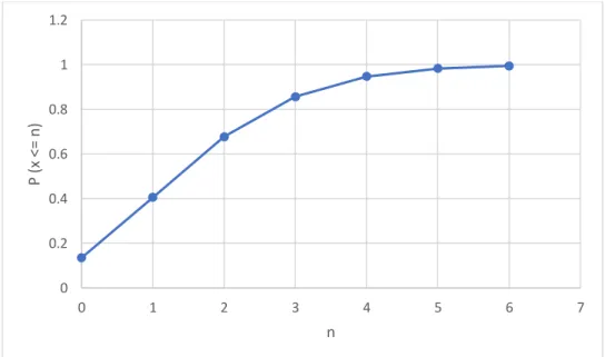
n P(n) P (x <= n) F(n) 0 0.135 0.135 8.120 1 0.271 0.406 16.240 2 0.271 0.677 16.240 3 0.180 0.857 10.827 4 0.090 0.947 5.413 5 0.036 0.983 2.165 6 0.012 0.995 0.722

Table 2 Probability values of vehicle arrivals computed using Poisson distribution

The probability that the number of vehicles arriving is between 2 to 4 is given as: p(2 ≤ x ≤ 4) =

p(2) + p(3) + p(4) = .271 + .18 + .09 = 0.54.

For more clearance the Figure 4 shows the Probability values of vehicle arrivals computed using Poisson distribution, and Figure 5 is drawing the cumulative probability values of vehicle arrivals computed using Poisson distribution.

Page | 12

Figure 4 Probability values of vehicle arrivals computed using Poisson distribution

Figure 5 Cumulative probability values of vehicle arrivals computed using Poisson distribution

3.1.2 Birth and death transitions processes (Markov chains)

When population is the number of customers in the system, λn and µn indicate that the arrival and service rates depend on the number in the system. Based on the properties of the Poisson process, i.e. when arrivals are in a Poisson process and service times are exponential, we can make the following probability statements for a transition during (t, t + ∆t) [41].

The birth-death process is a special case of continuous time Markov process [40] [42] [43], where the states (for example) represent a current size of a population and the transitions are limited to birth and death. When a birth occurs, the process goes from state i to state i + 1. Similarly, when death occurs, the process goes from state i to state i − 1. It is assumed that the birth and death events are independent of each other.

0 0.05 0.1 0.15 0.2 0.25 0.3 0 1 2 3 4 5 6 7 P (n) n 0 0.2 0.4 0.6 0.8 1 1.2 0 1 2 3 4 5 6 7 P ( x <= n) n

Page | 13 The Markov process refers to a discrete state which can be enumerated with k=0,1, 2,…etc, the state transitions occurs between the neighbouring states only i to i+1 or i to i-1, the BD process can be as its explained in Figure 6 [40].

Figure 6 Birth and death processes Markov chains [42]

The birth rate {λi}i=0,1,2,….,∞. probability of birth in interval ∆t is λi∆t.

The death rate {μi}i=0,1,2,….,∞. probability of death in interval ∆t is µi∆t.

In each state the probability of having birth and death would be calculated in the way described below [39]: Pk+1 and someone leaves the system is equal to the percentage of time for state Pk and someone arrive to system

Pi+1(death i+1) = Pi (birth i)

From Figure 6 the probability equations will be concluded to each state Determine P1 0=-λ0P0+μ1P1 Since P0 equal to 0 P1 = λ0 μ1 𝑃0 Equation 8 For P2 0 = −(λ1 + µ1) P1 + λ0P0 + µ2P2

Replacing the value of P1 that we have from Equation8. 0 = −(λ1 + µ1) λ0 μ1 𝑃0 + λ0P0 + µ2P2 Simplifying it more 0 = −λ1 λ0 μ1 𝑃0 − µ1 λ0 μ1 𝑃0 + λ0P0 + µ2P2 0 = −λ1 λ0 μ1 𝑃0 − λ0 𝑃0 + λ0P0 + µ2P2

Page | 14 0= −λ1 λ0 μ1 𝑃0 + µ2P2 P2= λ0λ1 μ2μ1 P0 Equation 9

Same procedure will be used for P3, P4, …. etc now we have

P1 = λ0 μ1 𝑃0 P2 = λ0λ1 μ1μ2 𝑃0 P3 = λ0λ1λ2 μ1μ2μ3 𝑃0 P4 = λ0λ1λ2λ3 μ1μ2μ3μ4 𝑃0 P𝑛 = λ0λ1…λ(𝑛−1) μ1….μ𝑛 𝑃0

Page | 15

3.1.3 Queuing theories

We faced queues many times during our normal day, just like when somebody going to bank to draw or deposit money, he have to wait in a queue in order to be served by the service desk, people who arrive earliest have to be served first that kind of queues and serving system called (FIFS first in first served), if there were only one service desk the queuing and serving process will be classified as M/M/1 in general we can identify having one arrival and one server at a time can be modelled as an M/M/1 queuing system, if the servers were two then the modelling will be M/M/2, if they are three then M/M/3 and so on. In our case we will study the M/M/1 and M/M/2.

3.1.3.1 (M/M/1)

M/M/1 is the most widely used queuing systems in analysis as pretty much everything is known about it. M/M/1 is a good approximation for many queuing systems [44] [40]. The arrivals are assumed to occur in a Poisson process with rate λ. This means that the number of customers N(t) arriving during a time interval (0, t) has a Poisson distribution, mentioned in section (3.1.1). Combined with section (0) with Pn(0) = 1 when n and i are equal to zero. For a complete solution of these difference–differential equations the use of generating functions (to transform the difference equation) and Laplace transforms (to transform the differential equation) is needed. Because of the complexity of the procedure and the result, we do not provide it in this text. Interested readers may refer to chapter 4 in [45] book where the results have been derived in detail.

In our case of study Intersections and how to model the traffic will be as follows:

μ: the service rate in Figure 7 is presented as the service agencies.

λ: Arrival rate is the rate of costumers arrive to intersection; we assume here that arrivals arrive randomly. ρ: arrivals rate / service rate.

Since the μ must be equal to λ so the system is stable, thus we get

𝜌 =𝜆

𝜇 The traffic intensity or utilization coefficient [41] Equation 10

The number of arrivals in the intersection system (N) can be calculated by 𝑁 = 𝜌

1−𝜌 Equation 11

or 𝑁 = 𝜆

𝜇−𝜆 Equation 12

Page | 16 Number of arrivals waiting for service (waiting in queue) it also called queue length

𝐿𝑞 =

𝑝2

1−𝑝 Equation 13

It also can be written as: 𝐿𝑞=

𝜆2

𝜇(𝜇−𝜆) Equation 14

Total (mean) waiting time (including the service time) 𝑇 =𝑁 𝜆 ➔ 𝑇 = 𝜌 𝜆(1−𝜌) ➔ = 1 𝜇(1−𝜌) ➔ = 1 𝜇−𝜆 Equation 15

Waiting time in queue exclude service time

𝑇 = 𝜌

𝜇(1−𝜌) or it can be written as 𝑇 =

𝜆

𝜇(𝜇−𝜆) Equation 16

Since the system will be using later is M/M/1 queuing system, thus λ0 = λ1 = λ2 = λ3 = λ4 = λn , same case with μ0 = μ1 = μ2 = μ3 = μ4 = μn P1 = λ μ 𝑃0 P2 = λ^2 μ^2 𝑃0 P3 = λ^3 μ^3 𝑃0 P4 = λ^4 μ^4 𝑃0

And to determine how the state probabilities evolve as a function of time π(t) we take the derivation:

ⅆ ⅆ𝑡

𝑝(𝑡) = 𝑝(𝑡) ⋅ 𝑄

To find the Q value we use the linear matrices

𝑄 =

(

0

…

…

𝜇

(

)

0

…

0

(

)

0

⁞

0

(

)

⁞

⁞

0

(

))

Page | 17

3.1.3.2 (M/M/2)

Same as M/M/1 we explain before in chapter 3.1.3.1 with a small difference, which is the arrivals are one and the servers are two, in case of performance measures that mean:

•

•

•

Equation 19

•

Equation 20

•

Equation 21

•

Page | 18

3.2 Difference among AV, CAV and Conventional Vehicles in an

intersection.

In this section we will highlight the main differences between the AV and the normal vehicles in an intersection. By Adding autonomous vehicles functionality to the traffic, at this stage we will study the autonomous vehicles properties and what is the main differences between the autonomous vehicles and the conventional vehicles when it comes to intersections. Also, we utilize technology approach in order to reduce the traffic congestion in an intersection.

There are two main communication for AV in intersections, and they are as follows:

Figure 8 Vehicular communication systems

3.2.1 The V2V communication

Vehicle to vehicle or V2V Communication is technological innovation. It allows two vehicles to ‘talk’ or ‘communicate’ with each other. It is also known as ‘V2X’. With the help of this technology, a vehicle can connect to the other nearby vehicles and supporting infrastructure.

For any Vehicle to Vehicle/V2V Communication system, there are two important factors 1. The communicating vehicle(s).

2. The roadside infrastructure with which the communication takes place [28].

3.2.1.1 V2V Data Processing

In order to enable the simplest collision prevention functionality, V2V technology requires a computer to process the data and generate driver alerts. For every additional application implemented, a more powerful computer is required. Computer devices that support V2V communication are rugged and capable of tolerating a broad range of operating temperatures. For example, an Axiomtek PICO880 [46] can function well in this environment as a V2V computer.

Similar to how a LiDAR computer system calculates the distance to detected objects for autonomous vehicles, a V2V computer system works to calculate the probability of impediments to alert drivers. In addition to driver

Page | 19 safety, using the data collected would make it easier to manage construction traffic and detours by guiding drivers to avoid obstacles. The computer is also used to facilitate passenger communication.

The actual communication takes place with the help of ‘Dedicated Short Range Communication (DSRC)’ wireless communication devices. As per the regulation in the United States, these devices work in the 5.9GHz band with a bandwidth of 75MHz which it separately assigned for the vehicular communication only. The approximate range of these devices is 1000m. DSRC devices communicate not only with the other vehicles but also with the road infrastructure [47].

In addition, when the vehicles equipped with V2V communication come in the connecting range of each other, they exchange information. It includes the position, speed, the direction of travel. It also informs the steering inputs being given by the driver and sudden change in driving conditions such as braking or lane change.

Since we are going to use the V2V technology in our simulation, more explanation and algorithm explaining will be in the chapter 3.3.2.1).

3.2.2 V2I communication (Vehicle to Infrastructure)

• Vehicles that enter the cooperative area notify the intersection controller with their presence.

• The intersection controller maintains a priority graph (for admitted vehicles) and a waiting list for non-admitted vehicles. The controller works in discrete time. At each time step, one or several vehicles will be admitted and assigned with priorities according to a priority assignment policy. Such policy can be adapted from the polling system.

• Admitted vehicles can autonomously cross the intersection under the assigned policy. Non-admitted vehicles are required to avoid entering the intersection area.

• Once vehicles leave the intersection, they are removed from priority graph and the corresponding priority relations are revoked [12].

More details of the V2I is explained in Algorithim1 , Flowchart in Figure 9 and Figure 10.

Algorithm 1

---

The vehicle to infrastructure algorithm. Vehicle V sends a message to infrastructure, which responds according to policy P.

1: loop

2: receive message from V 3: if message type is Request then

4: process request for new reservation with P 5: if P accepts the request then

Page | 20 7: else

8: send Reject message to V

9: else if message type is Change-Request then 10: process request for change of reservation with P 11: if P accepts the request then

12: send Confirm message to V containing the reservation returned by P 13: else

14: send Reject message to V

15: else if message type is Cancel then 16: process cancel with P

17: send Acknowledge message to V 18: else if message type is Done then 19: record any statistics supplied in message 20: process cancel with P

21: send Acknowledge message to V

Figure 9 V2I and I2V Flowchart

Page | 21

Figure 10 V2I Communication in an intersection

The above presented framework requires strong assumption: perception is perfect, communication is without delay, control is simple and there are only automated vehicles with the same dynamics and obeying the rules. There are many possibilities of failures in both perception and control. One can consider a perception failure as an unexpected event when the information arrives too late with respect to a normal functioning.

3.2.3 The Connected Autonomous Vehicles (CAV)

They are the kind of vehicles who have the both two technologies (V2V & V2I) we explain in previous subchapters (3.2.1 & 3.2.2).

It is important to note, however, the difference between AVs. CAVs can communicate with each other in what we call V2V and with roadside units (RSUs), traffic control signals and other infrastructure or devices. Ultimately, the vehicle is part of an intelligent transport system (or ITS) where all vehicles and infrastructure systems are connected, allowing for traffic information to be widely available to aid in optimization and increased security, reduce congestion, fuel consumption, etc... However, itis important to note that CAVs can be autonomous and not require a human driver in transit.

The Cooperative adaptive cruise control CACC [48] is one emerging technology application with the potential to enhance mobility on freeways. CACC aims to reduce gaps between communicating CAVs, facilitating the creation of tightly spaced vehicle platoons. V2V communication enables the precise transmission of position,

Page | 22 steering, acceleration, braking and other operating characteristics of other vehicles in the platoon, enabling safe and reliable platoon formulation.

Page | 23

3.3 Modeling and simulation

In this study the software Live PTV Vissim [49] [37] will be used as a simulator. We contact the PTV company and ask to provide us a special licence for thesis research, and they send it to us.

The reason of choosing Vissim because it is a user friendly and for simplicity reasons like: • Primarily it is easy to code using Python programming language.

• Provides numerous calibration parameters that could be modified. • the results displayed in real time on the software GUI.

• The results saved automatically on SQL database file after each simulation which make it easier for the us to analyse and save for further comparison.

The parameters that will be considered in the simulation are congestions (Queue length), fuel consumptions, waiting time and level of service (LOS), the level of service is a qualitative measure used to relate the quality of traffic service. LOS is used to analyse highways by categorizing traffic flow and assigning quality levels of traffic based on performance measure like speed, density, delay etc [50] and it mark from A to F in a way that A is excellent, B is very good, C is good, D is average, E is ok, and F mean failed or bad quality.

3.3.1 Simulation environment setup

The first step of developing the VISSIM model was to draw the network. Second, traffic volume for each direction were allocated to each lane group. The Wiedemann 74 car-following model was used because it was recommended by PTV Group to be used in traffic The car following model considers the changes in vehicle speeds in response to the performance of those vehicles immediately in front, The car following model is one of three primary equations applied during the simulation of a VISSIM model. The other two models include the lane change algorithm which is applied to assess upcoming opportunities and requirements to change lanes for each vehicle, as well as a route choice algorithm to determine the origin-destination path building process [51]. The model incorporates changes in driver conditions from free flow speeds to congested networks. In addition, the traffic volume also included 2% heavy vehicles on all approaches. Third, signal timing was coded in the VISSIM simulation model according to the field signal timing data. Last, conflict areas and priority rules were needed in the simulation model to simulate the vehicle movements more appropriately. Regarding the Driving Behaviour signal control, the Conventional vehicles use reaction time distribution no. 2 (2s ± 0.3s), AV-cars do not use any distribution.

The speed limit to be set to 50 km/h during simulation. The simulator models an area that is 250 m × 250 m. The intersection is located at the center of that area, and its size is determined by the number of lanes traveling in each direction, which is variable. We assume throughout that vehicles drive on two lanes the first one goes forward and to the right side of the road, the second one goes only in one way to the left as it explained in Figure 3.

Page | 24

3.3.2 Simulation Experiment

Here pseudo code for AV and CAV will be included.

3.3.2.1 For AV pseudo code

1. Initial V2V vehicle has no message 2. Initial V2V vehicle has message 3. Initial the distance between each vehicle 4. Assign threshold Distance

5. Assign speed 6. Start

7. Check if there are any vehicles in the network. 8. For (all number of vehicles (Get attributes))

9. Reading the world coordinates (x y z) for all vehicles and save them in list. 10. Read destination vehicle speed, position, acceleration

11. If (distance between destination vehicle and vehicle follow < threshold Distance) 12. Set (attribute vehicle follow = attribute destitution vehicle)

13. Assign vehicle follow to destination vehicle

Do the same procedure for all vehicles in the network respectively. (By sending message from one to the next one).

Page | 25

Figure 11 (AV algorithm flowchart)

3.3.2.2 For CAV pseudo code

The procedure is same as Pseudo code for AV vehicles (3.3.2.1) the difference is the CAV is equipped with technology that enable it to communicate with the traffic light, The vehicle can check the traffic light if its green or red, according to the feedback the vehicle is adjusting the speed and acceleration.

The code to be added is:

• If (traficGreen and minimum speed)

minimum speed is required to arrive during the current green. if (the desired speed is higher than the minimum speed)

Page | 26 else minimize the speed until it gets less than the desired speed

• If (traficGreen and maximum speed)

The vehicle should not drive above the maximum speed in order to arrive just when the next green starts. if (the maximum speed is higher than the desired speed)

keep desired speed because the desired speed to lower than the maximum speed => the vehicle will arrive after the signal turned green

For (all vehicles (Get attributes))

• keep speed a little smaller so that vehicle arrive shortly before the signal head. • read vehicle attributes

• if there are any vehicles in the network

• Maximum speed to arrive at the next green start. If the vehicle drives faster, it would arrive at the signal before the next green time.

• Minimum speed to arrive at the next green end. If the vehicle drives slower, it would not make it in the current / next green time.

• if the original desired speed has not yet saved, save it

• if the vehicle does not have an upcoming signal: set original desired speed • jump to next vehicle

To have the optimal the speed with respect to traffic lights:

• If minimum speed for arriving before the next green end is higher than the maximum speed to arriving after the next green start. This is only possible in case the next signal is green.

• Set the speed to the optimal speed. • Else

• Go to minimum speed with respective to the destination vehicle.

3.3.3 Traffic distribution in intersection

To give the best results a comparison has been made among the (Conventional vehicles, AV, CAV and last a combination of AV and CAV).

Good to note that the Connected Autonomous Vehicles (CAVs) receive the information about the upcoming signal and adjust their speed to arrive at green without stopping.

On a four-arm intersection, from each direction the identical volume approaches the intersection but in different vehicle compositions, this four-arm intersection has been done to distinguish the differences in the chapter results.

• West entry: conventional vehicles with the PTV Vissim default driving parameters without the ability to receive the signal information.

• North entry: autonomous vehicles (AVs) with adjusted driving parameters (e.g. smaller safety distance) but no ability to receive the signal information.

Page | 27 • East entry: a mix of autonomous vehicles (AVs) as described in North entry and Connected

Autonomous Vehicles(CAVs) with adjusted driving parameters (e.g. smaller safety distance) and the ability to receive the signal information.

• South entry: Connected Autonomous Vehicles(CAVs) with adjusted driving parameters (e.g. smaller safety distance) and the ability to receive the signal information.

Connected vehicles receive the information about the time until the next green start and next green end from the signal. Together with the current distance from the vehicle to the signal, the optimal speed for arriving at the next green start and end is calculated.

Figure 12 Traffic modelling

Vehicles in the simulator have the following properties: • Vehicle Identification Number (VIN)

• Length • Width

• Distance from front of vehicle to front axle • Distance from front of vehicle to rear axle • Maximum velocity

• Maximum acceleration • Minimum acceleration • Maximum steering angle • Sensor range (for AVs, CAVs) And the following state variables:

Page | 28 • Position • Velocity • Heading • Acceleration • Steering angle

4 Results

In this chapter a total result will be listed for the project work.

4.1 Results RQ1

The important result coming out of the analysis states are:

1. The departure process of the M/M/1 queue in equilibrium is the same Poisson as the arrival process. Consequently, the expected number of customers served during a length of time t when the system is in equilibrium is given by λt. Likely the customers who has been already served in the same time are μt. 2. Also, in method we describe how to calculate the traffic utilization ρ, the expected queue length Lq and the

expected waiting time T to be served.

3. We could address the probability of each state p(0), p(1), p(2)…. p(n). that make the relationship between each neighbour states easy to calculate.

4. By using method from section 3.1.1 for any state we have in section 3.1.2, we can solve the queue length and the waiting time in stops at any case in section 3.1.3.

4.2 Results RQ2

Reduced traffic congestion

In AV the collisions are avoided because of the vehicle’s communications in other word all the vehicles are cooperated in the intersection. And that leads to the deadlock is autonomously controlled. Under normal circumstances, human drivers naturally create stop-and-go traffic, even in the absence of bottlenecks, lane changes, merges or other disruptions, by controlling the pace of the autonomous vehicle in the study, they were able to smooth out the traffic flow for all the vehicles.

CAVs have the potential to increase efficiency on intersections, arterials and surface streets through reducing vehicle headways when platooning, operating with traffic signals, utilizing intelligent merging with automated on-ramp metering, and harmonizing speeds to smooth traffic flow (reduce waiting time in intersections). Additionally, with fewer crashes anticipated due to safety improvements, non-recurring congestion stemming from crashes should fall.

Page | 29

4.3 Results RQ3

4.3.1 Detailed statistical results

In this section we will list the detailed results for all vehicles trajectory grouped by their type Conventional, AV, the mix of AV & CAV, and CAV.

Conventional vehicles come from Western side as it has been explained in Figure 12. Goes to three directions North, South and East (forward). The (LOS) has “F, E, E” marks in each direction respectively, and it has attributes as follows:

Figure 13 Conventional vehicles results detail

296 134 157 64.68 _{57.37 58.38 57.37 56.28 57.37} 11.527 _{4.917 5.505} 0 50 100 150 200 250 300 350 W-N W-E W-S

Conventional vehicles

Page | 30 Autonomous vehicles come from Northern side as it has been explained in Figure 12. Goes to three directions West, East and South (forward). The (LOS) has “C, C, C” marks in each direction respectively, and it has attributes as follows:

Figure 14 AV results detail

A mix between AVs and CAVs come from Eastern side as it has been explained in Figure 12. Goes to three directions West (forward), North and South. The (LOS) has “B, B, B” marks in each direction respectively, and it has attributes as follows:

Figure 15Mix of AV and CAV results detail

134 326 136 17.9 _13.68 19.41 _13.68 19.457944_13.68 2.45 6.28 2.59 0 50 100 150 200 250 300 350 N-W N-E N-S

Autonomous Vehciles

Number of vehicles Stop delay Queue length Fuel Consumption [US liquid gallon]

296 134 157 64.68 _{57.37 58.38 57.37 56.28 57.37} 11.527 _{4.917 5.505} 0 50 100 150 200 250 300 350

E-W E-N E-S

Mix of AV and CAV

Page | 31 Connected Autonomous Vehiclescomes from Eastern side as it has been explained in Figure 12. Goes to three directions West, North (forward), and East. The (LOS) has “A, A, B” marks in each direction respectively, and it has attributes as follows:

Figure 16CAV results detail

315 135 141 3.2 4.95 3.92 1.51 4.95 1.57 3.62 4.95 1.8 0 50 100 150 200 250 300 350 S-W S-N S-E

Connected Autonomous Vehicles

Page | 32

4.3.2 Results Comparison

This section represents the comparison based on results we have from previous sub chapter (4.3.1), first for the M/M/1 queuing system

Vehicle type Level of service Number of Vehicles Stop Delay (In sec) Queue Length (m) Fuel Consumption [US liquid gallon]

Conventional F 296 64.68 57.37 11.52

AV C 326 19.41 13.68 6.28

AV & CAV B 290 7.00 6.03 4.46

CAV A 315 3.20 4.95 3.92

Table 3 M/M/1 Queue comparison

And for the M/M/2 queuing system:

Vehicle type Level of service Number of Vehicles Stop Delay (In sec) Queue Length (m) Fuel Consumption [US liquid gallon]

Conventional E 291 57.33 57.37 10.41

AV C 270 18.675 13.68 5.04

AV & CAV B 291 5. 21 6.03 4

CAV A, B 276 2.565 4.95 3.37

Table 4M/M/2 Queue comparison

Here we include a full detailed table for all types of vehicles and their trajectory.

Vehicle direction Level of service Number of Vehicles Stop Delay (In sec) Queue Length (m) Fuel Consumption [US liquid gallon]

W-N F 296 64.68 57.37 11.52 W-E E 134 58.38 57.37 4.91 W-S E 157 56.28 57.37 5.50 N-W C 134 17.90 13.68 2.45 N-E C 326 19.41 13.68 6.28 N-S C 136 19.45 13.68 2.59 E-W B 149 5.39 6.03 2.08 E-N B 142 5.03 6.03 1.92 E-S B 290 7.00 6.03 4.46 S-W A 315 3.20 4.95 3.92 S-N A 135 1.51 4.95 1.57 S-E B 141 3.62 4.95 1.80 Total C 2355 22.28 20.51 48.63

Page | 33 Finally, the final comparison among the vehicle types and their attributes

Vehicle type Level of service Number of Vehicles Stop Delay (In sec) Queue Length (m) Fuel Consumption [US liquid gallon]

Conventional F 587 179.34 57.37 21.93

AV C 596 56.76 13.68 11.32

AV & CAV B 581 17.42 6.03 8.46

CAV A, B 591 8.33 4.95 7.29

Table 6 Final comparison

Figure 17 Final Comparison

0 20 40 60 80 100 120 140 160 180 200

Stop Delay (In sec) Queue Length (m) Fuel Consumption [US liquid gallon]

Final Comparison

Page | 34

5 Discussion

In (V2I communication 3.2.2) There are many possibilities of failures in both perception and control. One can consider a perception failure as an unexpected event when the information arrives too late with respect to a normal functioning. The approach is not to fail silently but to have degraded control modes for which either the vehicle can still exit the intersection or can get a higher priority so that other vehicles let this failing vehicle leave the intersection (before stopping safely). Again, this can be handled as a kind of unexpected event leading to brake to keep brake-safe property.

5.1 Observations from results

As it shows in the final results the number of vehicles was almost the same from all directions (581-596), the only thing differ is their type attributes, the stop delay was extremely decreased from the conventional vehicles to the CAVs (179.34 sec to only 8.33 sec, 95.4% reduced) the reason back to the CAVs properties that they can communicate with each other’s and has the ability to make a platoon therefore the fuel consumption was 67% less also the communication between the vehicle and the infrastructure prevent the congestion as it shows the total amount of queues decreases significantly from (57.37m to 4.95m), while the conventional vehicles can have some interruptions like (human beings mistakes, and the safety distance between each vehicle.

The AVs was doing good so far with the results compared with the normal vehicles, but when it comes to the stop delay (waiting time) it can be easily notice that its relatively high compared with other attributes and that is because of the AVs missing the ability to communicate with the infrastructure (V2I, I2V) technology. Therefor there were a relatively long waiting time at the traffic lights compared with the CAVs, at CAVs the delay is reduced by 86%, naturally that effect on the queue length and fuel consumption.

5.2 Future Work

The study was considered successful but has several limitations making it difficult to generalise the findings. The results were therefore considered promising, but in need of further investigation.

This work can be further improved by:

• Consider more attributes for every vehicle type.

• Use (dummy vehicles) in simulations and compare it with simulator results.

• Develop the V2I and V2V communications algorithm in a way to present results that is closely the real world.

Page | 35

6 Conclusion

Connected Autonomous Vehicles will become a reality soon, our traditional traffic light intersections will become outdated and the need to develop more efficient automated intersections will be possible. Both the communication among vehicles to other vehicles and vehicles to the infrastructure will be needed.

To summarize the work, we did in this project, for the first research question, we performed literary research about the traffic modelling, we use the Poisson distribution to generate a discrete arrival to the system, those arrivals combined with the birth-death processes we use them as an input for M/M/1 & M/M/2 queueing system. We find the relation among the (waiting time, queue length for each state, traffic utilization, fuel consumption) in discrete time interval. The analysis and simulations are based on results from queueing theory, an area of mathematical analysis that relies heavily on the theory of Markov processes. Specifically, a bottleneck is modelled as a node in a network of servers and road users arriving at intersections are modelled as customers joining the queue of the server.

Second research question we did a wide research has been done on the autonomous vehicles a comparison among them has been made based on their kind of communications, the first was a normal autonomous vehicles (uses V2V technology), second was a Connected Autonomous Vehicles(which has the ability to communicate with the infrastructure, uses the V2V, V2I and I2V technology), third is a mix between the AV and CAV, last a normal conventional vehicles used in the comparison process, to highlight the advantages of the new technology used in CAV.

Third research question we answer it by simulations of the algorithm show that the minimizing total delay algorithm can also minimize the total number of stops, and hence, is more suitable for implementation. The results of this work show promise for reducing traffic congestion at intersections by deploying the next generation of Connected Autonomous Vehicles since the delay was reduced to only 4.6% and the vehicles queue 8.62% compared to the normal conventional vehicles, we use now days.

Page | 36

7 References

[1] K. K. Daniel J. Fagnant, “Preparing a nation for autonomous vehicles: opportunities,barriers and policy recommendations,” Transportation Research Part A, vol. 77, pp. 167-181, 2015.

[2] “https://searchenterpriseai.techtarget.com,” [Online]. Available:

https://searchenterpriseai.techtarget.com/definition/driverless-car. [Accessed 29 07 2019].

[3] G. N. Aashiq Parker, “How to best Automate Intersection Management,” in 2017 IEEE Congress on

Evolutionary Computation (CEC), San Sebastian, Spain, 5-8 June 2017.

[4] J. L. C. L. Elnaz Namazi, “Intelligent Intersection Management Systems Considering Autonomous Vehicles: A Systematic Literature Review”. IEEE Access, Vol. 7, pp. 91946-91965, 2019.

[5] M. Rouse, “intelligent transportation system,” 03 2017. [Online]. Available: https://whatis.techtarget.com/definition/intelligent-transportation-system. [Accessed 30 07 2019]. [6] “https://stattrek.com,” [Online]. Available: https://stattrek.com/probability-distributions/poisson.aspx. [7] I. B. Dr. Tom V. Mathew, “Vehicle Arrival Models : Count,” 19 February 2014. [Online]. Available:

https://nptel.ac.in/courses/105101008/downloads/cete_13.pdf.

[8] C. O. O. a. E. O. Otumba, “Modelling of Distribution of the “Matatu” Traffic Flow Using Poisson Distribution in a Highway in Kenya,” International Mathematical Forum, vol. 13, pp. 385 - 392, 2018. [9] “https://www.onallcylinders.com,” Google, [Online]. Available:

https://www.onallcylinders.com/wp-content/uploads/2017/09/07/Waymo-Self-Driving-Car.png. [Accessed 29 07 2019].

[10] J. C. S. a. D. C. Chin, “Traffic-responsive signal timing for system-wide traffic control,” Transportation

Research Part C: Emerging, vol. 5, p. 153–163, 1997.

[11] U. D. o. Transportation, “National Agenda for Intersection Safety.,” Federal Highway Administration, Washington, 2005.

[12] X. Q. Arnaud de La Fortelle, “Autonomous driving at intersections: combining theoretical,” in ITS

World Congress 2015, ERTICO - ITS Europe, Bordeaux, France., Oct 2015.

[13] H. K. ANDRÉ JOSEFSSON, “Intersection Control for Autonomous Cars through a Reservation Scheme,” Degree Project in Computer Science, DD143X, Project thesis in Computer Science, DD143X, 11 05 2016.

[14] E. Djuana, “Analysis and Design of Traffic Lights Control System by Design and Analysis of Real-Time Systems (DARTS) Methodology,” Trisakti University, Jakarta, Indinosea, 2005.

[15] K. R. F. G. S. T. R. R. D. A. E Djuana*, “Simulating and evaluating an adaptive and integrated traffic lights control system for smart city application,” International Seminar on Sustainable Urban

Development , pp. 1-6, 2018.

[16] SG Colaco, CP Kurian, VI George and AM Colaco, “Integrated design and real-time implementation of an adaptive, predictive light controller,” Lighting Res. Technol, p. 459–476, 2012.

[17] P. Mingola, “A Study of Poisson and Related Processes with Applications,” University of Tennessee , Tennessee , 2013.

[18] M. Hosamo, “A Study of the Source Traffic GeneratorUsing Poisson Distribution for ABR Service,”

Modelling and Simulation in Engineering, vol. 2012, p. 6, 18 June 2012.

[19] A. G. K. H. K. J. D. T. Raimund Bürger, “Difference schemes, entropy solutions, and speedup impulse for an inhomogeneous kinematic traffic flow model,” American institute of mathmatical science, 2008. [20] H. R. Ismail H. Zohdy, “Game theory algorithm for intersection-based cooperative adaptive cruise

control (CACC) systems,” in Conference on Intelligent Transportation Systems, Anchorage, AK, USA, 2012.

[21] J. I. Hoffman, Biostatistics for Medical and Biomedical Practitioners, Germany, 2015, pp. 259-278. [22] B. A.-G. Anas Al-Roubaiey, “Coverage Optimization of Wireless Sensor Networks with Normal

Distribution,” in Acronym: ICIS, Dhahran, 31261, Saudi Arabia, 2018. [23] The normal distribution.. [Film]. Austiralia : University of Melbourne, 2017.

Page | 37 [24] S. M. L. &. D. R. Jeske, “Some Suggestions for Teaching About Normal Approximations to Poisson

and Binomial Distribution Functions,” The American Statistician, p. 8, 2009.

[25] S. V. U. Feng Zhu, “A linear programming formulation for autonomous intersection control within a dynamic traffic assignment and connected vehicle environment,” Transportation Research Part C, no. 55, p. 363–378, 2015.

[26] K. Dresner and P. Stone, “Multiagent Traffic Management: A Reservation-Based Intersection Control Mechanism,” in The Third International Joint Conference on Autonomous Agents and Multiagent

Systems, New York, USA, July 2004.

[27] K. Dresner and P. Stone, “Human-Usable and Emergency Vehicle–Aware Control Policies for Autonomous Intersection Management,” in The Fourth Workshop on Agents in Traffic and

Transportation (ATT 06), Hakodate, Japan, May 2006.

[28] K. Dresner and P. Stone, “Sharing the road: autonomous vehicles meet human drivers,” Vols. Austin, Texas 78712-0233, pp. 1263-1268, 2007.

[29] P. S. Tsz-Chiu Au, “Motion planning algorithms for autonomous intersection management,”

AAAIWS'10-01 Proceedings of the 1st AAAI Conference on Bridging the Gap Between Task and Motion Planning, pp. 2-9 , 2010.

[30] J. Lebacque, “Intersection Modeling, Application to Macroscopic Network Traffic Flow Models and Traffic Management,” Traffic and Granular Flow ’03, pp. 261-278, 2005.

[31] M. J. L. a. G. B. Whitham, “theory of traffic flow on long crowded roads, In Proceedings of the Royal Society of London,” Mathematical, Physical and Engineering Sciences, vol. 299, pp. 317-345, 1955. [32] S. P. H. a. P. H. Bovy, “State-of-the-art of vehicular traffic flow modelling,” Systems and Control

Engineering, no. 215, p. 283{303, 2001.

[33] “https://www.aimsun.com/,” Siemens, [Online]. Available: https://www.aimsun.com/.

[34] “https://www.trafficware.com/synchro.html,” Trafficware, [Online]. Available: https://www.trafficware.com.

[35] S. N. R. a. T. R. Institute, “https://www.vti.se/en/,” Swedish National Road and Transport Research Institute, [Online]. Available: https://www.vti.se/en/.

[36] M. N. Akililu, “Verification of Rural Traffic Simulator, RuTSim 2,” Linköpings universitet,

Institutionen för teknik och naturvetenskap, Kommunikations- och transportsystem. Linköpings universitet, Tekniska högskolan, p. 79, 2012.

[37] “http://vision-traffic.ptvgroup.com/en-us/products/ptv-vissim/,” PTV Group, [Online]. Available: http://vision-traffic.ptvgroup.com/.

[38] “https://sumo.dlr.de,” [Online]. Available: https://sumo.dlr.de/wiki/Simulation_of_Urban_MObility_-_Wiki.

[39] J. Julvez, “http://www.suaybarslan.com,” [Online]. Available:

http://www.suaybarslan.com/birthdeathprocess4datamodelling.pdf.

[40] S. G. H. d. M. K. S. T. Gunter Bolch, Queueing Networks and Markov Chains, New Jersey: A JOHN WILEY & SONS, INC, 2006.

[41] H. X. Y. Z. Baoqun Duan, “Queuing system performance analysis and Markov control process(M),”

Hefei: the press of University of science and technology of China, 2004.

[42] “Wikipedia,” 21 Jan 2019. [Online]. Available:

https://en.wikipedia.org/wiki/Birth%E2%80%93death_process.

[43] A. Mitrofanova, “Lecture 3: Continuous times Markov chains.Poisson Process.Birth and Death process.,” NYU, department of Computer Science, NewYork, December 18, 2007.

[44] A. A.-A. K. A. F. T. O. Martin Anokye, “Application of Queuing Theory to Vehicular Traffic at Signalized Intersection in Kumasi-Ashanti Region, Ghana,” American International Journal of

Contemporary Research, vol. 3, no. 7, July 2013.

[45] U. N. Bhat, “Simple Markovian Queueing Systems,” Dallas, Texas, Southern Methodist University, pp. 75-93.