Wind resource assessment comparison on a complex terrain employing WindPRO and WindSim

(1)

THESIS BY

NIKOLAOS SIMISIROGLOU

Submitted to the Office of Graduate Studies of Gotland University

in partial fulfillment of the requirements for the degree of WIND POWER PROJECT MANAGEMENT

Approved by:

Supervisor, Bahri Uzunoglu

Examiner, Jens Nørkær Sørensen

June 2012

(2)

ABSTRACT

Wind resource assessment comparison on a complex terrain employing WindPRO and WindSim.

(June 2012)

Nikolaos Simisiroglou, BSc in Physics, University of Crete Supervisor: Dr. Bahri Uzunoglu

Accurate wind resource assessment is of high importance for wind farm development. This thesis estimates and compares the annual energy production results produced employing two wind farm design tools WindPRO and WindSim for a site located in Greece.

Two years of data are available from a 56 meter met mast. The data are analyzed filtered and converted to appropriate formats for usage by the wind farm design tools. Abnormalities in the wind data are observed, investigated and presented.

For energy calculations in WindPRO different roughness data and height contours are used and evaluated resulting to 36 different energy estimations. The result show that the annual energy production results for different parameters have a difference from 0,07% to 8,18 %. Concerning energy estimations using WindSim a grid sensitivity study is produced utilizing a low resolution grid to an ever more refined grid for

different boundary layer heights and air density’s.

Parameters introducing uncertainties and energy losses in the calculations are identified and quantified. Using the annual energy production, uncertainty and energy losses the P50, P75, P90 are produced for WindPRO, WindSim and are compared. These result indicate a good approximation in the estimated values from both wind farm design tools, for the investigated site the result differences vary from 0,2 % - 2,0%.

(3)

(4)

ACKNOWLEDGEMENTS

This thesis would not have been possible without the support of numerous people. Firstly I would like to thank my Supervisor, Dr. Bahri Uzunoglu for his valuable guidance and time. Thanks, as well to Richard Koehler, Dr. Stephan Ivanell, Liselotte Alden and the entire Wind Power Project Management (WPPM) faculty of Gotland University for their support in numerous issues. Continuing, I would like to thank the PROTERGIA family, especially Yiannis Tsagarakos, Kuriakos Berdebes, Maria Beskou, Xenophon Karamitsos and all the gentleman of room 303A for their warm welcome, assistance and provision of the necessary resources for the completion of this project. Furthermore, thanks to Li Di of the WindSim support team for his precious help. I would like thanks and express my sincere gratitude and appreciation to Katerina Mouzouraki, my family and numerous friends for their support and presence. Finally, from the depths of my heart I would like to thank Melissanthi Mavridou for her patience and love.

(5)

NOMENCLATURE

AEP Annual Energy Production

CORINE 2000 Coordinated Information on the European Environment Valley

CFD Computational Fluid Dynamics

EIA Environmental Impact Assessment

MCP Measure Correlate Predict

NCAR National Center for Atmospheric Research

RANS Reynolds Averaged Navier Stokes

SRTM Shuttle Radar Topographic Mission

(6)

LIST OF FIGURES

Page Figure 1: Wind profiles for different surfaces. From left to right the wind profiles

indicate a rough surface (high friction) to a smooth surface (lower friction). Source

(Earnest & Wizelius, 2011) ... 12

Figure 2: View towards the Northern direction ... 15

Figure 3: Mean wind speed data removed for the 56m anemometer... 18

Figure 4: Mean wind speed data removed for 28.5m, 31.8m, 38.5m, 41.0m, 53.5m anemometers ... 18

Figure 5: Availability for anemometer at 56m ... 19

Figure 6: Gun shot diagram 56.0m - 53.5m ... 20

Figure 7: General xy graph of mean wind speed values for 56.0m and 53.5m ... 20

Figure 8: Weibull distribution’s for 56.0m, 53.5, 28.5m ... 21

Figure 9: Monthly wind speed means from 23/10/2009-22/10/2011 for all heights ... 22

Figure 10: Monthly mean wind speed for 23/10/2009-23/10/2010, first year (previous page) and 23/10/2010-22/10/2011, second year (present page) ... 23

Figure 11: Turbulence intensity per sector and wind speed ... 24

Figure 12: Main enabled wind statistics for 22/11/2010-22/10/2011 ... 24

Figure 13: Wind frequency and energy rose ... 25

Figure 14: Correlation of wine vanes at 53.5m and 31.8 m ... 26

Figure 15: Mean monthly temperatures in Celsius ... 27

Figure 16: Terrain steepness presentation ... 28

Figure 17: Roughness length areas ... 29

(9)

Figure 19: Wind farm layout, height contours and roughness lines ... 31

Figure 20: Grid refinement for 1 500 000 cells ... 33

Figure 21: Particle tracing for wind field from NNW direction ... 34

Figure 22 : Turbulence intensity cut plane for the NNW sector ... 34

Figure 23: Wind resource of 1 500 000 cells case with a height of boundary layer equal to 500 and air density of 1,184 for heights of 55m (left) and 78m (right) ... 35

(10)

LIST OF TABLES

Page

Table 1: Basic technical parameters and mounting of met mast ... 16

Table 2: Wind shear per sector ... 21

Table 3: Weibull A and k parameters and wind direction percentage of occurrence per sector ... 26

Table 4: AEP differences for varying time series ... 31

Table 5: Distribution of the first 10 nodes in z-direction ... 32

Table 6: Grid size in xy direction ... 33

Table 7: Properties of energy module ... 35

Table 8: WindSim parameter AEP % differences for 1 500 000 ... 36

Table 9: Estimation of Energy Losses ... 37

Table 10: Estimation of Total Uncertainty ... 39

(11)

CHAPTER I

INTRODUCTION AND LITERATURE REVIEW

1.1 Introduction

For the successful development of wind energy sites a project manager must investigate apart from the wind energy resource available on site other factors such as proximity to electrical grid, support mechanism, land ownership, conflicting interests, local acceptance, planning restraints and other (Earnest & Wizelius, 2011).

Nevertheless, wind energy resource is a crucial if not the most important component for identifying promising sites for wind farm development. For this reason wind resources maps have been made in many countries during the last decade at national and regional levels with the purpose to identify possible areas apt for wind energy development; an example of such a case is the wind resource map of Europe by Risø National Laboratory (Troen & Petersen, 1989). These maps, however useful, have usually a low resolution and should be used solely for identifying possible sites of interest. As will be seen further in the text, local conditions influence greatly the wind condition at the site of interest making micro-siting necessary for accurate prediction of the local wind resource. Assessing wind resources for micro-sitting, meaning using short term measurements to identify long term wind resources, wind speeds, wind profile, wind distribution, turbulence etc. for energy projects is not a trivial issue. For such purposes a number of data acquisition techniques and wind resource assessment models have been developed by numerous institutes and companies (Probst &

Cárdenas, 2010).

In this study we will estimate and compare the annual energy production results produced employing two WFDT (wind farm design tools), namely WindPRO and WindSim for a site situated on a complex terrain in Greece. Furthermore for each WFDT the influence of certain parameters on the AEP estimation will be investigated for the site of interest. The wind data for the study will be provided by in situ

measurements using a 56 m height met mast consisting of two years of data

measurements. The study will present a methodology for analyzing wind data, AEP percentages differences will be presented for different parameters such as roughness, height contours, height of boundary layer etc. The selected AEP results produced from WindPRO and WindSim will further be compared for the following cases GROSS AEP, AEP including wake effects, P50, P75 and P90.

1.2 Literature review

In this section we will present the basic characteristics of the wind such as the wind profile and turbulence, local impacts influencing the wind as roughness, obstacles and orography and relevant factors as internal boundary layer, long term correlation and the Weibull distribution. Furthermore, the technical basics of energy calculation models used in WindPRO and WindSim will be displayed.

(12)

1.2.1 Wind Characteristics

Winds are driven by the sun. The solar radiation heats parts of Earth’s surface differently because of its round shape, rotation around its axis, surface material etc. causing temperature differences that in turn cause atmospheric pressure differences. Winds are the movements of air that tend to equalize these pressure differences. The air mass movements are a combination of five different forces; gravitational force, pressure gradient force, Coriolis force, centrifugal force and friction force (Ackerman & J.A.Knox, 2003). Close to the Earth the wind is influenced by friction against the surface. The friction force acts against the air movement creating a wind profile (Figure 1). For the first tens of meters in the atmosphere the wind profile varies greatly with height depending on the type of surface.

Figure 1: Wind profiles for different surfaces. From left to right the wind profiles indicate a rough surface (high friction) to a smooth surface (lower friction). Source (Earnest & Wizelius,

2011)

The two main models attempting to capture this variation are the power law and the logarithmic profile:

Power law

Logarithmic profile Where: Uz the wind speed at height z

Ur the wind speed at a reference height r

α the wind shear exponent u* the friction velocity

κ the von-Karman constant equal to 0.4 z0 the roughness length

There are rather high discrepancies between these two models according to some researches; a wind speed extrapolated to other heights employing the power law or the logarithmic profile might have discrepancies in the vicinity of 10% depending on surface roughness and height of extrapolation (Sørensen & J.N.Søresen, 2011). The height where the wind speed is no longer influenced by the surface roughness is named gradient height; further, the wind at that height is called geostrophic wind.

(13)

When the movement of the wind is parallel to the surface the wind flow is called laminar, alternatively when the movement is in other direction around the prevailing wind, moving in eddies and waves then the flow is turbulent (Earnest & Wizelius, 2011). Turbulence may be caused by obstacles in the flow, orography or temperature differences in the air and it appears as short variations of wind speed. An approach to quantify the turbulence is by statistical means using the dimensionless measure named turbulence intensity, I, defined as (Stull, 2009)

Whereas, is the standard deviation around the mean wind speed .

On a local level the wind is influenced among others by terrain roughness, obstacles and orography. The terrain is classified in five different roughness classes; although usually for calculation, the parameter used is the roughness length z0 that

indicates how the terrain influences the wind speed. As wind moves over different terrain roughness internal boundary layers appear changing the wind profile; however after a while the internal boundary layer stabilizes, until the surface roughness

changes again that in turn will cause the profile to change as well (Earnest & Wizelius, 2011). Locally, obstacles e.g. building in the terrain may cause relative speed decreases in the wind speed, vertically up to three times the height of the obstacle and downstream to 30-40 times the height (Troen & Petersen, 1989). As for the orography depending on the steepness, wind speed roughness and other, it may influence the wind speed in many ways, such as; the speed might increase up slope and decrease down the slope afterwards if the slope of the hill is smooth and not to steep. However if the orography is complex then the flow might become turbulent and lead to an opposite effect, meaning a decrease in wind speed.

Long term correlation of wind data may be achieved by statistical methods such as the MCP method, as will be seen long term correlation is critical for accurate AEP estimations of a wind farm for a life span of 20 years. The reason for this is that the wind resource varies from year to year in our case more than 12% and from one decade to another up to 30% (Troen & Petersen, 1989).

The frequency distribution of wind speeds is approximated by the two parameter Weibull distribution, where f(u) is the frequency of occurrence and is defined as:

1.2.2 Wind Farm Design Tools review

The models used for calculating wind recourses are usually divided into

Analytical and Numerical models. In this study an analytical model such as WAsP, the model employed by WindPRO for AEP calculation will be compared with

WindSim a numerical model. WAsP is a linear model developed by Risø laboratories in Denmark, published in 1989 while the pc model was publicly available one year later. The model takes into account per sector:

(14)

a) The geostrophic balance. Where the geostrophic wind is given by the geostrophic drag law , G is the

geostrophic wind, f the Coriolis parameter, and A and B are dimensionless functions of stability (for neutral conditions, A = 1,8, B = 4,5).

b) The logarithmic wind profile. where u*

is the friction velocity, k the von Karman constant (≈0,4), z0 the roughness length, and ψ the

stability dependent function, positive for unstable conditions and negative for stable conditions.

c) –A specific (but uniform) stability. d) –Roughness variations.

e) –Height variations

The PARK module in WindPRO utilizes WAsP and additionally contains several different wake loss models and advanced turbulence calculations facilities for wind farm AEP calculations. Detailed information may be found in (Troen &

Petersen, 1989) (EMD, n.d.)

On the other hand the numerical model WindSim is a CFD tool based on the 3D Reynolds Averaged Navier Stokes (RANS) solver. The non-linear transport

equations for mass, momentum and energy are solved employing Phoenics as a computational engine. Different turbulent closures are available by WindSim; in this report the two parameter k-e model will be used. WindSim is a suitable tool for simulations in complex terrain, and in situations with complex local climatology. Assessment of wind resources is accomplished with both experimental and numerical means. The numerical model calculates the terrain-induced acceleration of the wind field, the so-called speed-up. The model takes into account:

a) The geostrophic balance. b) The logarithmic wind profile. c) A specific (but uniform) stability. d) Roughness variations.

e) Height variations.

f) Turbulence (nonlinear effects).

Furthermore WindSim is dependent on resolution it is as well time consuming and requires a rather high level of experience since there are many possible adjustments within the model. More information concerning WindSim methodologies may be found at (WindSim, n.d.).

(15)

CHAPTER II

DATA ANALYSIS

2.1 Site Description

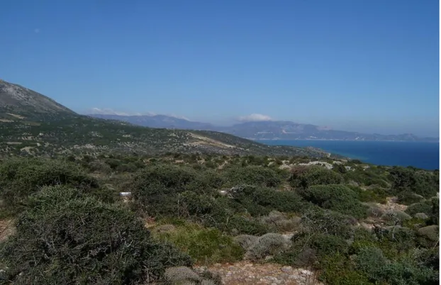
The under investigation site is situated on a complex terrain in Greece that is characterized by mountains with significant differences in height. The area confined for the wind park has an altitude variation of roughly 61 – 194 meters located on bare hills with small vegetation like grass and bush land (Appendix A). Surrounding the location of interest from the north-northeast to the southern direction is the sea, at approximately one kilometer distance. In the western direction there is a sharp mountain range stretching at a length of two kilometers from the site (Figure 2).

Figure 2: View towards the NNW direction

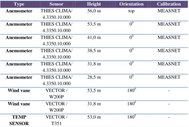
A 54 meter met mast was adopted for onsite data acquisition. The met mast consists of 6 wind anemometers at different heights, two wind vanes and a thermometer (Table1). Two years of wind speed, wind direction and temperature data are available since 2009. In the following pages, the data will be analyzed and filtered using

(16)

Type Sensor Height Orientation Calibration

Anemometer THIES CLIMA/ 4.3350.10.000

56,0 m top MEASNET

53,5 m 00 MEASNET

41,0 m 00 MEASNET

38,5 m 00 MEASNET

31,8 m 00 MEASNET

28,5 m 00 MEASNET

Wind vane VECTOR / W200P

53,5 m 1800 -

Wind vane VECTOR / W200P 31,8 m 1800 - TEMP SENSOR VECTOR / T351 53,0 m 1800 -

Table 1: Basic technical parameters and mounting of met mast

2.2 Wind speed data

The wind speed data consist of a two year time series taken at ten minute time intervals. Minimum, maximum, average and standard deviation values are recorded for heights of 28,5m, 31,8m, 38,5m, 41,0m, 53,5m, 56m. Throughout the text the anemometers will be referred as the “56m anemometer or 53,5m anemometer” in place of the “anemometer at a height of 56m a.g.l” for simplification reasons. For data collection, Thies Clima wind anemometers were used and installed in the northern direction of the met mast, an exception to this is the anemometer installed at the top of the met mast at a height of 56m; all anemometers are calibrated according to

MEASNET cup anemometer calibration procedure 09/1997 and have accordingly the appropriate certificate for use in wind speed data acquisition.

2.2.1 Analysis of wind speed data using WindPRO

Using the WindPRO meteo object to produce a time series, data from each anemometer is imported into WindPRO as a .tab file. The produced time series subsequently will be inspected and analyzed thoroughly in the following pages. Data quality checks are performed for all measurements, accordingly to standard practice amongst others to the following criterions:

(17)

 Rejection of periods in which anemometers did not send signal (frozen sensors, defected sensors).

 Rejection of periods in which vanes sent continuously the same signal (frozen sensors, defected sensors).

 Rejection of measurements (velocity, direction) which deviate highly from the general trend of concurrent measurement with other sensors with good

correlation coefficient.

 Rejection of velocities lower than the expected value (ratio check) due to shadow effects from the masts, booms, wires, appearance of other sensors or obstacles in the mast etc.

The graphics that will be employed for the analysis are:

 Time series; for identifying efficiently corrupted and erroneous data and further enabling and disabling data.

 Weibull; for plotting the Weibull distribution for different heights.  Gun shot diagram; for data correlation, evaluation of tower shadowing in

different directions and data abnormalities.

 General X-Y graph; for identifying abnormal data.

 Profile; for identifying the wind profile and shear exponent for all sectors. While the statistics that will be used are:

 Main statistics.  Monthly means.  Availability.

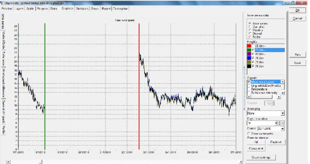
Starting, each anemometer was investigated separately for possible areas of corrupted data using the time series graphics. For the 56m height anemometer, data from 15/12/2009 at 18:20 until 03/06/2010 15:10 are disabled because they are corrupted (Figure 3).

(18)

Figure 3: Mean wind speed data removed for the 56m anemometer

The data are identified as corrupted because the logger installed on the met mast recorded for 6 months starting on the 15/12/2009 at 18:20, continues wind speed values of 0,258 m/s, equal to the anemometers offset. To present, the reason for the anemometers malfunction has not been registered; though according to the weather report on the day of the malfunction there was heavy rain with lightning in the area of the site (Arniakos, n.d.). This observation leads us to speculate that a high voltage charge was probably the cause for the malfunction.

Looking into the time series of the 28,5m, 31,8m, 38,5m, 41,0m, 53,5m anemometers, we are able to determine data from 15/12/2009 at 18:20 until 15/12/2009 at 23:50 and data from 18/01/2010 16:50 until 22/01/2010 12:50 as corrupted and are disabled (Figure 4). Up to date no specific information is available concerning the reason leading to the data corruption.

(19)

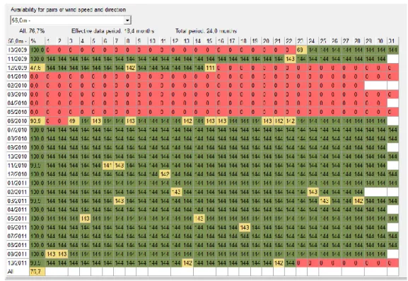
Concerning the availability of data, for the anemometer situated at 56 m height the availability reaches 76.7% (Figure 5) while for the other heights the availabilities are 99.3 %.

Figure 5: Availability for anemometer at 56m

Continuing the analysis, wind speed differences between different heights are investigated. A total of fifteen different combinations are plotted in a gun shot

diagram, an example is shown in Figure 6. From Figure 6 one is able to distinguish that the data is protruding outwardly in the South SSE direction. This bulge is apparent from the gun shot diagrams where data from any anemometer is subtracted from the data of the anemometer located at 56m height. A possible reason for this is tower shadowing (Saba, 2002) (Orlando, et al., 2010). In more detail, all anemometers with the exception of the anemometer at 56m are installed in the northern direction of the met mast, while the anemometer at 56m is located on top of the met mast; thus when the wind direction is from the south all anemometers are shaded with an exception for the anemometer at 56m. This observation leads us to speculate that tower shading is apparent for all anemometers except the anemometer situated at 56 m, making the usage of that anemometers wind data critical for the avoidance of introducing a high level of uncertainty in the energy calculations made in Chapter III. However, since there is 6 months of corrupted data for the 56 m height anemometer the remaining 18 month time series is further cut down to 12 months for the

avoidance of seasonal bias in our calculations.

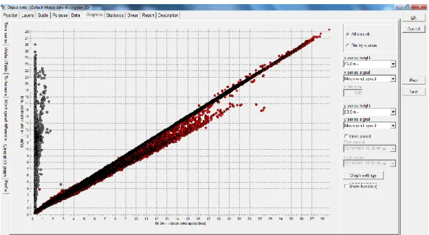
Next fifteen different combinations of general xy graphs of mean wind speed values for different heights are plotted and examined (Figure 7).

(20)

Figure 6: Gun shot diagram 56.0m - 53.5m

Figure 7: General xy graph of mean wind speed values for 56.0m and 53.5m From the general xy graph we have that data with the largest deviation appeared when comparing wind speeds from the 56m anemometer with the other anemometers. Data retaining the largest discrepancies were recorded on the 11/12/2010, the reason for this is not yet clarified. However, from the temperature recorded on the specific date we are able to observe that the temperature is between 00C and -1 0C, indicating that there might be icing issues present on the top

anemometer causing the apparent deviation of wind speeds.

As for the wind shear per sector, under the profile tab in graphics, WindPRO estimates among others the wind shear profile; the values calculated per sector are presented in Table 2:

(21)

Sector Power law exponent Average 0,040 N 0,028 NNE 0,045 ENE 0,060 E 0,080 ESE 0,000 SSE 0,025 S 0,186 SSW 0,140 WSW 0,121 W 0,097 WNW 0,048 NNW 0,012

Table 2: Wind shear per sector

The Weibull distribution graphs are plotted for three different heights as shown in Figure 8. It is observed that there is a smooth fit of the Weibull distribution to the wind speed distribution with no apparent abrupt changes.

Figure 8: Weibull distribution’s for 56.0m, 53.5, 28.5m

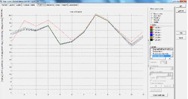
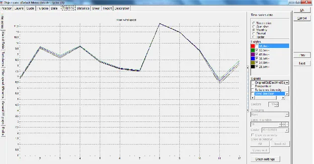
The monthly mean wind speeds for all anemometer heights are shown in Figure 9 for wind speed data from 23/10/2009 until 22/10/2011.

(22)

Figure 9: Monthly wind speed means from 23/10/2009-22/10/2011 for all heights Observing Figure 9 one is able to distinguish an anomaly in the correlation of the 56m anemometer in comparison with the other five anemometers for the first 6 months of the plot. This anomaly is attributed to the missing 6 months of data for the anemometer at 56m height. Following, the monthly mean wind speeds are plotted for two different years. The first year consists of data from 23/10/2009 until 23/10/2010 and the second year consists of data starting 23/10/2010 ending 22/10/2011(Figure 10).

(23)

Figure 10: Monthly mean wind speed for 23/10/2009-23/10/2010, first year (previous page) and 23/10/2010-22/10/2011, second year (present page)

One is able to observe from Figure 10 how well correlated the data are and the different monthly wind profiles for the site; these profiles are typical for Greece, having a maximum in August.

The percentage of yearly variation using data from the anemometer located at 53,5m is calculated by the following equation:

Where : mean wind speed for the first year 23/10/2009 until 23/10/2010

: mean wind speed for the second year 23/10/2010 until 22/10/2011 The local yearly variation is 12,5%; this value indicates that a long term correlation using MCP methods is of high importance for an accurate average annual energy estimation of the next twenty year period. The estimation of the local yearly variation was accomplished using the anemometer located at 53,5m instead of the 56m height anemometer because of the high availability of data reaching up to 99,3% ,whereas the anemometer at 56m is missing approximately 6 months of measurement for the first year.

Hereafter data from the second year will be used throughout the document unless indicated otherwise for calculations, meaning data from 23/10/2010 to

22/10/2011. By averaging the ten minute wind speed data and standard deviation the turbulence intensity for the anemometer at 56m height is calculated for each sector and wind speed, accordingly to the following equation (Figure 11):

(24)

Where TI: average for all speeds turbulence intensity : ten minute interval average standard deviation : ten minute interval average means wind speed

Figure 11: Turbulence intensity per sector and wind speed

The turbulence intensity per wind speed and sector is rather low as seen in Figure 11. By averaging for all sectors and wind speed we obtain a value for

turbulence intensity in the vicinity of 0,1, indicating a fairly laminar flow over the site of interest.

Finally, by using the statistics tab in WindPRO the main enabled statistics are shown and presented in Figure 12. The Weibull mean speeds are higher for the anemometer located at 56m decreasing steadily towards the anemometer located at 28.5 m as expected. This confirms that the anemometers are placed in the right sequence from the technicians that installed the met mast.

(25)

2.2.2 MCP analysis

For MCP analysis four NCAR data sets provided by the WindPRO database are used. The maximum correlation coefficient result achieved between the 56 m anemometer correlating with each of the four NCAR data sets is 0,632 , this result was achieved by using different filters and averaging methods provided by the MCP module. The result from the correlation is considered of poor quality (Nielsen, 2010). Therefore, long term correlation using MCP methods is not conducted in our study since other sources of long term data were not available.

Looking into the reason for the low correlation coefficient result and what affects this result, one could argue that there might be time delays between weather patterns arriving at the two sites since the minimum distance between the site and the NCAR data is about 139 km away, unique weather patterns, topographic effects that create unique flow patterns at one site or the other. (Manwell, et al., 2002)

2.3 Analysis of wind direction data using WindPRO

Similarly, two years of direction data comprising of the minimum, maximum, average and standard deviation was recorded and acquired from the two

Vector/W200P wind vanes at heights of 53,5m and 31,8m respectively. This data is then imported into WindPRO. From the wind rose (Figure 13) it is observed that the main wind direction is NNW followed by north and finally south.

Figure 13: Wind frequency and energy rose

The wind speed for the NNW is higher for the season of summer followed by spring, autumn and winter. For Northern direction the wind speed is higher for the season of spring followed by winter, autumn and summer. While in the Southern direction the wind speed is higher in autumn followed by winter, spring and summer. For NNW and Southern direction the daytime speed profiles are higher than the night time for all season in contrast with the Northern direction where we have higher

(26)

speeds in the night time for spring, autumn and winter. Figure 14 presents the correlation graph of the two wind vanes at height of 53.5m and 31.8m respectively; one is able to observe that the wind vanes are fairly correlated

Figure 14: Correlation of wine vanes at 53.5m and 31.8 m

In addition Table 3 presents the wind direction percentage of occurrence for each direction and the Weibull A and k parameter for each sector at a height of 56 m. All calculations for the wind speeds at the height of 56,0m and 53,5m are utilizing the data from the wind vane at 53,5m while the anemometers at heights 41,0, 38,5, 31,8, 28,5 are utilizing the data from the wind vane at 31,8m.

(27)

2.4 Analysis of Temperature

The overall climatic conditions in this area can be described as a summer-dry, sub-tropic or Mediterranean. Two years of data is available from the thermometer installed at a height of 53.0m on the met mast. This data is imported to WindPRO and

analyzed. Data from 15/12/2009 at 18:20 until 15/12/2009 at 23:50 and data from 18/01/2010 16:50 until 22/01/2010 12:50 are removed because they are corrupted. The temperature is generally over 0 oC with an exception of 2 days where the

temperature drops to a minimum of -1.3 oC. This indicates that there will be no icing issues considering the site. The monthly mean temperature values are shown in Figure 15.

Figure 15: Mean monthly temperatures in Celsius

2.5 Height contours

Height contours were provided using SRTM satellite data, the format was given in .dat. The file had three columns that contained xyz coordinates with a minimum resolution of 15m. This was then converted to .xyz file format and imported to WindPRO. The xyz points then were converted and edited using a time consuming process to height contours employing the EMD editor that is available from

WindPRO. For comparison height contours are downloaded from the database incorporated into WindPRO, the height contours have a height separation of 5m and comprise an area of more than 20km x 25km. Both height contour maps are compared with a high precision topographic map 1:50000 acquired from the Greek military. From this investigation it was concluded that height contours from the database of WindPRO will be used for the final energy estimation in the Chapter III. The reason for this is that the height contours from WindPRO are found to represent the

orography of the site more accurately. Following, terrain steepness calculations are performed.

(28)

Figure 16: Terrain steepness presentation

The steepness in the direct surrounding area of the wind farm is calculated up to 30 degrees as shown in Figure 16, indicating the complexity of the terrain. These results for terrain inclination indicate that the site is at the limit of the accuracy of the WAsP software, making the use of a CFD tool compelling.

2.6 Roughness

Roughness data were obtained from CORINE 2000 (Coordinated Information on the European Environment) satellite gained data base, aerial photos and topographical maps. The total area of the applied roughness map comprises an area of more than 20 km x 30 km (Figure 17). The under investigation roughness area was downloaded to a .dwg file and then converted to .dxf and imported to WindPRO using the Insert area data icon. This was compared with the online databases of WindPRO.

(29)

Figure 17: Roughness length areas

To determine which roughness database represents our site more accurately an onsite investigation was issued. This investigation determined that the roughness lines obtained from CORINE 2000 represent our site with higher accuracy and will be used for the final energy calculations.

CHAPTER III

ENERGY ANALYSIS

3.1 Wind farm layout

The wind farm consists of six Enercon wind turbines located in two groups. The first group consists of four E-82 E2 2300 wind turbines at 78m hub height and the second group comprises of two E-44 900 wind turbines at 55m hub height. The total capacity of the farm is 11 MW; the layout is shown in Figure 18. The power curves used for energy estimations and the thrust coefficient utilized for wake effect determination of both wind turbine types are given from the manufacturer for air densities of 1,225 kg/m3 and 1,18 kg/m3

(30)

Figure 18: Wind farm layout. Source: Google earth

3.2 Energy calculation using WindPRO

The wind data used for energy calculation is from the 56m anemometer for a time period of 23/10/2010-22/10/2011 and the wind vane at 53.5m height. Employing the WindPRO module Statgen, wind statistics of the site are produced and will be used for energy estimations. For energy calculations the Park module provided by WindPRO will be used and thirty six energy calculations (Appendix B) will be performed and compared employing different combinations described below:

a) Two wake models; N.O. Jensen (RISO/EMD) and Eddy Viscosity.

b) Three roughness lines; CORINE 2000, and two online databases provided from WindPRO, specifically the DataForWind: European Roughness Contour Data Based from www.DataForWind.com- 200 m grid and Modis VCF: Modis Vegetation Continuous Field Roughnesses- 500 m grid. c) Two height contours; WindPRO database and SRTM satellite data. d) Three wake model parameters based on terrain type; open farmland, mixed

farmland and closed farmland.

From the energy calculations the results demonstrate that the energy differences for different wake models are approximately 0,7 %, while for the

individual height contours the differences are 0,2 %, further for different wake model parameters based on terrain type the difference is in the vicinity of 0,08 % and finally for different roughness lines the energy difference reach up to 7,3 %. The largest

difference is observed when comparing the cases:

10a) Wake model Eddy Viscosity, 200 m grid roughness, open farmland, WindPRO heights contours

13b) Wake model Jensen, 200 + 500 m grid roughness, open farmland, satellite data height contours

(31)

The AEP% difference is 8,18% with the value from case 10a) higher then case 13b).

We must point out here that for all calculation a hub height of 78m was employed for key results. The air density used for the above energy calculations is estimated employing the climate data from the Athinai observatory. As for the power curves of each individual wind turbine, they have been adapted to the estimated air density at each turbine position automatically by WindPRO.

Figure 19: Wind farm layout, height contours and roughness lines

Furthermore AEP calculations are performed and compared for the 53,5m anemometer utilizing the full two year time series, the first year

(23/10/2009-23/10/2010) and second year (23/10/2010-22/10/2011) time series. The park module is employed with the following parameters; open farmland, height contours from the WindPRO database, CORINE 2000 roughness lines and N.O. Jensen wake module. The results utilizing equation

are shown in Table 4.

2nd year data for 56m anemometer

2nd year data for 53,5m anemometer

1st year of data for 53,5m anemometer

Two full years of data for 53,5m

anemometer

2nd year data for 56m anemometer

0 -2,1% -23,4% -11,8%

2nd year data for 53,5m anemometer

0 -20,9% -9,6%

1st year of data for 53,5m anemometer

0 9,4%

Two full years of data for 53,5m anemometer

0

(32)

As could be observed in Table 4 there is a 20,9% difference in the estimated AEP using the second year versus the first year data for the 53,5 m a.g.l. anemometer. This clearly shows how important long term correlation of wind data is for accurate estimation of the AEP. By comparing the AEP of the 2nd year time series data for both 56m and 53,5m a.g.l. anemometers a rough estimation of the order of magnitude of error from tower shadowing may be derived. The AEP estimation error from tower shadowing using the 53,5m a.g.l. is approximately -2,1%.

The results from the park module using open farmland, WindPRO database, height contours, CORINE 2000 roughness lines and N.O. Jensen wake model will be used in the following for comparison with the results obtained from the WindSim calculation.

3.3 Energy calculation using WindSim

As in WindPRO the wind data used for energy calculation in WindSim are from the 56m anemometer for the time period of 23/10/2010-22/10/2011 and the wind vane at the height of 53.5m. Height contour and roughness lines are imported in .map file and are converted to .gws by the convert terrain module incorporated into

WindSim. Following a grid sensitivity analysis will be performed along with the methodology used for each module in WindSim.

3.3.1 Terrain module

A total area of more than 14km x 16km is selected for the analysis; the refinement type is changed from no refinement to refinement area with a ratio additive length to resolution of 0,5. The cells in the z direction are set to 23, further the 3D grid is orthogonalized and the maximum number of cells will vary for the grid sensitivity analysis to be performed. The applied cases are 10 000, 20 000, 50 000, 100 000, 500 000, 1 000 000 and 1 500 000 cells are investigated. For all cases in z-direction the grid extends to approximately 2927,6 m above the point in the terrain with the highest elevation (Figure 20). The distributions of the first 10 nodes in z-direction are refined towards the ground (Table 5).

1 2 3 4 5 6 7 8 9 10 z dist. max (m) z dist. min (m) 11,5 12,5 39,4 49,3 76,6 96,0 123,4 154,6 179,5 224,9 245,2 307,2 320,2 401,2 404,8 507,1 498,7 624,8 602,1 754,4

Table 5: Distribution of the first 10 nodes in z-direction

Contrasting the grid size in the z direction, the min and maximum grid size in xy-direction varies depending on the maximum number of cells defined in the

(33)

Max. number of cells

x y z total

10 000 Grid min- max (m) 553,4-1513,5 390,1-1124,0 Variable -

Number of cells 16 27 23 9936

Number of cells 126 172 23 498456

1 000 000 Grid min- max (m) 22,1-406,5 22,3-263,4 Variable -

Number of cells 180 241 23 997740

1 500 000 Grid min- max (m) 17,9–311,5 17,9–234,4 Variable -

Number of cells 226 288 23 1497024

Table 6: Grid size in xy direction

Figure 20: Grid refinement for 1 500 000 cells

3.3.2 Wind Fields module

The wind field module will be run for two air densities 1,184 and 1,225 kg/m3 and two heights of boundary layer 500 and 1000m. The number of iterations is set to 400, however for sectors that more iteration is needed for convergence to occur they are performed. In addition the turbulence model used is the standard k-epsilon, whilst the solver is set to the coupled, an algebraic multi-grid solver which solves

(34)

Figure 21: Particle tracing for wind field from NNW direction

3.3.3 Objects module

The two groups, total of six wind turbines are imported to WindSim, the power curves used for each wind turbine are adapted to the air density used in the wind field module, for air density of 1,225 and 1,184 kg/m3 power curves of 1,225 and 1,184 kg/m3 respectively are used. The climatology data are imported from WindPRO; this was achieved by creating a .wws file from the frequency table of the meteo object in WindPRO compatible with WindSim. Following the turbulence intensity, 3D wind speed of the wind turbines are investigated roughly using cut planes (Figure 22).

(35)

3.3.4 Wind Resources module

The wind resource module is used for heights of 50m and 78m.The properties used in the calculation are; wake model 1, 1:20 for wake rotor diameter, wake sector sub cycle is set to 10 and the multiple wake model is based on sum of squares. The results from the WindSim run containing 1 500 000 cells, height of boundary layer equal to 500 and air density of 1,184 is presented below for heights of 55m and 78m (Figure 23).

Figure 23: Wind resource of 1 500 000 cells case with a height of boundary layer equal to 500 and air density of 1,184 for heights of 55m (left) and 78m (right)

3.3.5 Energy module

The properties used for all the energy calculation are displayed in Table 7.

(36)

By refining the grid from 10 000 to 1 500 000 cells a grid independent solution was reached at 1 500 000. Figure 24 presents the AEP of the models, for height of boundary layer equal to 500 and air density of 1,184 against the number of cells used in the 3D models:

Figure 24: AEP against the number of cells in the 3D models

The AEP % differences utilizing equation 2 for 1 500 000 cells for different parameters are shown in Table 8:

Constant parameter Value Varying parameters Value AEP% difference

Air density 1,184 Boundary layer height

500 and 1000 0,15% Air density 1,225 Boundary layer

height

500 and 1000 0,14% Boundary layer

height

500 Air density 1,225 and 1,184 2,4% Boundary layer

height

1000 Air density 1,225 and 1,184 2,4%

Table 8: WindSim parameter AEP % differences for 1 500 000

AEP

(37)

CHAPTER IV

RESULTS

4.1 Energy Losses

Each action in the process of transforming the kinetic energy of the wind to electric energy in the grid inherently incubates a certain percentage of losses. The losses identified in our case are shown in Table 9 as a percentage of the total production.

Parameter Wind Pro Expected Losses WindSim Expected Losses

Wake effect Availability Turbine Performance Electrical Curtailment 1,5% 5% 1% n.a n.a 0,78% 5% 1% n.a n.a Total 7,5% 6,78%

Table 9: Estimation of Energy Losses

Each wind turbine creates a wake downwind of the rotor; the air in the wake in comparison with the free stream wind is more turbulent and transports less kinetic energy. Hence, in a wind farm wind turbines located downwind and in the wake of a wind turbine are affected negatively energy wise and produce less energy. To capture this phenomenon the N.O Jensen (RISO/EMD) wake model is used in WindPRO and wake module 1 is used in WindSim. The results of the estimated wake energy losses for our wind farm are:

WindPRO N.O Jensen (RISO/EMD) wake model: 1, 5% WindSim wake model 1: 0, 78 %

By availability we mean the total time the wind turbine is available for electricity generation. This value includes regular maintenances of the wind turbines, adequate reaction times of the service teams as well as adequate provision times for spare parts, substation availability and electric power grid fault that is external to the wind power facility. An availability of 95% is assumed, resulting to 5% availability energy losses.

The turbine performance energy losses include blade degradation, fouling high wind hysteresis and wind flow. Energy losses due to high wind hysteresis occur when the wind turbine is stopped for wind speeds under the cut out wind speed; the reason for this phenomenon is that the wind turbine does not resume immediately to normal operation mode when the wind speed decreases from the cut out to operating speed. The energy that is lost in this process has to be extracted manually. Wind flow losses are losses due to turbulence, off yaw axis winds, inclined flow and high wind shear. Thus it is estimated that turbine performance energy losses are approximately 1%. Electrical losses considering cables, wind turbine transformers, substations and

(38)

facility electrical needs are not possibly estimated to date for the site. The same applies for possible curtailment applied to the wind park; possible reasons for curtailment are derived from power purchase agreements, grid curtailment and ramp-rate, flickering, noise or environmental issues such as birds and bats.

4.2 Uncertainty analysis

It is commonly accepted that wind resource assessment is a time consuming process that is subject to a great deal uncertainty. The introduced uncertainties

correspond either to random error or systematic error and unknown bias. The first are produced by the variability of the quantity being measured and in the measurement procedure e.g. wind speed, the latter are generated constantly over a set of identical measurements as a result of for example error in calibration, physical models and so on. The following uncertainties have been identified for the site of interest:

 Wind related uncertainties

o Measurement Uncertainty: dynamic over speeding and cup anemometer calibration uncertainty, vertical flow effects, vertical turbulence effects 3%, Mounting tower effects boom 4%

o Data Processing; Data Analysis 2%, Long-term Correlation 0% since long term correlation was not performed

o Prediction Horizon 13%  Transfer to the Energy Level

o Modeling 10% o Air density 2% o Power curve 5%

4.2.1 Wind related uncertainties

The measurements uncertainties of wind speed are made by Thies clima/ 4.3350.10.000 anemometers calibrated according to MEASNET standards, which are state of art anemometers. For wind direction Vector/ W200P wind vanes are used, calibrated according to MEASNET standards. Thus, a total measurement uncertainty for dynamic over speeding, cup anemometer calibration, vertical flow effects, and vertical turbulence effects is estimated to 3%. Furthermore, mounting uncertainty, meaning influences to the measurements from the mast itself, booms and mounting clamps, are estimated to 4%.

Data processing uncertainty consist of uncertainties associated with data analysis and long term correlation. Data analysis uncertainties include; quality of the

(39)

Weibull fit to the actual wind frequency distribution, uncertainties introduced by data processing, removing corrupted data and data coverage. The total data analysis uncertainty is 2%. Long term correlation was not used in this project; hence the long term correlation introduced uncertainty is 0%.

The prediction horizon uncertainty which depends on year to year variability and future climate variability of the area is estimated to 13% (Kwon, 2009) (Lackner, et al., n.d.).

4.2.2 Transfer to energy level uncertainty

How wind related uncertainties transfer to energy level uncertainties through horizontal and vertical extrapolation is not a trivial issue. It would be wrong to estimate the energy uncertainty by the theoretical cubic relation of wind speed and energy. Therefore an estimated value of 10% is assigned to model uncertainty. The air density according to the ideal gas law is depended on the air temperature, air pressure and gas constant. Therefore the air density varies constantly for different time

periods. The air density uncertainty has been calculated to 2%. As for the power curve an uncertainty of 6% has been associated to it since the power curve is based on idealized wind conditions and a site specific measured power curve was not available (Kwon, 2009). The uncertainties in energy losses calculated in section 3.4 are

estimated to 3%.

4.2.3 Overall uncertainty

The values for wind speed and transfer energy uncertainties are approximate and generic (Table 10). The total uncertainty for one year is calculated using root sum square formula: Parameter Uncertainty Measurement Mounting Data analysis Long term correlation

Prediction horizon Model Air density Power curve Energy Losses 3% 4% 2% 0% 13% 10% 2% 6% 3% Total 18,6%

(40)

4.6 NET Energy

The NET energy production or P50 or central estimate is calculated based on the AEP GROSS energy production, the energy losses and uncertainties. The

assumption made is that the AEP follows the normal distribution and that all uncertainties used for the calculation are independent. Using the Loss&Uncertainty module in WindPRO and the values from Table 9 and 10 the P50, P84, P90 values are calculated for WindPRO. Similarly using the losses and uncertainty tool of WindSim and Table 9 and 10 the P50, P84, P90 values are calculated for WindSim. The

percentage differences in the results of WindPRO against WindSim are shown below:

AEP % difference between two models

GROSS AEP AEP including wake effects

P50 P75 P90 1,8% 1,0% 1,9% 0,2% 2,0%

Table 11: AEP percentage differences between the two models

CHAPTER V

DISCUSSION AND CONCLUSION

For this project one year of wind speed data was used from the 56m

anemometer for energy calculations even though two years of data was availabe from the other anemometer’s. The reason for this is that the one year of wind speed data retrieved from the 56m height anemometer was subject to minimum influence from the met mast in comparison to the other anemometers Figure 6. This incident, meaning that from a two year time series only one year of wind speed data is

appliable for energy calculation indicates how important is to install on either sides of the met mast anemometers to filter out shadowing effects if the top anemometer malfunctions. Specifically if at 53,5m a.g.l. two anemometer where instaled, one on either side of the met mast preferably to only one anemometer at 53,5 m a.g.l.; then it would be possible to filter out the shadowing effects caused by the met mast, making it possible to calculate the AEP of the site with greater accuracy using a two year time series rather then only one.

Energy estimation for wind power projects using only one year of wind speed data inherently have a high level of uncertainty because of year to year variation here 12,5% causing a AEP difference of 20,9 %, future climate changes and climatic variations that cannot be accurately predicted but are estimated to vary up to 30% (Troen & Petersen, 1989). Therefore, long term correlation is vital for accurate energy production estimations. In our case this was not possible since a long term time series of acceptable correlation coefficient was not found introducing a high uncertainty factor to our energy calculation, here estimated to 13% prediction horizon uncertainty. The wind rose for the site of interest has a typical shape for Greece,

(41)

where typicaly few sector have high percentages of occurency, here NNW, North and South.

Concerning the WindPRO AEP calculations it is obvious that the different height contours data, wake models and terrain type do not influence the AEP significantly in comparison to the roughness lines where a difference of more than 7,3% is apparent. For WindSim AEP calculations it is observed that the highest AEP percentage difference outcome is for different air densities up to 2,4% while for different heights of boundary layers the AEP % differences are up to 0,15%. For the vertical extrapolation from the top anemometer to hub height and the transfer of wind data from the measurement point to the turbine positions the Park model in WindPRO and the CFD-Model WindSim has been used a model uncertainty of 10% was

appointed to both models respectively. This value is generic since the Park and flow model uncertainties where not possibly determined by cross prediction checks

between measurement systems, since other measurement systems were not available.

Finally concerning the AEP differences of WindSim and WindPRO, the models forecasts differences for GROSS AEP, AEP including wake effects, P50 P75, P90 are in the vicinity of 1% (Table 11), this is considered a good correlation and might be attributed to the high proximity of the met mast and the under investigation wind farm layout. On the other hand the AEP uncertainty for both models is approximately 18,6% which is acknowledged as a high value for uncertainty.

Recommended future fields of study and investigation are:

 Investigating the difference in AEP if long term correlation of the wind speed measurements is used.

 Investigating how does the estimated AEP of the wind farm estimated by WindSim and WindPRO vary for different proximities from the met mast.  Investigating the presence of thermal winds affecting the wind farm

production and quantifying the level of the affect.

 Quantifying the shadow or speed up effects produced on the anemometers from the met mast with higher precision.

 Evaluating uncertainties and assigning values to each uncertainty by a more standardized and specific way.

 Further understanding of long term variability of wind resources and how climate change impacts the energy output of wind farms.

(42)

(43)

(44)

Appendix B

36 Cases are used for comparison:

1) Wake model Jensen, CORINE 2000 roughness, open farmland, 1a)WindPRO heights contours and 1b) satellite data height contours 2) Wake model Jensen, CORINE 2000 roughness, closed farmland,

2a)WindPRO heights contours and 2b) satellite data height contours 3) Wake model Jensen, CORINE 2000 roughness, mixed farmland

3a)WindPRO heights contours and 3b) satellite data height contours 4) Wake model Eddy Viscosity, CORINE 2000 roughness, open farmland,

4a)WindPRO heights contours and 4b) satellite data height contours 5) Wake model Eddy Viscosity, CORINE 2000 roughness, closed farmland,

5a)WindPRO heights contours and 5b) satellite data height contours 6) Wake model Eddy Viscosity, CORINE 2000 roughness, mixed farmland,

6a)WindPRO heights contours and 6b) satellite data height contours 7) Wake model Jensen, 200 m grid roughness, open farmland, 7a)WindPRO

heights contours and 7b) satellite data height contours

8) Wake model Jensen, 200 m grid roughness, closed farmland, 8a)WindPRO heights contours and 8b) satellite data height contours

9) Wake model Jensen, 200 m grid roughness, mixed farmland, 9a)WindPRO heights contours and 9b) satellite data height contours

10) Wake model Eddy Viscosity, 200 m grid roughness, open farmland, 10a)WindPRO heights contours and 10b) satellite data height contours 11) Wake model Eddy Viscosity, 200 m grid roughness, closed farmland, 11a)WindPRO heights contours and 11b) satellite data height contours 12) Wake model Eddy Viscosity, 200 m grid roughness, mixed farmland, 12a)WindPRO heights contours and 12b) satellite data height contours 13) Wake model Jensen, 200 + 500 m grid roughness, open farmland,

13a)WindPRO heights contours and 13b) satellite data height contours 14) Wake model Jensen, 200 + 500 m grid roughness, closed farmland,

14a)WindPRO heights contours and 14b) satellite data height contours 15) Wake model Jensen, 200 + 500 m grid roughness, mixed farmland,

15a)WindPRO heights contours and 15b) satellite data height contours 16) Wake model Eddy Viscosity, 200 + 500 m grid roughness, open farmland,

16a)WindPRO heights contours and 16b) satellite data height contours 17) Wake model Eddy Viscosity, 200 + 500 m grid roughness, closed farmland,

17a)WindPRO heights contours and 17b) satellite data height contours 18) Wake model Eddy Viscosity, 200 + 500 m grid roughness, mixed farmland,

(45)

The values are calculated from the equation below and are in percentage:

Example: The % difference of 1a and 1b is:

1a 1b 2a 2b 3a 3b 4a 4b 5a 5b 6a 6b 7a 1a 0,00 -0,23 0,09 -0,15 0,04 -0,19 0,52 0,29 0,52 0,29 0,52 0,29 2,46 1b 0,00 0,32 0,09 0,28 0,04 0,75 0,52 0,75 0,52 0,75 0,52 2,69 2a 0,00 -0,23 -0,05 -0,28 0,43 0,20 0,43 0,20 0,43 0,20 2,38 2b 0,00 0,19 -0,05 0,66 0,43 0,66 0,43 0,66 0,43 2,61 3a 0,00 -0,23 0,47 0,25 0,47 0,25 0,47 0,25 2,42 3b 0,00 0,71 0,48 0,71 0,48 0,71 0,48 2,65 4a 0,00 -0,23 0,00 -0,23 0,00 -0,23 1,96 4b 0,00 0,23 0,00 0,23 0,00 2,18 5a 0,00 -0,23 0,00 -0,23 1,96 5b 0,00 0,23 0,00 2,18 6a 0,00 -0,23 1,96 6b 0,00 2,18 7a 0,00 7b 8a 8b 9a 9b 10a 10b 11a 11b 12a 12b 13a 13b 14a 14b 15a 15b 16a 16b 17a 17b 18a 18b

(46)

8a 8b 9a 9b 10a 10b 11a 11b 12a 12b 1a 2,55 2,35 2,50 2,31 3,05 2,86 3,05 2,86 3,05 2,86 1b 2,77 2,58 2,73 2,53 3,27 3,09 3,27 3,09 3,27 3,09 2a 2,46 2,26 2,42 2,22 2,96 2,77 2,96 2,77 2,96 2,77 2b 2,69 2,49 2,64 2,45 3,19 3,00 3,19 3,00 3,19 3,00 3a 2,50 2,31 2,46 2,26 3,00 2,82 3,00 2,82 3,00 2,82 3b 2,73 2,54 2,69 2,49 3,23 3,04 3,23 3,04 3,23 3,04 4a 2,04 1,84 2,00 1,80 2,54 2,35 2,54 2,35 2,54 2,35 4b 2,26 2,07 2,22 2,02 2,77 2,58 2,77 2,58 2,77 2,58 5a 2,04 1,84 2,00 1,80 2,54 2,35 2,54 2,35 2,54 2,35 5b 2,26 2,07 2,22 2,02 2,77 2,58 2,77 2,58 2,77 2,58 6a 2,04 1,84 2,00 1,80 2,54 2,35 2,54 2,35 2,54 2,35 6b 2,26 2,07 2,22 2,02 2,77 2,58 2,77 2,58 2,77 2,58 7a 0,08 -0,12 0,04 -0,16 0,60 0,41 0,60 0,41 0,60 0,41 7b 0,28 0,08 0,24 0,04 0,80 0,60 0,80 0,60 0,80 0,60 8a 0,00 -0,20 -0,04 -0,25 0,51 0,32 0,51 0,32 0,51 0,32 8b 0,00 0,16 -0,04 0,71 0,52 0,71 0,52 0,71 0,52 9a 0,00 -0,20 0,56 0,37 0,56 0,37 0,56 0,37 9b 0,00 0,76 0,57 0,76 0,57 0,76 0,57 10a 0,00 -0,19 0,00 -0,19 0,00 -0,19 10b 0,00 0,19 0,00 0,19 0,00 11a 0,00 -0,19 0,00 -0,19 11b 0,00 0,19 0,00 12a 0,00 -0,19 12b 0,00 13a 13b 14a 14b 15a 15b 16a 16b 17a 17b 18a 18b

(47)

13a 13b 14a 14b 15a 15b 16a 16b 17a 17b 18a 18b 1a -4,63 -4,88 -4,54 -4,79 -4,59 -4,84 -3,99 -4,10 -3,99 -4,10 -3,99 -4,10 1b -4,39 -4,64 -4,30 -4,55 -4,35 -4,59 -3,74 -3,86 -3,74 -3,86 -3,74 -3,86 2a -4,73 -4,98 -4,63 -4,88 -4,68 -4,93 -4,08 -4,19 -4,08 -4,19 -4,08 -4,19 2b -4,48 -4,73 -4,39 -4,64 -4,44 -4,69 -3,84 -3,95 -3,84 -3,95 -3,84 -3,95 3a -4,68 -4,93 -4,59 -4,84 -4,63 -4,88 -4,03 -4,14 -4,03 -4,14 -4,03 -4,14 3b -4,43 -4,68 -4,34 -4,59 -4,39 -4,64 -3,79 -3,90 -3,79 -3,90 -3,79 -3,90 4a -5,18 -5,43 -5,08 -5,34 -5,13 -5,38 -4,53 -4,64 -4,53 -4,64 -4,53 -4,64 4b -4,94 -5,19 -4,84 -5,09 -4,89 -5,14 -4,29 -4,40 -4,29 -4,40 -4,29 -4,40 5a -5,18 -5,43 -5,08 -5,34 -5,13 -5,38 -4,53 -4,64 -4,53 -4,64 -4,53 -4,64 5b -4,94 -5,19 -4,84 -5,09 -4,89 -5,14 -4,29 -4,40 -4,29 -4,40 -4,29 -4,40 6a -5,18 -5,43 -5,08 -5,34 -5,13 -5,38 -4,53 -4,64 -4,53 -4,64 -4,53 -4,64 6b -4,94 -5,19 -4,84 -5,09 -4,89 -5,14 -4,29 -4,40 -4,29 -4,40 -4,29 -4,40 7a -7,28 -7,53 -7,18 -7,44 -7,23 -7,49 -6,61 -6,73 -6,61 -6,73 -6,61 -6,73 7b -7,06 -7,32 -6,97 -7,22 -7,02 -7,27 -6,40 -6,52 -6,40 -6,52 -6,40 -6,52 8a -7,37 -7,62 -7,27 -7,53 -7,32 -7,58 -6,70 -6,82 -6,70 -6,82 -6,70 -6,82 8b -7,15 -7,41 -7,06 -7,31 -7,11 -7,36 -6,49 -6,60 -6,49 -6,60 -6,49 -6,60 9a -7,32 -7,58 -7,22 -7,48 -7,27 -7,53 -6,66 -6,77 -6,66 -6,77 -6,66 -6,77 9b -7,10 -7,36 -7,01 -7,27 -7,06 -7,31 -6,44 -6,56 -6,44 -6,56 -6,44 -6,56 10a -7,92 -8,18 -7,83 -8,08 -7,88 -8,13 -7,25 -7,37 -7,25 -7,37 -7,25 -7,37 10b -7,71 -7,97 -7,62 -7,87 -7,67 -7,92 -7,05 -7,16 -7,05 -7,16 -7,05 -7,16 11a -7,92 -8,18 -7,83 -8,08 -7,88 -8,13 -7,25 -7,37 -7,25 -7,37 -7,25 -7,37 11b -7,71 -7,97 -7,62 -7,87 -7,67 -7,92 -7,05 -7,16 -7,05 -7,16 -7,05 -7,16 12a -7,92 -8,18 -7,83 -8,08 -7,88 -8,13 -7,25 -7,37 -7,25 -7,37 -7,25 -7,37 12b -7,71 -7,97 -7,62 -7,87 -7,67 -7,92 -7,05 -7,16 -7,05 -7,16 -7,05 -7,16 13a 0,00 -0,24 0,09 -0,15 0,04 -0,20 0,62 0,51 0,62 0,51 0,62 0,51 13b 0,00 0,33 0,09 0,28 0,04 0,85 0,75 0,85 0,75 0,85 0,75 14a 0,00 -0,24 -0,05 -0,28 0,53 0,42 0,53 0,42 0,53 0,42 14b 0,00 0,19 -0,05 0,77 0,66 0,77 0,66 0,77 0,66 15a 0,00 -0,24 0,58 0,47 0,58 0,47 0,58 0,47 15b 0,00 0,81 0,71 0,81 0,71 0,81 0,71 16a 0,00 -0,11 0,00 -0,11 0,00 -0,11 16b 0,00 0,11 0,00 0,11 0,00 17a 0,00 -0,11 0,00 -0,11 17b 0,00 0,11 0,00 18a 0,00 -0,11 18b 0,00

(48)

Bibliography

 Ackerman, S. & J.A.Knox, 2003. Meteorology Understanding the Atmosphere.

s.l.:Brooks/Cole Thomson learning.

 Arniakos, T., n.d. ANT1 web TV. [Online]

Available at: http://www.antenna.gr/webtv/watch?cid=_m0b68_i_ah9c_i= [Accessed 17 04 2012].

 Earnest, J. & Wizelius, T., 2011. Wind Power Plants and Project Development. New

Delhi: PHI Learning Private Limited.

 EMD, n.d. EMD. [Online]

Available at: http://www.emd.dk/ [Accessed 20 May 2012].

 Kwon, S.-D., 2009. Uncertainty analysis of wind energy potential assessment.

Elsevier Applied Energy, Issue 87, p. 856–865.

 Lackner, M. A., Rogers, A. L. & Manwell, J., n.d. Uncertainty Analysis in Wind Resource Assessment and Wind Energy Production Estimation. Renewable Energy Research Laboratory, University of Massachusetts, p. 16.

 Manwell, J., McGowan, J. & Rogers, A., 2002. Wind energy explained. s.l.:John Willey & Sons Ltd.

 Nielsen, P., 2010. WindPRO 2.7 User Guide. 3 ed. Aalborg: EMD International A/S.

 Orlando, S., Bale, A. & A.Johnson, D., 2010. Experimental study of the effect of tower shadow on anemometer readings. Journal of Wind Engineering and Industrial Aerodynamics, Issue 99, pp. 1-6.

 Probst, O. & Cárdenas, D., 2010. State of the Art and Trends in Wind Resource Assessment. Energies, Issue 3, pp. 1087-1141.

 Saba, T., 2002. Effects of Tower Shading on Cup Anemometers, s.l.: PB Power Global

Wind Group.

 Sørensen, J. & J.N.Søresen, 2011. Wind energy systems. s.l.:Woodhead Publishing

Limited.

 Stull, R. B., 2009. An Introduction to Boundary Layer Meteorology. s.l.:Springer.

 Troen, I. & Petersen, E., 1989. European Wind Atlas. Brussels: Riso National Laboratory,Roskilde, Denmark.

 WindSim, n.d. WindSim. [Online]

Available at: http://www.windsim.com/ [Accessed 20 MAY 2012].