2015:49 Technical Note, Independent Modelling of Engineered Barrier Evolution and Coupled THMC: Canister Corrosion Calculations in SR-Site

(1)

Technical Note

Independent Modelling of Engineered

Barrier Evolution and Coupled THMC:

Canister Corrosion Calculations in SR-Site

2015:49

Authors: Steve J. Benbow Richard Metcalfe Jenny Burrow

(2)

(3)

SSM:s perspektiv

Bakgrund

Strålsäkerhetsmyndigheten (SSM) granskar Svensk Kärnbränslehantering

AB:s (SKB) ansökningar enligt lagen (1984:3) om kärnteknisk verksamhet

om uppförande, innehav och drift av ett slutförvar för använt kärnbränsle

och av en inkapslingsanläggning. Som en del i granskningen ger SSM

konsulter uppdrag för att inhämta information i avgränsade frågor. I SSM:s

Technical note-serie rapporteras resultaten från dessa konsultuppdrag.

Projektets syfte

Projektet syftar till att granska olika beräkningsfall för korrosion av

kop-parkapseln som rapporterats i SKB TR-10-66 och som sammanfattas i SKB

TR-11-01. Arbetet omfattar en analys av beräkningsfall relaterade till

korro-sionshastigheten för intakt buffert, delvis eroderad buffert och för advektiva

förhållanden i bufferten. Målsättningen är att reproducera alla eller delar

av SKB: s korrosionsberäkningsfall. Tillämpningen av SKB: s

bufferterosion-smodell för att uppskatta erosionstider som används i

korrosionsberäknin-garna undersöks med hjälp av hydrologiska simuleringsresultat. Därutöver

är syftet att specificera och analysera kompletterande beräkningsfall för att

utforska effekten av olika konceptuella eller data osäkerheter som

identifi-erats vid granskningen av SKB modelleringsarbete.

Författarens sammanfattning

Föremål för denna rapport är olika beräkningsfall för korrosion av

kop-parkapseln som rapporteras i SKB TR-10-66 och som sammanfattas i SKB

TR-11-01. Den här rapporten

• presenterar en oberoende granskning av beräkningsfall som definieras

av SKB för att bedöma korrosion av kopparkapslarna som ska placeras i

förvaret

• beskriver beräkningar som syftar till att återskapa delar av SKB:s korro-

sionsberäkningsfall

• tillämpar SKB: s modell för erosion av bentonitbufferten för att upp-

skatta erosionstiden som tillämpas i korrosionsberäkningarna

• specificerar och analyser ytterligare beräkningsfall för att utforska inver

kan av konceptuella och data osäkerheter som identifierats vid gransk-

ningen av SKB modelleringsarbete

• försöker att självständigt implementera den detaljerade erosionsmo-

dellen som presenteras i SKB TR-10-64 och som ligger till grund för

det förenklade erosionsmodellen som används i beräkningarna i SKB

TR-10-66

• försöker att verifiera resultaten av antalet eroderade och fallerade

deponeringspositioner i SKB:s probabilistiska analys som presenteras i

SKB TR-11-01 figur 12-4 och SKB TR-10-50 tabell 4-3.

(4)

SKB: s erosions- och korrosionsanalys innefattar en bedömning av

osäkerheterna i DFN-modellen pga. valt samband mellan sprickstorlek

och transmissivitet och även förekomsten av andra flödesvägar (t.ex.

sprängskadeszon och utrymme i deponeringstunneltaket pga.

otill-räcklig återfyllnad). Resultaten av dessa DFN-modeller har tillämpats i

oberoende erosionsberäkningar och god överensstämmelse med SKB: s

motsvarande resultat har erhållits. Den beräknade tiden som krävs för

korrosion av kopparytterhöljet skiljer sig något från dem som rapporteras

i SKB TR-10-66 på grund av ett fel i den antagna erosionsvolymen i SKB:s

beräkningar, som har rapporterats i SKB dok ID 1396663. När samma

misstag införs i den oberoende modellen återskapas SKB: s resultat för

antalet fallerade kapslar. Effekten av felet är att öka mängden korrosion

och resultaten som presenteras i SKB TR-10-66 kan anses vara

pessimis-tiska ur detta perspektiv. Betydelsen av sovringskriterier för

deponerings-positioner (s.k. EFPC-kriteriet) framhävs av resultaten.

Modeller baserade på hydrogeologiska resultat från oberoende

DFN-modeller (Geier, 2015) leder till ett liknande antal eroderade positioner

när de är konfigurerade på samma sätt som SKB: s semi-korrelerade DFN

modell Detta ger förtroende till de resultat som presenteras av SKB.

Oberoende analys och modellering tyder på att det möjligt att erhålla ett

betydligt större antal eroderade deponeringshål jämfört med de resultat

som presenteras av SKB, om alternativa antaganden görs i DFN-modellen

när det gäller förhållandet mellan sprickapertur och transmissivitet.

Framförallt Hjernes modell för förhållandet mellan sprickapertur och

transmissivitet eller en alternativ skalning av sprickfrekvenser i

eringshålen i DFN-modellen leder till ett större antal eroderade

depon-eringspositioner. Detta tyder på att bufferten skulle kunna vara mindre

robust i förvarsmiljön än vad som framgår av SKB: s resultat. Om dessa

alternativa relationer och skalningar är rimliga, skulle resultaten

möjligt-vis kunna ifrågasätta SKB:s säkerhetsfunktion att bufferten ska begränsa

advektiva förhållanden i deponeringshålet och minska mikrobiell

aktiv-itet. Men ökningen av antalet eroderade deponeringspositioner leder

dock inte till en lika kraftig ökning av antalet fallerade (eroderade +

kor-roderade) positioner, utan endast ca 50 procent fler kapslar fallerar inom

en miljon år.

De probabilistiska erosionsberäkningarna i SKB TR-10-66 grundar sig

i en förenklad erosionsmodell som är baserad på ett log-lineärt

förhål-lande mellan graden av erosion och flödet av grundvatten. Förhålförhål-landet

passas till resultaten från en mer detaljerad mekanistisk erosionsmodell,

vilket beskrivs i SKB TR-10-64. En implementering av den detaljerade

modellen kan återskapa sambandet mellan graden av erosion och

grund-vattenhastigheten, men inte dess exakta parameteresering. Den

ober-oende modellen visar sig ge en bättre passning till data som rapporterats

i SKB TR-09-35. I rapporten ges mer information om den mekanistiska

erosionsmodellen och det kan konstateras att det föreligger en

inkon-sekvens mellan erosionshastigheterna som redovisas i SKB TR-10- 66 och

SKB TR-09-35. Resultaten från den oberoende modellen tyder också på

att erosionshastigheterna vid långsamma grundvattenhastigheter (<0,1

(5)

m /år) kan vara underskattade av den förenklade erosionsmodellen jämfört

med resultaten från den detaljerade modellen. Mer arbete skulle krävas för att

avgöra konsekvenserna av denna observation.

Projektinformation

Kontaktperson på SSM: Bo Strömberg

Diarienummer ramavtal: SSM2011-3395

Diarienummer avrop: SSM2014-2074

Aktivitetsnummer: 3030012-4092

(6)

SSM perspective

Background

The Swedish Radiation Safety Authority (SSM) reviews the Swedish

Nuclear Fuel Company’s (SKB) applications under the Act on Nuclear

Activities (SFS 1984:3) for the construction and operation of a

reposi-tory for spent nuclear fuel and for an encapsulation facility. As part of

the review, SSM commissions consultants to carry out work in order to

obtain information on specific issues. The results from the consultants’

tasks are reported in SSM’s Technical Note series.

Objective

This assignment concerns copper canister corrosion calculation cases

reported and summarized in SKB TR-11-01 and SKB TR-10-66. The

work includes analysis of calculation cases related to corrosion rate

assessment for conditions of intact buffer, partially eroded buffer, and

for advective conditions in the buffer. The objective of this project is

to reproduce all or a sub-set of SKB’s corrosion calculation cases. If

requested by SSM, the application of SKB’s buffer erosion model to

estimate the “erosion time” used in the corrosion calculations shall also

be explored using hydrological simulation results. The supplier shall

also specify and analyse a second set of additional calculation cases to

explore the influence of various conceptual or data uncertainties

identi-fied during the review of the SKB modelling work.

Summary by the authors

The present contribution concerns copper canister corrosion

calcula-tion cases reported in SKB TR-10-66 (“Corrosion calculacalcula-tions report for

the safety assessment SR-Site”) and summarized in SKB TR-11-01

(SR-Site main report). The present report:

• presents an independent review of the calculation cases that were

designed by SKB to assess corrosion of the copper SF canisters to be

emplaced in the repository;

• describes calculations designed to reproduce a sub-set of SKB’s

cor-rosion calculation cases;

• applies SKB’s model for the erosion of the bentonite buffer that will

be emplaced around the copper canisters, to estimate the “erosion

time” used in the corrosion calculations;

• specifies and analyses additional calculation cases to explore the

influence of conceptual and data uncertainties identified during the

review of the SKB modelling work;

• attempts to independently implement the detailed erosion model,

presented in TR-10-64, which is the basis for the simplified power

law erosion model that is used in the calculations in TR-10-66; and

• attempts to verify results of numbers of eroded and failed locations in

SKB’s probabilistic analysis presented in TR 11 01 Figure 12 4 and

(7)

SKB’s erosion and corrosion analysis includes a consideration of the

uncertainties in the DFN model relating to the effect of the fracture size

– transmissivity relationship and also considered the presence of other

hydrogeological features (such as EDZ and crown space) in the model.

The results of these DFN models were used in independent erosion

calculations and good agreement was found with SKB’s corresponding

results. The times required for corrosion of the copper overpack that

were calculated differed slightly to those reported in TR-10-66 due to

a mistake in the assumed volume for erosion in the SKB calculations,

which was subsequently reported in SKB Public Memo 1396663. When

the same mistake was imposed on the independent model SKB’s results

for the numbers of failed canisters are reproduced. (The effect of the

mistake is to increase the amount of corrosion and so the results

pre-sented in TR-10-66 can be considered pessimistic from this perspective.)

The importance of the EFPC rejection criteria was highlighted in the

results.

Models based on independently implemented DFN models (Geier, 2015)

lead to similar numbers of eroded locations when configured similarly

to SKB’s semi-correlated DFN, which lends confidence to the primary

results presented by SKB.

Independent analysis and modelling suggests that, compared with the

results presented by SKB, it is possible to obtain significantly greater

numbers of eroded deposition holes by taking reasonable alternative

modelling assumptions in the DFN model and in the aperture –

trans-missivity relationship. In particular the Hjerne aperture-transtrans-missivity

model and/or the fracture frequency scaling by fracture area in the DFN

leads to greater numbers of eroded locations. This suggests that the

buffer could potentially be less robust in the repository environment

than implied by SKB’s results. Hence, if these alternative relationships

and scalings are plausible, the results possibly question SKB’s safety

function regarding the role of the buffer in limiting advective conditions

in the deposition hole and reducing microbial activity. However, the

increase in the number of eroded locations is not reflected strongly in

the increase in the number of failed (eroded + corroded) locations, with

only around 50 percent more locations being failed within one million

years.

The probabilistic erosion calculations in TR-10-66 are founded upon a

simplified erosion model based on a power law relationship between the

rate of erosion and the groundwater flow rate. The power law is fitted to

output data from a more detailed mechanistic erosion model, which is

documented in TR-10-64. An independent attempt to re-implement the

detailed model was able to establish the power law relationship between

the rate of erosion and the groundwater velocity, but not its precise

parameterisation. The independent model was found to provide a better

fit to data reported in the supporting report TR-09-35, which provides

more details for the mechanistic erosion model, and highlighted an

apparent inconsistency between the erosion rates that are reported in

TR-10-66 and TR-09-35. The results of the independent model also

(8)

sug-gest that the erosion rates at slow groundwater velocities (<0.1 m/y) may

be under-predicted by the simplified power law model when compared

to the results of the detailed models. More work would be required to

determine the implication of this observation.

Project information

(9)

2015:49

Authors: Steve J. Benbow, Richard Metcalfe, Jenny Burrow

Quintessa Ltd, Henley-on-Thames, UK

Independent Modelling of Engineered

Barrier Evolution and Coupled THMC:

Canister Corrosion Calculations in SR-Site

Technical Note 88

(10)

This report was commissioned by the Swedish Radiation Safety Authority

(SSM). The conclusions and viewpoints presented in the report are those

of the author(s) and do not necessarily coincide with those of SSM.

(11)

2.1 Summary of Erosion Model in TR-10-66 5 2.2 Summary of Provided Spreadsheet Erosion Calculations 6 2.3 Independent Erosion Calculations – Base Case 9 2.4 Alternative Transmissivity Models– Background 10 2.5 Alternative Transmissivity Models - Erosion Results, Base Case 12 2.6 Establishment of Advective Conditions in the Deposition Hole –

Base Case 14

2.7 Establishment of Advective Conditions in the Deposition Hole –

Other SKB DFN Realisations 17 2.8 Summary of Corrosion Model for Advective Conditions in TR-10-66 29

2.9 Independent Corrosion Calculations – Base Case 33 2.10 Independent Corrosion Calculations – Other SKB DFN

Realisations 37

3 Independent DFN Calculations 43

3.1 Onset of Advective Conditions from Multiple Realisations for the Base Fracture Size Distribution Models 43 3.2 Onset of Advective Conditions for Alternative Fracture Size

Distribution Models 49

4 Summary 55

5 Possible questions for SKB 59

Referenced Reports 61

Appendix A: SKB DFN Files 62

Appendix B: Independent DFN Files 64

Appendix C: Scripts 65

Appendix D: Independent Modelling of Erosion 69

Appendix E: Further Checking of SR-Site Erosion and Failure

Timescales 87

Investigations that did not reveal a possible reason for the different

calculated number of failed locations 93 Investigations that reveal a possible reason for the different calculated

number of failed locations 96

(12)

(13)

1 Introduction

This report is a contribution to the Strålsäkerhetsmyndigheten’s (SSM’s) Main Review Phase of the SR-Site safety assessment, which has been undertaken by Svensk Kärnbränslehantering AB (SKB). This safety

assessment was undertaken to support SKB’s licence application to construct and operate a final repository for spent nuclear fuel at Forsmark in the municipality of Östhammar, Sweden.

The present contribution concerns copper canister corrosion calculation cases reported in SKB TR-10-66 (“Corrosion calculations report for the safety assessment SR-Site”) and summarized in SKB TR-11-01 (SR-Site main report). The objectives of the work are to:

•

undertake and independent assessment of SKB’s calculation cases that were designed to assess copper canister corrosion, in order to:

− develop an understanding of SKB’s calculations; − identify any questions that should be addressed to SKB

concerning these calculations;

•

reproduce a sub-set of SKB’s corrosion calculation cases;

•

apply SKB’s buffer erosion model to estimate the “erosion time” used in the corrosion calculations; and

•

specify and analyse additional calculation cases to explore the influence of conceptual and data uncertainties identified during the review of the SKB modelling work.

The work includes analyses of timescales required for erosion of the buffer and general corrosion of the copper canister under advective conditions in the deposition hole. Account is taken of the different hydrogeological Discrete Fracture Network (DFN) variants that have been analysed by SKB. Deterministic sensitivity analyses are undertaken related to buffer loss representation, sulphide concentrations and corrosion geometry.

In Section 2, independent analysis and modelling is presented relating to the erosion and corrosion calculations presented in TR-10-66. Sections 2.1 - 2.7 provide an overview of the erosion calculations and a comparison of

independent erosion calculations with SKB’s calculations for a range of realisations of SKB’s DFN models. Alternative conceptual models for the aperture – transmissivity relationship that is assumed in the DFN model are considered that are shown to lead to more eroded locations in general. Sections 2.8 - 2.10 provide an overview of the corrosion model, and present results from the independent modelling on failure timescales (combined erosion and corrosion timescales) for the suite of SKB’s DFN models. In Section 3, independent erosion calculations based on independent DFN model outputs by Geier (2014) are presented. The results are compared to those obtained by SKB where comparable DFN models exist, and also includes other conceptual modelling alternatives that were not considered by SKB (alternative aperture – transmissivity relationships) and alternative fracture size distribution models.

(14)

Appendix A and Appendix B list the DFN model output files produced by SKB and by Geier (2014) that have been used in the analysis and Appendix C provides details of the Perl scripts that were developed to perform the calculations.

Appendix D describes an attempt to implement SKB’s detailed mechanistic erosion model, which is the basis for the simplified power law erosion model that is used in the performance assessment calculations.

Appendix E presents an independent attempt to reproduce results of numbers of eroded and failed locations in SKB’s probabilistic analysis presented in TR-11-01 Figure 12-4 and TR-10-50 Table 4-3 respectively.

(15)

2 Understanding and Checking SKB’s

Erosion and Corrosion Calculations

2.1 Summary of Erosion Model in TR-10-66

SKB’s model of buffer erosion is summarised in TR-10-66, Section 4.3.1. Some supplemental information on how velocity data for use in the erosion model is obtained from the DFN calculations is provided in TR-10-66, Section 4.3.2. It is stated that:

𝑅𝐸𝑟𝑜𝑠𝑖𝑜𝑛= 𝐴𝑒𝑟𝑜𝛿𝑣0.41 (TR-10-66, Eqn. 4-20) (2-1)

where 𝛿 is the fracture aperture, 𝑣 is the water velocity and the constant 𝐴𝑒𝑟𝑜 = 27.2 when the velocity is given in m/y and the buffer erosion rate is

given in kg/y.

SKB derived this equation by calculating erosion rates as a function of water velocity using a numerical model, which is described in 35 and TR-10-64. The above equation was then fitted to the model outputs.

Appendix D gives details of an independent attempt to reproduce the underlying numerical model in TR-10-64, where it is shown that the power law form of (2-1) with a power of 0.41 can be reproduced by an independent model. However the constant 𝐴𝑒𝑟𝑜= 27.2 can only be obtained by fitting to

SKB’s data. The value of 𝐴𝑒𝑟𝑜 that arises naturally in the independent model

is an order of magnitude smaller.

In TR-10-66 it is not stated whether the groundwater velocity, v, that is used in (2-1) is the ‘background’ water velocity in the fracture intersecting the deposition hole, or whether it is the faster groundwater velocity close to the buffer where the flow pathway is perturbed around the buffer. However, TR-10-64 (p46) states that the modelled erosion rates, upon which the fit (2-1) are based, use water velocities in fractures that are ‘far away’ from the deposition hole.

In TR-10-66, Section 4.3.2 it is noted that the Darcy flux reported by the DFN models is derived from the volumetric flows that are calculated by the DFN models by assuming that the volumetric flow is over an area with cross section 𝐴𝐷𝑎𝑟𝑐𝑦, where:

𝐴𝐷𝑎𝑟𝑐𝑦 = 2𝑟ℎℎ𝑐𝑎𝑛. (2-2)

Here, 𝑟ℎ (m) is the radius of the deposition hole and ℎ𝑐𝑎𝑛 (m) is the height of

the waste canister (which is taken to be 5 m). It is noted that equation (3-8) in report R-09-20 would appear to suggest that the correct cross sectional area is 𝑤𝐶√𝑎𝑓, where 𝑤𝐶 is the deposition hole height (taken to be 5 m) and 𝑎𝑓 is the

(16)

2.2 Summary of Provided Spreadsheet Erosion

Calculations

Erosion rate calculations, which calculate 𝑅𝐸𝑟𝑜𝑠𝑖𝑜𝑛 according to (2-1, 2-2) for

all deposition holes in the hydrogeological base case model, are provided in the spreadsheet file:

SSM2011-2426-130 1396328 - hydrogeological_base_case_r0_velocity.XLS Outputs from SKB’s base case DFN model are given in the worksheet ‘fs_Q1_2000_pline_merged.ptb’. A summary of the column headings used in the worksheet is given in R-09-20. The outputs relevant to the erosion model are given in columns U0, TRAPP, FPC and EFPC, whose corresponding columns in the worksheet are described in R-09-20 (p138) as follows (text in italics in square brackets has been added for clarification):

𝑼𝟎 Initial equivalent flux (m/y) for Q1 (𝑼𝒓𝟏 in equation

(3-8) [of R-09-20]) and Q2 (𝑼𝒓𝟐 in equation (3-10)). For

Q3 this is just the initial Darcy flux (m/y) and UR

should be used for radionuclide transport. [Here, Q1,

Q2 and Q3 are pathways for radionuclides to leave a canister. In the case of Q1, radionuclides travel by diffusion into the mobile water in fractures surrounding the deposition hole, while in Q2, the radionuclides travel by diffusion into mobile water in the EDZ. In Q3 radionuclides leave a canister and diffuse into a tunnel-intersecting fracture in which advection occurs.]

𝑻𝑹𝑨𝑷𝑷 Initial transport aperture (m) in the first fracture

[encountered by a radionuclide after leaving the canister] for Q1 or Q2, or the porosity for Q3.

𝑭𝑷𝑪 Whether or not the path is associated with a deposition hole that would be excluded if the FPC1 (Section 3.2.7 [of R-09-20]) were applied:

0 = would not be excluded;

1 = excluded due to background fracture; 2 = excluded due to deformation zone fracture. 𝑬𝑭𝑷𝑪 The largest number of adjacent deposition holes

(including this deposition hole) fully intersected by a fracture that fully intersects this deposition hole. A value of 5 or greater means that the hole would be excluded if the EFPC2 (Section 3.2.7 [of R-09-20]) were applied.

The ‘Full Perimeter Criteria’ (FPC) and ‘Extended Full Perimeter Criteria’ (EFPC) are SKB’s criteria for acceptance or rejection of deposition holes and can be described as:

1_{Full Perimeter Criterion: a deposition hole is excluded if it is intersected by}

the hypothetical

extension of a fracture that intersects the full perimeter of the corresponding deposition tunnel.

2_{Extended Full Perimeter Criterion: – a deposition hole is excluded if its full}

perimeter is

intersected by a fracture that also intersects the full perimeter of four or more neighbouring

(17)

•

Full Perimeter Criteria (FPC) - a deposition hole is excluded if it is intersected by the hypothetical extension of a fracture that intersects the full perimeter of the corresponding deposition tunnel.

•

Extended Full Perimeter Criteria (EFPC) - a deposition hole is excluded if its full perimeter is intersected by a fracture that also intersects the full perimeter of four or more neighbouring deposition holes in the same deposition tunnel.

(More details are given in TR-10-21.)

The erosion calculations are relevant only to the Q1 pathway, so the 𝑈0 and 𝑇𝑅𝐴𝑃𝑃 data is considered in that sense, thus 𝑈0 is assumed to be an equivalent flux and 𝑇𝑅𝐴𝑃𝑃 is the fracture aperture.

The calculation of the erosion rate is presented in the ‘velocities’ worksheet. First the aperture 𝛿 is calculated as:

𝛿 = {𝑇𝑅𝐴𝑃𝑃 𝐹𝑃𝐶 < 2 0 otherwise

[It is not clear why deposition holes that would be excluded due to

background fractures (FPC = 1) are included in the calculation, but it would appear conservative to include them since this could only lead to a larger number of eroded locations.]

The groundwater velocity, 𝑣, that is used in the erosion calculation is then calculated as

𝑣 = {𝑈0 × 5/𝛿 𝛿 ≠ 0

0 otherwise (2-3)

where 𝛿 is the fracture aperture.

The scaling of the Darcy flux by 5/𝛿 to obtain the groundwater velocity can be understood as follows. The volumetric flux 𝑄𝑓 (m3/y) is obtained from 𝑈0

by applying the scaling (2-2), 𝑄𝑓 = 2𝑟ℎℎ𝑐𝑎𝑛𝑈0.

The groundwater velocity is then obtained by dividing the volumetric flux by the appropriate cross section area. Since the water is flowing in the fracture it is clear that one of the lengths defining the cross section is the fracture aperture, 𝛿. If the other length in the other dimension forming the area is 𝐿 (m), then the groundwater velocity is given by

𝑣 =𝑄𝑓

𝛿𝐿= 2𝑟_ℎℎ_𝑐𝑎𝑛

𝛿𝐿 𝑈0.

The height of the canister is approximately 5m (TR-10-66 quotes the canister height to be 4.835m on p11). Thus setting ℎ𝑐𝑎𝑛 = 5m gives

(18)

Comparing (2-4) with the rule for calculating 𝑣 used in the spreadsheet (2-3), we see that (2-4) matches the rule if 𝐿 = 2𝑟ℎ, i.e. 𝐿 is the deposition hole

diameter.

Given the groundwater velocity in the fracture (calculated as in (2-3)), TR-10-66 states that the erosion rate can be calculated according to (2-1). This is calculated in the spreadsheet in the ‘R_Erosion’ column of the velocities worksheet. The units of the inputs to the model (i.e. 𝛿 and 𝑣) are correct. Since 𝑣, calculated by (3), is zero for fractures with 𝐹𝑃𝐶 = 2, the calculated erosion rates are only non-zero when 𝐹𝑃𝐶 = 0 or 1. [Again, it is not clear why fractures with FPC = 1 are included in the calculation.]

Equation (2-1) is presented in TR-10-64 (Section 5.1). Figure 1 shows the fit of equation (2-1) to the source data in TR-10-64, Figure 5-3. The fit to the data is very good, although it is important to note that the source data is actually the predicted erosion rate from a more detailed numerical model rather than being experimentally measured data. Also shown is the erosion data from another model presented in Figure 9-6 of TR-09-35 (the data shown corresponds to the 1.75 m hole diameter case).

The models appear similar from the descriptions that are provided in the two reports, with the same assumed fracture aperture (1mm) and buffer diameter (1.75m). Furthermore the results given in Table 5-1 of TR-10-64 and Table 9-2 of TR-09-35 are identical and agree with the data plotted in Figure 5-3 of TR-10-64. Therefore, the reason for the order of magnitude difference in the results plotted in Figure 5-3 of TR-10-64 and those for the 1.75 m hole diameter in Figure 9-6 of TR-09-35 is not clear. It is noted however that the attempt to independently implement the detailed numerical model, described in Appendix D, results in erosion rates that provide a very good fit to the data points from TR-09-35, Figure 9-6 (See Appendix D, Figure 15).

The model (2-1) is conservative in the sense that it fits the model predicting the greater amount of erosion. However the modelling in Appendix D suggests that it may underestimate the erosion rate for slow flows (<0.1 m/y) when compared to the detailed model. The effect of this in the probabilistic analysis is that the majority of the deposition holes experiencing slow flow rates could undergo more erosion than is predicted by equation (2-1).

(19)

Figure 1: Fit of the erosion model (2-1) to erosion rates predicted by models in

TR-10-64 and TR-09-35.

2.3 Independent Erosion Calculations – Base

Case

The erosion calculations presented in TR-10-66 (described in Sections 2.1, 2.2) have been re-implemented in new worksheets that have been added to the provided spreadsheet. The new worksheets only use as input the DFN output data from SKB’s base case DFN model provided in the

fs_Q1_2000_pline_merged.ptb worksheet.

If a 5m canister height is assumed in the calculations (which, as noted in Section 2.2, is the deposition hole height ℎℎ𝑜𝑙𝑒 assumed in the ECPM

approximation in the DFN model), then an exact match to the erosion rates that were originally provided is obtained. The calculated erosion rates for all deposition holes are shown in Figure 2.

The maximum calculated erosion rate is 0.194 kg/y for deposition hole 2043, which has 𝐹𝑃𝐶 = 1 (which indicates a deposition hole that would be

excluded due to the extension of a fracture that intersects the full perimeter of the deposition tunnel also intersecting the deposition hole). The largest erosion rate in a deposition hole that would not be excluded due to background fractures is 0.053 kg/y, for deposition hole 1978.

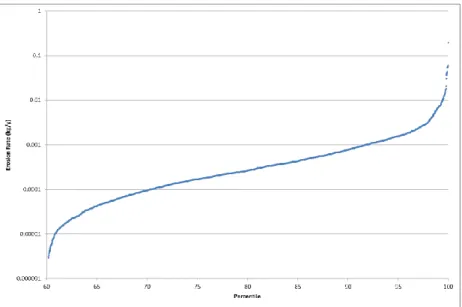
Figure 3 shows the percentage of deposition holes that achieve erosion below a given rate. Approximately 92% of the deposition holes achieve erosion rates of <1 g/y, 99.3% achieve <10 g/y, and only one deposition hole experiences >100 g/y.

(20)

Figure 2: Erosion rates (kg/y) obtained in independent calculations. (Results are

identical to those provided in the spreadsheet.) The maximum erosion rate is 0.194 kg/y for deposition hole 2043.

Figure 3: Erosion rates (kg/y) obtained in independent calculations, plotted as percentile

of deposition holes that achieve erosion below a given rate.

2.4 Alternative Transmissivity Models–

Background

The base case DFN assumes that transmissivity is related to the fracture aperture as

𝛿𝑏𝑎𝑠𝑒 = 0.5𝑇0.5. (2-5)

(21)

𝛿𝑎𝑙𝑡= 0.28𝑇0.3. (2-6)

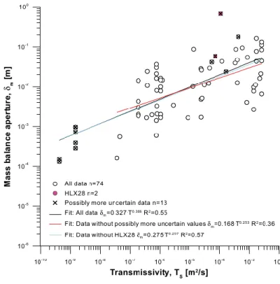
This relationship was derived from a compilation of tracer test data from multiple sites in Sweden (Studsvik, Stripa, Finnsjön, Äspö, Forsmark and Laxemar). The fit of the model to the flow path measurement dataset is shown in Figure 4. The relationship 𝛿 = 0.275𝑇0.297_{(which is close to 2-6}

and has an 𝑅2_{error of 0.57) was obtained by excluding two data points}

(referred to as HLX28). This data was felt to be more uncertain since the pump tests at Laxemar from which it was obtained were performed by pumping in a different feature from the one in which the tracer injection took place. A similar fit to another subset of the data (R-09-28, Figure 6-10) obtains 𝛿 = 0.281𝑇0.295_{, with an 𝑅}2_{error of 0.44 and in another fit (R-09-28,}

Figure 6-16) where only the subset of fractures where apparent storativity is available 𝛿 = 0.282𝑇0.310_{is obtained, with an 𝑅}2_{error of 0.35. When the}

full dataset was used, the best fit was found to be 𝛿 = 0.33𝑇0.31_.

Figure 4: Model fit of mass balance aperture vs. transmissivity for flow path

measurements from multiple sites, using the relationship 𝜹 = 𝜶𝑻𝜷_{(from R-09-28, Figure}

6-5).

The fit derived in R-09-28 is for the ‘mass balance aperture’, which is defined to be the aperture measure that, when combined with appropriate geometrical assumptions leads to a volume that is equal to the mean residence time in the fracture multiplied by the flow rate. R-09-28 explains that of the various measures of aperture that are available, the mass balance aperture has ‘rather good support in the data’ compared to the alternative aperture measures. The aperture-transmissivity model (2-6) will be referred to in this report as the ‘Hjerne model’. TR-10-66, p25 states that (2-6) is

(22)

‘dismissed as being unrealistic for the quantification of buffer erosion (TR-10-52)’,

however TR-10-52, p335 states that

‘the derived mass balance aperture relationship presented by (SKB-R-09-28) should yield apertures on the larger side and is therefore considered appropriate for use as a bounding variant in SR-Site in particle tracking calculations.’.

The argument for the model (2-6) being an upper bound is presented in R-09-22, where it is suggested that since tracer tests are typically performed in fractures that are known to have preferential properties for tracer transport, and also that site-specific electrical resistivity measurements tend to give smaller apertures. However R-09-22 states that electrical resistivity measurements tend to give larger apertures than the SR-Site model (2-5), so by the same argument it could equally be assumed that the SR-Site model is towards a lower bound.

In both (2-5, 2-6), the constants are such that when the aperture is measured in m, the transmissivity is measured in m2/s. It is noted that for a given

transmissivity,

𝛿𝑎𝑙𝑡≅ 0.42 𝛿𝑏𝑎𝑠𝑒0.6 , (2-7)

i.e. that 𝛿𝑎𝑙𝑡> 𝛿𝑏𝑎𝑠𝑒 for apertures of interest (𝛿𝑎𝑙𝑡> 𝛿𝑏𝑎𝑠𝑒 when 𝛿𝑏𝑎𝑠𝑒 <

0.117 m) and so the apertures predicted by 2-6 will be larger than the corresponding ones from the SR-Site model. This would tend to give rise to slower calculated groundwater velocities in the fracture, given the same Darcy velocity, but increases the area of the buffer exposed to erosion.

2.5 Alternative Transmissivity Models - Erosion

Results, Base Case

SKB’s semi-correlated base case DFN results are provided (in the worksheet ‘fs_Q1_2000_pline_merged.ptb’). Whether the provided calculation results can be used to infer the impact upon erosion predictions using the alternative model depends upon how the porosity and/or transmissivity inputs are used in the DFN:

•

If the base case DFN is conditioned on measured or calculated transmissivity data, then (2-6) can be used together with the DFN calculated Darcy flux to infer corresponding fracture apertures and groundwater velocities in the fracture based on the Hjerne model (2-6).

•

If the base case DFN is conditioned on measured or calculated fracture aperture data, then (2-6) should be used to compute alternative transmissivity inputs to the DFN model, which should then be rerun to calculated corresponding Darcy fluxes.

(23)

measured), and that the equivalent hydraulic conductivity of the ECPM block is determined by calculating the response of the ‘mini-DFN’ in each ECPM block to linear head gradients in each of the coordinate axis directions to form an anisotropic hydraulic conductivity tensor.

Therefore, it is possible to estimate the effect of the alternative porosity-transmissivity model (2-6) on the rate of erosion by using (2-1), with the fracture aperture 𝛿 = 𝛿𝑎𝑙𝑡 inferred from the DFN output ‘TRAPP’ according

to (2-6), and the velocity 𝑣 calculated from the Darcy velocity output ‘U0’ of the DFN as described in Section 2.2, but again with 𝛿 = 𝛿𝑎𝑙𝑡. To be clear, the

steps to follow to calculate the erosion rate under the alterative porosity-transmissivity assumption are:

•

Calculate T from the TRAPP (δbase) output of the DFN using (2-5)

•

Calculate δalt using (2-6)

•

Calculate the groundwater velocity valt from the U0 output of the

DFN using (2-3) or (2-4) with δ = δalt

•

Calculate the erosion rate Rerosion,alt using (2-1) with v = valt and

δ = δalt

(Equation (2-7) could be used in place of the first two steps.)

Erosion rates based on the Hjerne model (2-6) are provided by SKB in the ‘velocities_hjerne’ worksheet. The erosion rates based on (2-6) that were independently calculated are different to those supplied. It appears that the difference is caused due to the third step above being missed so that 𝑣 = 𝑣𝑏𝑎𝑠𝑒

is used in the final step. This would appear to be an error and results in a faster groundwater flow rate being used in SKB’s erosion calculation, which therefore increases the calculated rate of erosion.

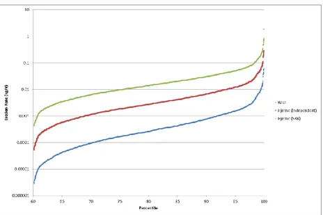
The calculated erosion rates are shown in Figure 5 as percentiles of deposition holes achieving erosion below specified rates. Also plotted are the rates of erosion when the base porosity-transmissivity assumption (2-5) is used and the seemingly erroneous rates calculated by SKB in the ‘velocities_hjerne’ worksheet, which attempts to use (2-6).

The data is summarised in Table 1. With the alternative relationship (2-6), 15 deposition holes experience erosion greater than 0.1 kg/y (compared to one when (2-5) is used) and 446 (7% of) deposition holes experience erosion greater than 0.01 kg/y (compared to 36 when (2-5) is used).

(24)

Figure 5: Erosion rates (kg/y) for the different porosity-transmissivity models: blue -base

(𝜹 = 𝟎. 𝟓𝑻𝟎.𝟓_{); red - alternative (𝜹 = 𝟎. 𝟐𝟖𝑻}𝟎.𝟑_{), obtained in independent calculations;}

green - alternative (𝜹 = 𝟎. 𝟐𝟖𝑻𝟎.𝟑_{), obtained by SKB. Erosion rates are plotted as}

percentile of deposition holes that achieve erosion below a given rate.

Table 1: Percentage of deposition holes that achieve erosion below a given rate for the

base (𝜹 = 𝟎. 𝟓𝑻𝟎.𝟓_{) and alternative (𝜹 = 𝟎. 𝟐𝟖𝑻}𝟎.𝟑_{) porosity-transmissivity models.}

Percentage of deposition holes that achieve erosion below given rate

Base model 𝛅𝐛𝐚𝐬𝐞= 𝟎. 𝟓𝐓𝟎.𝟓

Alternative (Hjerne) model 𝛅𝐚𝐥𝐭= 𝟎. 𝟐𝟖𝐓𝟎.𝟑

< 𝟏𝒆−𝟓_kg/y ₆₁ _-

< 𝟏𝒆−𝟒_kg/y ₇₀ ₆₀

< 𝟏𝒆−𝟑_kg/y ₉₂ ₆₉

< 𝟏𝒆−𝟐_kg/y _99.3 ₉₃

< 𝟏𝒆−𝟏_kg/y _{99.9 (all but one)} _{99.8 (15 above 0.1 kg/y)}

2.6 Establishment of Advective Conditions in

the Deposition Hole – Base Case

The erosion rates calculated in Sections 2.3 and 2.5 can be used to determine the number of deposition holes that experience advective conditions (for the first time) during each glacial cycle by determining the time taken to erode a volume sufficient for advection to take place. TR-10-66 suggests the approximation

𝑉𝑧𝑜𝑛𝑒 =ℎ𝑧𝑜𝑛𝑒𝜋(𝑟ℎ

2_−𝑟 𝑐𝑎𝑛2 )

2

to determine the volume of the eroded zone, 𝑉𝑧𝑜𝑛𝑒. The approximation

(25)

ℎ𝑧𝑜𝑛𝑒= 𝑑𝑏𝑢𝑓 (the buffer thickness), which assumes that the thickness of the

eroded area is the same in the horizontal and vertical directions. The mass of buffer that must be eroded before advective conditions occur adjacent to the canister surface is then 𝑀𝑎𝑑𝑣 = 𝑉𝑧𝑜𝑛𝑒𝜌𝑏𝑢𝑓, where 𝜌𝑏𝑢𝑓 (kg/m3) is the saturated

buffer density. The values of the relevant input parameters are given in Table 2 and result in an eroded volume 𝑉𝑧𝑜𝑛𝑒 = 0.27 m3 and an eroded mass

𝑀𝑎𝑑𝑣= 531 kg. This derivation assumes that no re-homogenisation of the

buffer takes place to close the eroded gap, and therefore 531 kg can be taken to be a pessimistic value. In TR-10-66, SKB assume a base case mass of eroded buffer to be 1,200 kg and vary the amount between 600 kg and 2,400 kg in their sensitivity analysis, but the reasoning for these values (or a corresponding reference) is not presented in TR-10-66. The value appears to derive from discussion in TR-11-01 (p387) in which modelling is referred to that demonstrated that even when two entire bentonite rings (with a dry mass of 2,400 kg) are omitted from the buffer, the buffer is able to re-homogenise and almost maintain the minimum dry density in the buffer (1,000 kg/m3). The value of 1,200 kg therefore corresponds to a ‘half annulus’.

Table 2: Properties used in erosion time calculations.

Property Value Source / Notes 𝒓𝒄𝒂𝒏 0.525 m TR-10-66, p11

𝒅𝒃𝒖𝒇 0.35 m TR-10-66, p22 (and the assumption

𝒉𝒛𝒐𝒏𝒆= 𝒅𝒃𝒖𝒇 is made, consistent with

TR-10-66)

𝒓𝒉 0.875 m (Inferred from 𝒓𝒄𝒂𝒏 and 𝒅𝒃𝒖𝒇)

𝝆𝒃𝒖𝒇 1971 kg/m3 Assumes dry density of 1571 kg/m3 (TR-10-66, p31) and a porosity of 0.4 (TR-10-66, p27).

Deposition holes that would be excluded on the basis of the 𝐹𝑃𝐶 (𝐹𝑃𝐶 < 1) or the 𝐸𝐹𝑃𝐶 (𝐸𝐹𝑃𝐶 < 5) are excluded from the erosion timescale

calculations, consistent with the calculations presented in TR-10-66, Section 5.3.5 (but in contrast to the analysis in Section 2.2-2.3, in which depositions with 𝐹𝑃𝐶 = 1 were included in the analysis).

The number of deposition holes experiencing advective conditions adjacent to the canister (for the first time) during each glaciation is shown in Table 3 for the base and alternative porosity-transmissivity relationships. Also shown are the same results when the eroded mass required for advection, 𝑀𝑎𝑑𝑣, is set to

1,200 kg (the ‘base case’ value – TR-10-66, p40).

The same results are also shown in Figure 6 (𝑀𝑎𝑑𝑣= 1,200 kg) and Figure 7

(𝑀𝑎𝑑𝑣= 531 kg). The calculations assume a glacial period of length 120,000

y, with dilute water assumed to be flowing at repository depths for 25% of the glacial cycle period, consistent with the assumptions made in TR-10-66 (p37). It is clear that a significantly greater number of deposition holes experience advective conditions when the alternative porosity-transmissivity model (2-6) is used. For example, during the first five glacial periods 294 locations experience advective conditions when the Hjerne model is assumed,

(26)

advective in each glacial period is different (Figure 7). In this case there is a big increase in the early glacial cycles, with the number of new deposition holes becoming advective falling off thereafter. Effectively, since the required eroded mass is more than halved, deposition holes that would have required one or two glacial periods, and some that would have required three glaciations, become advective during the first glacial period, and so on.

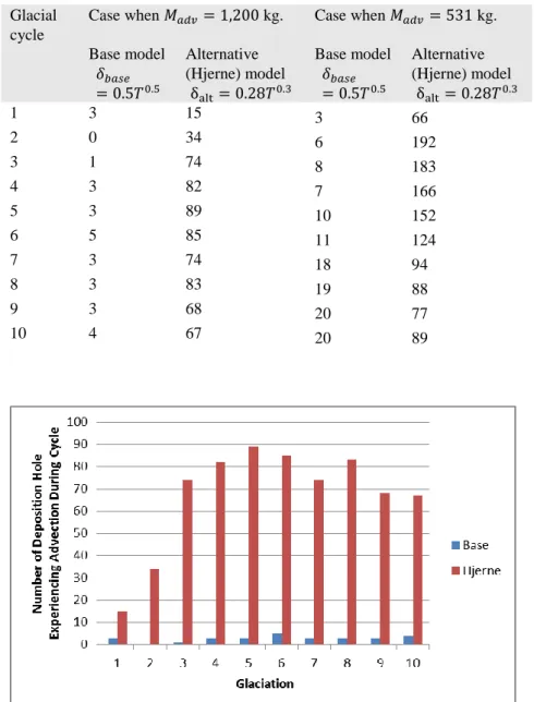
Table 3: Number of deposition holes experiencing advective conditions for the first time

during each glacial cycle for the base and alternative (Hjerne) porosity-transmissivity models assuming 𝑴𝒂𝒅𝒗= 𝟏, 𝟐𝟎𝟎 kg and 𝑴𝒂𝒅𝒗= 𝟓𝟑𝟏 kg.

Glacial cycle

Case when 𝑀𝑎𝑑𝑣= 1,200 kg. Case when 𝑀𝑎𝑑𝑣= 531 kg.

Base model 𝛿𝑏𝑎𝑠𝑒 = 0.5𝑇0.5 Alternative (Hjerne) model δalt= 0.28𝑇0.3 Base model 𝛿𝑏𝑎𝑠𝑒 = 0.5𝑇0.5 Alternative (Hjerne) model δalt= 0.28𝑇0.3 1 3 15 ₃ ₆₆ 2 0 34 ₆ ₁₉₂ 3 1 74 ₈ ₁₈₃ 4 3 82 ₇ ₁₆₆ 5 3 89 ₁₀ ₁₅₂ 6 5 85 ₁₁ ₁₂₄ 7 3 74 ₁₈ ₉₄ 8 3 83 ₁₉ ₈₈ 9 3 68 ₂₀ ₇₇ 10 4 67 ₂₀ ₈₉

Figure 6: Number of deposition holes experiencing advective conditions for the first time

during each glacial cycle for the base and alternative (Hjerne) porosity-transmissivity models assuming 𝑴𝒂𝒅𝒗= 𝟏, 𝟐𝟎𝟎 kg (see Table 3).

(27)

Figure 7: Number of deposition holes experiencing advective conditions for the first time

during each glacial cycle for the base and alternative (Hjerne) porosity-transmissivity models assuming 𝑴𝒂𝒅𝒗= 𝟓𝟑𝟏 kg (see Table 3).

2.7 Establishment of Advective Conditions in

the Deposition Hole – Other SKB DFN

Realisations

The analysis presented in Section 2.6 determined the time required for erosion to establish advective conditions in the deposition holes in the base case DFN model. A selection of other DFN cases has also been provided, and is described in Appendix A. In all, there are 25 sets of results in total. The cases comprise:

•

(#2) Ten alternative realisations of the base case;

•

(#3) Four realisations of the correlated size-transmissivity case;

•

(#4) Four realisations of the truncated, uncorrelated size-transmissivity case;

•

(#5) Two realisations with different EDZ transmissivities;

•

(#6) A variant with no EDZ;

•

(#7) Three realisations with possible deformation zones included; and

•

(#8) A tunnel variant with crown space.

(Model numbers #n in parenthesis correspond to the axis labels in Figure 8 and Figure 9, which will be discussed later. The base case DFN model is referred to as #1.)

Two additional cases were also provided in the file

merged/100610_fs_top25_Q123_2000_pline10_merged_ptb.zip, which correspond to ‘Multiple particles per start point from 25% highest U0 locations in hydro base case at 2000 AD’. The precise background to these

(28)

Since there are several sets of results, the analysis is performed using a script (described in Appendix C) rather than implementing the calculations in several spreadsheets.

The number of deposition holes experiencing advective conditions for the first time during the first five glacial cycles for each of the above cases is shown in Table 4 for both the base and Hjerne aperture-transmissivity relationships. The corresponding results for the base case (from Table 3) are also shown. The correlated and uncorrelated size-transmissivity cases and the base case (in which a semi-correlated model is assumed) lead to similar numbers of advective deposition holes after the first glaciation (2, 1.5 and 1.7 respectively) for the base aperture-transmissivity model. However the uncorrelated model leads to significantly more advective deposition holes in subsequent glaciations (averaging 15.75, 29.5, 39.5 and 43.5 respectively for the second, third fourth and fifth glaciations) compared to the correlated model (8.25, 9.25, 8.5 and 6.25 respectively) and base case (1.2, 0.9, 1.8 and 2 respectively).

The use of the Hjerne aperture-transmissivity model leads to significantly more advective deposition holes, especially in the uncorrelated and correlated models, with an average of 46.75, 86.25, 118.25, 113.5 and 118.25 over the first five glaciations in the case of the correlated size-transmissivity relationship and 158.5, 343.5, 289.5, 232.25 and 117.5 in the uncorrelated size-transmissivity case.

The other cases that were considered (the EDZ variants and the tunnel with crown space model) each lead to similar numbers of advective deposition holes as the base case.

Over the first 8 glacial periods (corresponding to a total evolution of 960,000 y) the average of the total number of advective positions for the Hjerne realisations of the base case is 537 holes. This number agrees quite well with the 575 positions quoted by SKB for the pessimistic fracture aperture case in Figure 12-3 of TR-11-01.

The analogous results when the amount of buffer required to be eroded before advection can begin is assumed to be 531 kg are shown in Table 5. In this case the correlated and uncorrelated size-transmissivity cases lead to more advective deposition holes in all glacial periods (not just the second period onwards, as was the case when the eroded mass was 1,200 kg). The correlated model gives 13.5, 18, 19.3, 21, 23,25 and the uncorrelated model gives 23.8, 87.25, 105, 106, 105 newly advective deposition holes in the first five glacial periods, compared to the base case giving 3, 3.6, 6.6, 8.2, 12.4. Again, the other cases that were considered (the EDZ variants and the tunnel with crown space model) each lead to similar numbers of advective deposition holes as the base case.

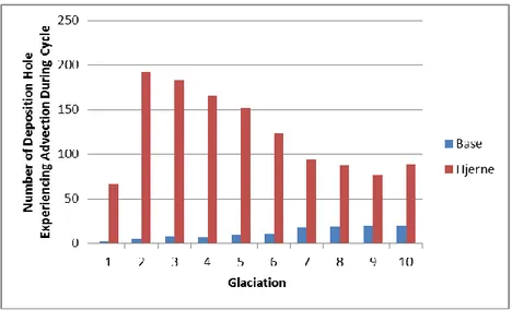
The results for the 1,200 and 531 kg eroded masses are shown graphically in the bar charts in Figure 8 and Figure 9 respectively, which show the number of deposition holes becoming advective in each of the first five glacial periods for each of the models, assuming both the base and Hjerne

(29)

aperture-The results for the DFN model corresponding to the 25% highest U0 locations in the hydrogeological base case are shown in Table 5 for both the 1,200 and 531 kg of eroded buffer cases. These cases result in far greater numbers of deposition holes becoming advective in the first glacial period (~2,000 deposition holes for both the base and Hjerne models). It would therefore appear that these cases represent a different form of output that is maybe not compatible with this analysis.

Appendix E presents an independent attempt to reproduce results of numbers of eroded locations in SKB’s probabilistic analysis that are presented in TR-11-01 Figure 12-4.

(30)

Table 4: Number of deposition holes experiencing advective conditions for the first time during each glacial cycle for the base and alternative (Hjerne) porosity-transmissivity models

assuming 𝑴𝒂𝒅𝒗= 𝟏, 𝟐𝟎𝟎 kg.

Base Aperture-Transmissivity Hjerne Aperture-Transmissivity Glaciation number Glaciation number

1 2 3 4 5 1 2 3 4 5 #1 Base case

fs_Q1_2000_pline_merged.xls 3 0 1 3 3 15 34 74 82 90 #2 Ten alternative realisations of the base case

fs_r1_Q1_2000_pline_merged.xls 2 1 1 3 4 16 38 63 95 84 fs_r3_Q1_2000_pline_merged.xls 2 3 0 0 1 9 50 76 74 83 fs_r4_Q1_2000_pline_merged.xls 0 0 0 1 1 11 36 88 105 93 fs_r5_Q1_2000_pline_merged.xls 0 1 0 1 2 6 55 70 72 94 fs_r6_Q1_2000_pline_merged.xls 0 1 0 1 1 8 41 75 91 89 fs_r7_Q1_2000_pline_merged.xls 2 3 5 2 5 23 37 76 86 72 fs_r8_Q1_2000_pline_merged.xls 1 1 1 1 0 4 23 53 90 73 fs_r9_Q1_2000_pline_merged.xls 5 1 0 3 2 19 35 62 92 73 fs_r10_Q1_2000_pline_merged.xls 0 0 1 3 2 6 41 82 77 88 fs_r12_Q1_2000_pline_merged.xls 5 1 1 3 2 15 32 67 88 79 Average 1.7 1.2 0.9 1.8 2 11.7 38.8 71.2 87 82.8 #3 Four realisations of the correlated size-transmissivity case

(31)

1 2 3 4 5 1 2 3 4 5 fs_r2_corr_Q1_2000_pline_merged.xls 2 4 3 3 6 29 101 118 116 124 fs_r4_corr_Q1_2000_pline_merged.xls 0 14 26 10 7 73 86 134 135 130 fs_r5_corr_Q1_2000_pline_merged.xls 2 9 6 12 10 51 70 92 95 114 Average 2 8.25 9.25 8.5 6.25 46.75 86.25 118.25 113.5 118.25

(32)

Table 4 (continued)

1 2 3 4 5 1 2 3 4 5 #4 Four realisations of the truncated, uncorrelated size-transmissivity case

fs_uncorr_truncHCD_Q1_2000_pline_merged.xls 1 17 30 47 40 166 327 276 200 172 fs_r2_uncorr_truncHCD_Q1_2000_pline_merged.xls 1 12 23 30 39 134 322 280 236 180 fs_r3_uncorr_truncHCD_Q1_2000_pline_merged.xls 4 19 34 38 48 172 379 278 235 166 fs_r5_uncorr_truncHCD_Q1_2000_pline_merged.xls 0 15 31 43 47 162 346 324 258 192 Average 1.5 15.75 29.5 39.5 43.5 158.5 343.5 289.5 232.25 177.5 #5 Two realisations with different EDZ transmissivity

fs_maxedz_6_Q1_2000_pline_merged.xls 3 1 4 8 4 24 41 87 83 88 fs_maxedz_7_Q1_2000_pline_merged.xls 3 0 1 4 4 17 40 79 89 101 Average 3 0.5 2.5 6 4 20.5 40.5 83 86 94.5 #7 Three realisations with possible deformation zones included

fs_pdzr1_Q1_2000_pline_merged.xls 2 1 1 3 4 16 36 74 96 92 fs_pdzr2_Q1_2000_pline_merged.xls 5 1 2 2 2 16 34 65 93 79 fs_pdzr3_Q1_2000_pline_merged.xls 2 3 0 0 1 9 52 74 87 73 Average 3 1.67 1 1.67 2.33 13.67 40.67 71 92 81.33 #6 No EDZ case fs_noedz_Q1_2000_pline_merged.xls 2 1 1 3 3 14 20 34 45 54 #8 Tunnel variant with crown space

(33)

fs_crown_Q1_2000_pline_merged.xls 3 0 1 4 5 22 37 63 79 95

assuming 𝑴𝒂𝒅𝒗= 𝟓𝟑𝟏 kg.

1 2 3 4 5 1 2 3 4 5 #1 Base case (two identical cases, one with extra TRAPP output)

fs_Q1_2000_pline_merged.xls 3 6 8 7 10 66 192 183 166 152 #2 Ten alternative realisations of the base case

fs_r1_Q1_2000_pline_merged.xls 3 6 9 11 12 67 189 201 163 160 fs_r3_Q1_2000_pline_merged.xls 5 0 3 10 23 84 171 172 168 164 fs_r4_Q1_2000_pline_merged.xls 0 2 11 7 14 68 228 197 163 140 fs_r5_Q1_2000_pline_merged.xls 1 3 5 10 15 83 160 196 180 146 fs_r6_Q1_2000_pline_merged.xls 1 2 8 3 12 70 190 192 179 154 fs_r7_Q1_2000_pline_merged.xls 5 8 13 8 12 79 185 165 168 166 fs_r8_Q1_2000_pline_merged.xls 3 1 0 5 5 38 177 206 146 167 fs_r9_Q1_2000_pline_merged.xls 6 4 7 9 8 68 186 174 168 147 fs_r10_Q1_2000_pline_merged.xls 0 6 5 8 12 67 181 204 190 153 fs_r12_Q1_2000_pline_merged.xls 6 4 5 11 11 60 184 173 148 132

(34)

1 2 3 4 5 1 2 3 4 5 Average 3 3.6 6.6 8.2 12.4 68.4 185.1 188 167.3 152.9 #3 Four realisations of the correlated size-transmissivity case

fs_corr_Q1_2000_pline_merged.xls 11 11 16 24 23 163 249 295 318 269 fs_r2_corr_Q1_2000_pline_merged.xls 8 7 21 24 26 163 259 351 309 289 fs_r4_corr_Q1_2000_pline_merged.xls 20 35 16 23 26 186 313 327 335 238 fs_r5_corr_Q1_2000_pline_merged.xls 15 19 24 13 18 147 221 292 300 254 Average 13.5 18 19.3 21 23.25 164.8 260.5 316.25 315.5 262.5 Table 5 (continued)

1 2 3 4 5 1 2 3 4 5 #4 Four realisations of the truncated, uncorrelated size-transmissivity case

fs_uncorr_truncHCD_Q1_2000_pline_merged.xls 24 99 109 94 99 571 486 317 210 129 fs_r2_uncorr_truncHCD_Q1_2000_pline_merged.xls 19 67 99 102 93 534 538 283 209 110 fs_r3_uncorr_truncHCD_Q1_2000_pline_merged.xls 28 94 107 113 122 630 535 292 197 127 fs_r5_uncorr_truncHCD_Q1_2000_pline_merged.xls 24 89 106 116 106 593 599 296 176 113 Average 23.8 87.25 105 106 105 582 539.5 297 198 119.75

(35)

1 2 3 4 5 1 2 3 4 5 #5 Two realisations with different EDZ transmissivities

fs_maxedz_6_Q1_2000_pline_merged.xls 4 14 7 9 8 83 204 172 169 142 fs_maxedz_7_Q1_2000_pline_merged.xls 4 5 12 7 8 76 195 186 167 140 Average 4 9.5 9.5 8 8 79.5 199.5 179 168 141 #7 Three realisations with possible deformation zones included

fs_pdzr1_Q1_2000_pline_merged.xls 3 6 10 8 12 71 195 200 164 156 fs_pdzr2_Q1_2000_pline_merged.xls 6 4 6 10 14 64 191 172 149 140 fs_pdzr3_Q1_2000_pline_merged.xls 5 0 4 7 25 84 176 171 172 160 Average 4.67 3.33 6.67 8.33 17.00 73.00 187.33 181 161.67 152.00 #6 No EDZ case fs_noedz_Q1_2000_pline_merged.xls 3 6 6 5 8 46 98 104 105 81 #8 Tunnel variant with crown space

(36)

Figure 8: Number of deposition holes experiencing advective conditions for the first time during each glacial cycle for the base and alternative (Hjerne) porosity-transmissivity models

assuming 𝑴𝒂𝒅𝒗= 𝟏, 𝟐𝟎𝟎 kg. Summarises data shown in Table 4 – see the introduction to Section 2.7 for a description of the model numbers (x axis label). The groups of five same

coloured bars shows the number of deposition holes in the first five glacial periods. 0 50 100 150 200 250 300 350 400 1 2 3 4 5 6 7 8 Nu m b er of A d vec ti ve D ep osi ti on H oles in Gl aci al P er iod s 1 -5 Model # Base Hjerne

(37)

Figure 9: Number of deposition holes experiencing advective conditions for the first time during each glacial cycle for the base and alternative (Hjerne) porosity-transmissivity models

assuming 𝑴𝒂𝒅𝒗= 𝟓𝟑𝟏 kg. Summarises data shown in Table 5 – see the introduction to Section 2.7 for a description of the model numbers (x axis label). The groups of five same

coloured bars shows the number of deposition holes in the first five glacial periods. 0 100 200 300 400 500 600 700 1 2 3 4 5 6 7 8 N u m b e r o f A d ve ctiv e D e p o si tion H o le s in G lac ial Per io d s 1 -5 Model # Base Hjerne

(38)

assuming 𝑴𝒂𝒅𝒗= 𝟏, 𝟐𝟎𝟎 and 𝑴𝒂𝒅𝒗= 𝟓𝟎𝟎 kg in the DFN case corresponding to the 25% highest U0 locations in hydrogeological base case.

1 2 3 4 5 1 2 3 4 5 𝑀𝑎𝑑𝑣= 1,200 kg fs_top25_Q1_2000_pline10_merged.xls 30 0 10 70 60 230 420 990 1180 1140 fs_top25_Q1_2000_pline_merged.xls 3 0 1 3 3 15 34 74 82 90 𝑀𝑎𝑑𝑣 = 531 kg fs_top25_Q1_2000_pline10_merged.xls 30 130 110 80 130 890 2590 2150 1840 1680 fs_top25_Q1_2000_pline_merged.xls 3 6 8 7 10 66 192 183 166 152

(39)

2.8 Summary of Corrosion Model for Advective

Conditions in TR-10-66

SKB’s corrosion model for advective conditions is summarised in TR-10-66, Section 4.3.2. The rate of corrosion depends upon the equivalent flow rate of corrodants to the canister surface, 𝑄𝑒𝑞 (m3/y) which is given by TR-10-66, eq

(4-22/23), 𝑄𝑒𝑞= { 𝑞𝑒𝑏 𝑞𝑒𝑏≤ 𝑞lim, 1.13√𝑞𝑒𝑏𝐷𝑤𝑉𝑧𝑜𝑛𝑒 𝑑_𝑏𝑢𝑓 𝑞𝑒𝑏> 𝑞lim. (2-8)

Here, 𝑞𝑒𝑏 (m3/y) is the “water flux through the part of the fracture that intersects the

deposition hole”, 𝐷𝑤 (m2/s) is the diffusion coefficient of the corrodant solute in

water, 𝑉𝑧𝑜𝑛𝑒 (m3) is the volume of buffer that has been eroded, 𝑑𝑏𝑢𝑓 (m) is the buffer

thickness and the constant 1.13 is more accurately given by 2/√𝜋. The flux 𝑞lim

defines a “high flow rate”.

No value for 𝑞lim is given in TR-10-66, but the appendix of TR-10-42 provides a

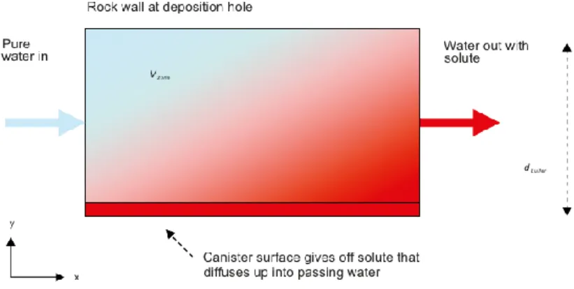
derivation based on an analytical solution to an advection-diffusion problem. The geometry assumed in the analysis is shown in Figure 10.

In the setting of Figure 10, 𝑞lim is determined to be the limiting (slow) flow rate into

the deposition hole at which the solute is able to diffuse across the eroded buffer to establish a mean concentration of solute in the eroded buffer, 𝑐𝑚𝑒𝑎𝑛, that is equal to

the concentration of the solute at the bottom boundary, 𝑐0 (i.e. the concentration is

uniform and equal to 𝑐0 across the eroded buffer). 𝑄𝑒𝑞 is related to 𝑞𝑒𝑏 by

𝑄𝑒𝑞𝑐0= 𝑞𝑒𝑏𝑐𝑚𝑒𝑎𝑛 (2-9)

and, for small residence times 𝑡𝑟𝑒𝑠 (y) in the buffer (i.e. for fast flow rates), 𝑐𝑚𝑒𝑎𝑛

and 𝑐0 are related approximately as (Bird et al., 2002) 𝑐_{𝑚𝑒𝑎𝑛} 𝑐0 = 2 √𝜋 √𝐷𝑤𝑡𝑟𝑒𝑠 𝑑_{𝑏𝑢𝑓𝑓𝑒𝑟}. (2-10)

The approximation becomes invalid for residence times above a sufficiently long residence time 𝑡lim, since the physical constraint 𝑐𝑚𝑒𝑎𝑛≤ 𝑐0 must always be

(40)

Figure 10: Geometry assumed in the analysis presented in the appendix of TR-10-42

(reproduced from TR-10-42, Fig A1).

[The approximation 𝑡𝑟𝑒𝑠 = 𝑉𝑧𝑜𝑛𝑒/𝑞𝑒𝑏 is made in the analysis, which assumes that

the inflowing water is ‘perfectly mixed’ around the eroded buffer. This is a valid assumption within the simplified 2-D geometry of Figure 10, but when the aperture of the intersecting fracture is much smaller than the height of the eroded buffer section, ℎ𝑧𝑜𝑛𝑒 (Section 2.6), it would seem possible that 𝑡𝑟𝑒𝑠< 𝑉𝑧𝑜𝑛𝑒/𝑞𝑒𝑏 on average

for the solute particles, so it is not clear that the approximation is a good one in the 3-D eroded geometry.]

Using the approximation 𝑡𝑟𝑒𝑠= 𝑉𝑧𝑜𝑛𝑒/𝑞𝑒𝑏, a limiting water flux corresponding to

𝑡lim can be denoted 𝑞lim, for which the approximation (2-10) becomes invalid when

𝑞𝑒𝑏< 𝑞lim. The value of 𝑞lim can be found, by setting 𝑐𝑚𝑒𝑎𝑛= 𝑐0 in (2-10),

𝑞lim= 4 𝜋

𝐷_𝑤𝑉_{𝑧𝑜𝑛𝑒}

𝑑_{𝑏𝑢𝑓𝑓𝑒𝑟}2 . (2-11)

Rearranging (2-9) and (2-10) allows the case 𝑞𝑒𝑏> 𝑞lim in (2-8) to be obtained. The

limit 𝑐𝑚𝑒𝑎𝑛= 𝑐0 is equivalent to the condition 𝑄𝑒𝑞= 𝑞𝑒𝑏 (from (2-9)) and therefore

the flux limit 𝑞lim can also be considered to be the flux at which 𝑄𝑒𝑞 and 𝑞𝑒𝑏 become

equal. For flows with 𝑞𝑒𝑏≤ 𝑞lim, it will be the case that 𝑐𝑚𝑒𝑎𝑛= 𝑐0, and therefore

in this flow regime 𝑄𝑒𝑞 = 𝑞𝑒𝑏 by (2-9).

It is noted that in the context of a corroding solute travelling to the canister surface it is assumed that 𝑐0= 0 (i.e. all sulphide is consumed in corrosion reactions at the

canister surface), and therefore the analysis of TR-10-42 would seem to break down since it suggests that there is a limiting flux 𝑞lim (which is greater than zero by

(2-11)) at which the mean sulphide concentration across the eroded buffer would be zero, but this can never be the case for a solute that is arriving from the inflowing boundary of Figure 10. Therefore it would seem that the part of this analysis related to 𝑞lim is not necessarily applicable to the corrosion case (and is only relevant for

models of solute release form the canister surface). In this case, a conservative assumption would be to assume that 𝑄𝑒𝑞= 𝑞𝑒𝑏 always, i.e. that the equivalent flux

is directly equal to the water flux, meaning that all incoming solute is consumed in the corrosion reaction.

(41)

𝑞𝑒𝑏= 𝑓𝑐𝑜𝑛𝑐2𝑟ℎℎ𝑐𝑎𝑛𝑈0. (2-12)

Here 𝑓𝑐𝑜𝑛𝑐 is a flow concentration factor accounting for the focussing of flows into

the eroded void. The area scaling 2𝑟ℎℎ𝑐𝑎𝑛 was explained in Section 2.2. Given 𝑞𝑒𝑏,

𝑄𝑒𝑞 can be calculated by (2-8) and then the rate of corrosion 𝑣𝑐𝑜𝑟𝑟 (m/y) caused by

the mass transport of corrodant is given by TR-10-66, equation (4-25) 𝑣𝑐𝑜𝑟𝑟= 𝑄𝑒𝑞[HS−]𝑓𝐻𝑆_𝜌𝑀𝐶𝑢

𝐶𝑢

1

𝐴𝑐𝑜𝑟𝑟 (2-13)

where [HS−_{] (mol/m}3_{) is the concentration of sulphide in the groundwater, 𝑓}

𝐻𝑆= 2

is a stoichiometric factor relating the number of moles of copper consumed in the corrosion reaction per mole of sulphide, 𝑀𝐶𝑢 (kg/mol) and 𝜌𝐶𝑢 (kg/m3) are the molar

weight and density of copper respectively, and 𝐴𝑐𝑜𝑟𝑟 (m2) is the area over which

corrosion is assumed to occur (i.e. the copper surface area exposed by corrosion). The only terms in the analysis so far unaccounted for are the geometric factors 𝑉𝑧𝑜𝑛𝑒

and 𝐴𝑐𝑜𝑟𝑟, which both depend on the assumptions made regarding the geometry of

the eroded volume.

In the absence of a detailed model for the development of the eroded void volume, SKB assume that the by the time that the surface of the canister is exposed, the void has a rectangular cross-section and that only the upstream half of the buffer is eroded. Therefore when the eroded volume reaches the canister surface,

𝑉𝑧𝑜𝑛𝑒 =ℎ𝑧𝑜𝑛𝑒 𝜋(𝑟ℎ

2_−𝑟 𝑐𝑎𝑛2 )

2 , (2-14)

where ℎ𝑧𝑜𝑛𝑒 (m) is the height of the eroded void. SKB assume that the eroded depth

is equal to this height, so that ℎ𝑧𝑜𝑛𝑒= 𝑑𝑏𝑢𝑓, and acknowledge that this assumption

is ‘a bit crude’.

In SKB (2011), SKB note that equation (2-14) was implemented erroneously in the calculations performed in TR-10-66 and that the trailing divide by 2 was omitted from the calculation, so that

𝑉𝑧𝑜𝑛𝑒 = ℎ𝑧𝑜𝑛𝑒 𝜋(𝑟ℎ2− 𝑟𝑐𝑎𝑛2 )

was used. The consequence of the error is that that value of 𝑞lim is twice as large as

intended, by (2-11), which affects the ‘switch’ in equation (2-8) that is used to determine 𝑄𝑒𝑞. This results in more locations satisfying 𝑞𝑒𝑏≤ 𝑞lim (in which case

𝑄𝑒𝑞= 𝑞𝑒𝑏 is assumed) and for those locations for which it is still true that 𝑞𝑒𝑏>

𝑞lim, the resulting value of 𝑄𝑒𝑞 is a factor of √2 too large.

In both cases a value of 𝑄𝑒𝑞 is obtained that is larger than if (2-14) had been

implemented correctly, and by (2-13) this results in a larger corrosion rate than intended. The mistake therefore leads to a pessimistic estimate of the corrosion rate compared to the intended calculation.

From (2-13) it is clear that a larger exposed area will lead to smaller depths of corrosion. Following the assumed rectangular eroded volume, SKB assume that the height of the exposed area ℎ𝑐𝑜𝑟𝑟 (m) is equal to ℎ𝑧𝑜𝑛𝑒 (= 𝑑𝑏𝑢𝑓). Given ℎ𝑧𝑜𝑛𝑒, 𝐴𝑐𝑜𝑟𝑟

(42)

𝐴𝑐𝑜𝑟𝑟 = 𝜋𝑟𝑐𝑎𝑛ℎ𝑐𝑜𝑟𝑟 (2-15)

(since only the upstream half of the deposition hole is assumed to be eroded). SKB also present a more conservative approach to determine ℎ𝑐𝑜𝑟𝑟 (m), in which it

is assumed that prior to the rectangular void cross section (discussed above) develops by growing the void as a semi-circular cross section, until the copper surface is reached. Then erosion is assumed to halt as soon as a band of the canister surface is exposed whose height ℎ𝑐𝑜𝑟𝑟 (m) is given by

ℎ𝑐𝑜𝑟𝑟=𝜋𝑑₂𝐶𝑢 (2-16)

where 𝑑𝐶𝑢 (m) is the copper thickness. The height is obtained by equating a

hypothetical rectangular cross-sectional corrosion area ℎ𝑐𝑜𝑟𝑟𝑑𝐶𝑢 to a hypothetical

semi-circular cross-sectional corrosion area 𝜋𝑑𝐶𝑢2 /2. The semi-circular corrosion

cross-section in the copper that is assumed is almost certainly not realistic (it would imply that rates of corrosion are somehow proportional to the rate at which the canister surface area is exposed by erosion), but is nevertheless clearly a

conservative assumption, since it is unlikely that erosion would halt after exposing such a small fraction of the surface area in precisely the way that is assumed. Results presented in Figure 5-9 of TR-10-66 suggest that the assumption of this more pessimistic corrosion geometry increases the mean number of failed canisters in 106 year by a factor of ~5 (to 0.557) compared to the semi-correlated base case.