2004:05 (SSI 2004:01) Further AMBER and Ecolego Intercomparisons

(1)

SKI Report 2004:05

SSI Report 2004:01

Research

Further AMBER and Ecolego

Intercomparisons

Philip Maul

Peter Robinson

Robert Broed

Rodolfo Avila

January 2004

(2)

(3)

SKI/SSI perspective

Background

As part of preparations for review of future license applications, the Swedish Nuclear Power Inspectorate (SKI) and Swedish Radiation Protection Authority (SSI) are developing their capabilities of doing radionuclide transport calculations. For this purpose SKI and SSI have developed the software program AMBER and Ecolego respectively.

The AMBER compartmental modelling software has been used by Quintessa in undertaking Performance Assessment (PA) calculations for SKI for the last four years. In particular, it was used in helping to identify key issues in the safety case for SFR 1. SSI and the Norwegian Radiation Protection Authority (NRPA) are supporting the development of Ecolego which is based on the Matlab/Simulink general purpose modelling software and provides a user-friendly Graphical User Interface (GUI) which is particularly suitable for undertaking PA calculations.

Purpose of the project

Based on calculation cases considered in SKB’s SR 97, intercomparison calculations using AMBER and Ecolego was done in a previous project (SKI, SSI, 2003). The reasons for undertaking such intercomparisons were to give confidence in the use of AMBER and Ecolego for whole system PA calculations for a deep repository. And to provide SKI and SSI with an understanding of some of the technical issues raised by seeking to repeat the SR 97 calculations with different models and software.

In order to gain more information on the comparisons between the two codes, additional intercomparisons have been undertaken using input data from the Vault Safety Case originally undertaken as part of an IAEA research project (ISAM).

Results

The comparisons between the AMBER and Ecolego calculations for the ISAM vault safety case have shown excellent agreement. Calculations at specified times generally agree to around three significant figures, and calculations of peak radionuclide fluxes and concentrations agree to two significant figures. This agreement is particularly good given the large number of model compartments and the inclusion of decay changes of up to six members.

Project information

SKI project manager: Benny Sundström.

(4)

SKI, SSI, AMBER and Ecolego Intercomparisons using Calculations from SR97, SKI Report 2003:28, SSI report 2003:11, Statens kärnkraftinspektion, Statens strålskydds-institut, Stockholm, 2003.

(5)

SKI Report 2004:05

SSI Report 2004:01

Research

Further AMBER and Ecolego

Intercomparisons

Philip Maul¹ Peter Robinson¹ Robert Broed² Rodolfo Avila³ ¹Quintessa Limited Dalton House Newtown Road Henley-on-Thames Oxfordshire RG9 1HG United Kingdom ²Department of Physics

Center of Physics, Astronomy and Biotechnology AlbaNova University Center

Stockholm University SE-106 91 Stockholm Sweden

(6)

(7)

Summary

The AMBER compartmental modelling software is used by Quintessa in undertaking Performance Assessment (PA) calculations for SKI. SSI and NRPA are supporting the development of Ecolego which is based on the Matlab/Simulink general purpose modelling software for undertaking PA calculations.

Intercomparison calculations using AMBER and Ecolego have been undertaken based on calculation cases considered in SKB's SR97 assessment. The reasons for undertaking such intercomparisons included:

1. to give confidence in the use of AMBER and Ecolego for whole system PA calculations for a deep repository; and

2. to provide SKI and SSI with an understanding of some of the technical issues raised by seeking to repeat the SR97 calculations with different models and software. Conclusions drawn from these intercomparisons included:

1. Both modelling packages successfully reproduced SKB’s SR97 calculations for the near field, geosphere and biosphere.

2. AMBER and Ecolego calculations were typically in agreement to within one significant figure, but in several instances the SR97 documentation was not sufficiently clear to enable the implementation of the models in AMBER and Ecolego to be unambiguous.

In order to gain more information on the comparisons between the two codes, additional intecomparisons have been undertaken using input data from the Vault Safety Case originally undertaken as part of an IAEA research project (ISAM).

The most important situation where agreement may not be as good as that generally found is where radionuclides have been subject to substantial losses due to radioactive decay; at times after the production of the radionuclide that are very much greater than the radionuclide half-life.

(10)

(11)

Sammanfattning

Modelleringsverktyget AMBER används av Quintessa i säkerhetsanalysberäkningar för SKI. SSI och statens strålevern i Norge (NRPA) stöder utvecklingen av Ecolego vilken är baserad på den kommersiella programvaran Matlab/Simulink och används för säker-hetsanalysberäkningar.

Jämförande beräkningar mellan AMBER och Ecolego har utförts baserat på beräknings-fall gjorda i SKB:s SR 97. Anledningen till att göra sådana jämförelser var:

1. att ge tillit i användandet av AMBER:s och Ecolego:s hela system för säkerhets-analysberäkningar för ett djupförvar; och

2. att ge SKI och SSI kunskap om några av de tekniska frågeställningar som kan uppkomma när man försöker att upprepa SR 97 beräkningarna med olika modeller och programvaror.

De slutsatser som kunde dras från dessa jämförelser var:

1. Båda modellpaketen kunde framgångsrikt reproducera SKB:s SR 97 beräkningar för närområdet, geosfären och biosfären.

2. Beräkningsresultaten från AMBER och Ecolego överensstämde inom en siffras noggrannhet, men i flera fall var dokumentationen i SR 97 inte tillräkligt tydlig för att entydigt kunna utnyttja modellerna i AMBER och Ecolego.

För att få ytterligare information angående jämförelser mellan de två koderna, har ytterligare jämförande beräkningar gjorts med ingångsdata tagna från säkerhetsredo-visningen av förvar i bergrum ingående som en del av IAEA:s forskningsprogram (ISAM).

Jämförelserna av beräkningar utförda med AMBER och Ecolego för ISAMS:s säker-hetsredovisning av förvar i bergrum har visat utmärkta överensstämmelser. Beräkning-arna vid angivna tidpunkter stämmer i allmänhet överens inom tre siffrors noggrannhet, och beräkningar av maximala flödet och koncentrationer av radionuklider stämmer överens med två siffrors noggrannhet. Denna överensstämmelse är särskilt god med tanke på de stora antalet modelleringsdelar och medtagna sönderfallskedjor med upp till sex nuklidmedlemmar.

Den mest betydelsefulla situationen där överensstämmelsen inte är lika bra som övriga fall är då radionuklider har haft möjligheten att sönderfalla; det vid tider som är mycket längre än radionuklidens halveringstid från det att den bildats.

(12)

(13)

1 Introduction

The AMBER compartmental modelling software (Enviros and Quintessa, 2003) is used by Quintessa in undertaking Performance Assessment (PA) calculations for SKI. SSI and NRPA are supporting the development of Ecolego (Avila et al. 2003) which is based on the Matlab/Simulink general purpose modelling software for undertaking PA calculations.

Intercomparison calculations using AMBER and Ecolego have been undertaken (SKI and SSI, 2003) based on calculation cases considered in SKB's SR97 assessment (SKB, 1999). The reasons for undertaking such intercomparisons included:

1. to give confidence in the use of AMBER and Ecolego for whole system PA calculations for a deep repository; and

2. to provide SKI and SSI with an understanding of some of the technical issues raised by seeking to repeat the SR97 calculations with different models and software. Conclusions drawn from these intercomparisons included:

1. Both modelling packages successfully reproduced SKB’s SR97 calculations for the near field, geosphere and biosphere.

2. AMBER and Ecolego calculations were typically in agreement to within one significant figure, but in several instances the SR97 documentation was not sufficiently clear to enable the implementation of the models in AMBER and Ecolego to be unambiguous.

Additional intecomparisons have now been undertaken using input data from the Vault Safety Case originally undertaken as part of an IAEA research project, ISAM (IAEA, 2001). A particular aim of this set of intercomparisons was to include calculations for decay chains; the SKB SR97 calculations only considered individual radionuclides. This report is structured as follows:

In Section 2 the Vault Safety Case analysis is described, and its basis as a test case for AMBER-Ecolego intercomparisons defined.

In Section 3 details of the AMBER and Ecolego calculations are presented. Finally, Section 4 summarises the main conclusions that can be drawn.

(14)

(15)

2 The ISAM Vault Safety Case

In this section details of those parts of the ISAM Vault Safety Case assessment relevant to the AMBER/Ecolego intercomparisons are given. Consideration is restricted to the leachate (liquid) transport pathway and to the compartmental modelling approach implemented in AMBER for the Vault Safety Case. No discussion is given on

justifications for the model structures and parameter values; these can be found in IAEA (2001).

2.1 System Description

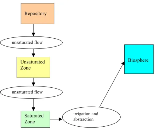
The conceptual model for leachate release in the ISAM Vault Safety Case consists of four parts, as shown in Figure 2.1.1.

Repository Unsaturated Zone Saturated Zone Biosphere unsaturated flow unsaturated flow irrigation and abstraction

Figure 2.1.1 Sub-Models in the Vault Safety Case Assessment for Leachate Release.

Radionuclides are transported in unsaturated groundwater flow from the repository to the unsaturated zone and then to the saturated zone. The saturated zone includes a well from which water is abstracted and used for irrigation; this is the route for radionuclide

(16)

8

Table 2.1.1 Initial Inventory in the Waste.

Radionuclide Inventory disposed (Bq)

H-3 1E+15 Cs-137 8E+15

C-14 1E+13 U-234 5E+10

Ni-59 2E+10 U-238 5E+10

Ni-63 1E+15 Pu-238 2E+10

Sr-90 1E+14 Pu-239 3E+10

Tc-99 3E+10 Pu-241 6E+11

I-129 6E+9 Am-241 2E+10

Table 2.1.2 Radionuclide Decay Chains.

Head of chain Daughters

U-238 U-234→ Th-230→ Ra-226→ Pb-210→ Po-210 Pu-238 U-234→ Th-230→ Ra-226→ Pb-210→ Po-210 Pu-239 U-235→ Pa-231→ Ac-227

(17)

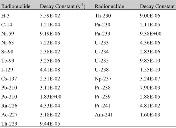
Table 2.1.3 Radionuclide Decay Constants.

Radionuclide Decay Constant (y-1) Radionuclide Decay Constant (y-1)

H-3 5.59E-02 Th-230 9.00E-06

C-14 1.21E-04 Pa-230 2.11E-05

Ni-59 9.19E-06 Pa-233 9.38E+00

Ni-63 7.22E-03 U-233 4.36E-06

Sr-90 2.38E-02 U-234 2.83E-06

Tc-99 3.25E-06 U-235 9.85E-10

I-129 4.41E-08 U-238 1.55E-10

Cs-137 2.31E-02 Np-237 3.24E-07

Pb-210 3.11E-02 Pu-238 7.90E-03

Po-210 1.83E+00 Pu-239 2.88E-05

Ra-226 4.33E-04 Pu-241 4.81E-02

Ac-227 3.18E-02 Am-241 1.60E-03

(18)

10

2.2 The Repository Sub-Model

The model compartments in this sub-model are shown in Figure 2.2.1. Radionuclides are leached from the waste into the concrete base and are then transported vertically in unsaturated flow to the unsaturated zone of the geosphere.

Waste

Concrete Base leaching

unsaturated flow

Figure 2.2.1 Compartments in the Repository Sub-Model.

The leaching rate from the waste in the repository depends on the flow rate through the waste and the physical and chemical properties of the waste and concrete base.

Leaching occurs once the drums containing the waste fail.

For a given radionuclide, the net transfer (leaching) rate (y-1), λleach, is:

R D q D R q w In Adv leach ϑ λ = = 2.2.1

where qAdv is the advective velocity of water (m y-1), qIn is the Darcy velocity of water

through the medium (m y-1) (equivalent to the infiltration rate), _ϑw is the water filled

porosity (-) of the medium, D is depth of the medium through which the radionuclide is transported (m), and R is the retardation coefficient (-) given by:

w Kd R ϑ ρ + = 1 2.2.2

(19)

where _ρ is the bulk density of the medium (kg m-3) and Kd is the sorption coefficient of the medium (m3 kg –1).

qIn and Kd are time dependent. A piece-wise constant performance of the cap covering

the waste is assumed. It is also assumed that chemical degradation of the concrete base is linear, starting at closure (undegraded) and lasting until 1000 years after closure (totally degraded). Chemical degradation is represented by varying the Kd values linearly between the initial and degraded values.

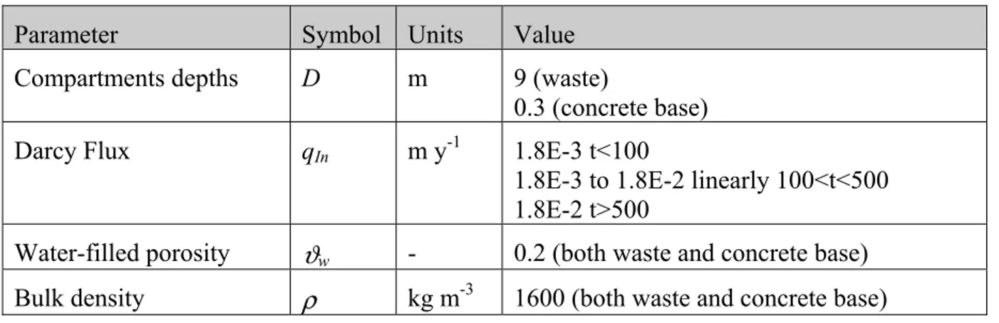
Relevant model parameter values are given in Tables 2.2.1 and 2.2.2.

Table 2.2.1 Parameter Values for the Repository Sub-Model. Parameter Symbol Units Value Compartments depths D m 9 (waste)

0.3 (concrete base) Darcy Flux qIn m y-1 1.8E-3 t<100

1.8E-3 to 1.8E-2 linearly 100<t<500 1.8E-2 t>500

Water-filled porosity _ϑ_w - 0.2 (both waste and concrete base) Bulk density _ρ kg m-3 1600 (both waste and concrete base)

(20)

12

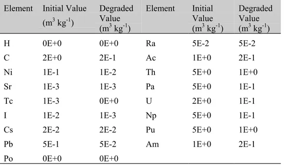
Table 2.2.2 Sorption Coefficients for the Repository Sub-Model. Element Initial Value

(m3 kg-1) Degraded Value (m3_kg-1₎ Element Initial Value (m3_kg-1₎ Degraded Value (m3_kg-1₎

H 0E+0 0E+0 Ra 5E-2 5E-2

C 2E+0 2E-1 Ac 1E+0 2E-1

Ni 1E-1 1E-2 Th 5E+0 1E+0

Sr 1E-3 1E-3 Pa 5E+0 1E-1

Tc 1E-3 0E+0 U 2E+0 1E-1

I 1E-2 1E-3 Np 5E+0 1E-1

Cs 2E-2 2E-2 Pu 5E+0 1E+0

Pb 5E-1 5E-2 Am 1E+0 2E-1

(21)

2.3 The Unsaturated Geosphere Sub-Model

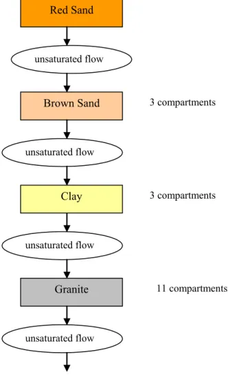
The model compartments in this sub-model are shown in Figure 2.3.1. The four strata in the unsaturated zone are here referred to simply as ‘Red Sand’, ‘Brown Sand’, ‘Clay’ and ‘Granite’. Radionuclides are transported in unsaturated groundwater flow from the Red Sand, to Brown Sand to Clay to Granite and then to the saturated zone of the geosphere. For simplicity the compartments that make up the different strata are not shown explicitly; in total there are 18 compartments in this sub-model.

Red Sand Brown Sand Clay Granite 3 compartments 3 compartments 11 compartments unsaturated flow unsaturated flow unsaturated flow unsaturated flow

Figure 2.3.1 Compartments in the Unsaturated Geosphere Sub-Model.

(22)

14

Table 2.3.1 Parameter Values for the Unsaturated Zone Sub-Model. Layer Depth D (m) Water-filled

porosity _ϑw Bulk density _ρ (kg m-3) Red Sand 2.7 0.2 1989 Brown Sand 8.5 0.2 2230 Clay 8.0 0.2 2160 Granite 35.8 0.2 1683

Table 2.3.2 Sorption Coefficients for the Unsaturated Zone Sub-Model. Element Red Sand

(m3 kg-1) Brown Sand (m3 kg-1) Clay (m3 kg-1) Granite (m3 kg-1)

H 0E+0 0E+0 0E+0 0E+0

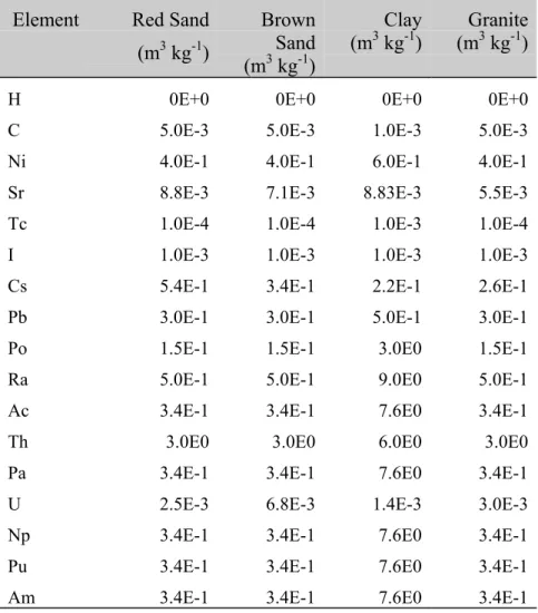
C 5.0E-3 5.0E-3 1.0E-3 5.0E-3 Ni 4.0E-1 4.0E-1 6.0E-1 4.0E-1 Sr 8.8E-3 7.1E-3 8.83E-3 5.5E-3 Tc 1.0E-4 1.0E-4 1.0E-3 1.0E-4 I 1.0E-3 1.0E-3 1.0E-3 1.0E-3 Cs 5.4E-1 3.4E-1 2.2E-1 2.6E-1 Pb 3.0E-1 3.0E-1 5.0E-1 3.0E-1 Po 1.5E-1 1.5E-1 3.0E0 1.5E-1 Ra 5.0E-1 5.0E-1 9.0E0 5.0E-1 Ac 3.4E-1 3.4E-1 7.6E0 3.4E-1 Th 3.0E0 3.0E0 6.0E0 3.0E0 Pa 3.4E-1 3.4E-1 7.6E0 3.4E-1 U 2.5E-3 6.8E-3 1.4E-3 3.0E-3 Np 3.4E-1 3.4E-1 7.6E0 3.4E-1 Pu 3.4E-1 3.4E-1 7.6E0 3.4E-1 Am 3.4E-1 3.4E-1 7.6E0 3.4E-1

(23)

2.4 The Saturated Geosphere Sub-Model

The model compartments in this sub-model are shown in Figure 2.4.1. There are nine Aquifer compartments together with a well compartment that is identical in structure to the other aquifer compartments. For simplicity only four of the total of ten compart-ments are shown in the Figure. Radionuclides are transported by saturated groundwater flow, and dispersion is represented as a diffusion-like process with the combination of 'forward' and 'backward' transfers between compartments giving the required

radionuclide flux.

Water is taken from the well for irrigation and other purposes, represented by the two transfers shown in Figure 2.4.1.

Aquifer 1 saturated flow dispersion Aquifer 2 Aquifer 9 Well irrigation dispersion saturated flow other abstraction

Figure 2.4.1 Compartments in the Saturated Geosphere Sub-Model.

In the saturated zone the Darcy velocity (q, in m y-1) of the groundwater is calculated from the hydraulic conductivity of the medium (K, in m y-1_{) and the hydraulic gradient}

(24)

16

There are three transfers associated with each compartment: Advective flux from

compart-ment i to compartcompart-ment j L R q i w ij A _ϑ λ , = 2.4.2 Forward dispersion (i to j) Aij x x ij D a , , λ λ ∆ = 2.4.3 Backward dispersion (j to i) Aji x x ji D a , , λ λ ∆ = 2.4.4

where _λA,ij is the rate of transfer of a contaminant by advection from compartment i to j

(y-1). _λD, ij is the rate of transfer of a contaminant by dispersion from compartment i to j

(y-1) with _∆X is the distance over which the gradient in radionuclide concentration is

calculated (m) and ax the dispersion length.

The transfer rate of radionuclides from the Well compartment due to irrigation (y-1), λirrig, is given by:

w w w irrig irrig R V d A ϑ λ = 2.4.5

where A is the area irrigated (m2), dirrig is the depth of effective irrigation water applied

(m y1_),_ϑ

w is the water filled porosity (-) of the saturated zone from which the water is

abstracted, Vw is the volume of the compartment representing the well (m3), and Rw is

the retardation coefficient (-) of the saturated zone (well).

The transfer rate of radionuclides due to abstraction of water for other purposes (y-1), λnon-irrig, is given by:

w w w irrig non irrig non R V V ϑ λ − − = 2.4.6

where Vnon-irrig is the volume of water abstracted for non-irrigation purposes plus loss

due to interception and evaporation (m3 y-1).

(25)

Table 2.4.1 Parameter Values for the Saturated Zone Sub-Model.

Parameter Symbol Units Value

Lengths of each compartment L = ∆X m 30

Volumes of each compartment V m3 90 Hydraulic Conductivity K m y-1 1.8E3

Hydraulic gradient _∂H/∂x - 0.1

Water-filled porosity _ϑw - 0.25

Bulk density _ρ kg m-3 2000

Dispersion length ax m 30

Area irrigated A m2 1E5

Irrigation depth dirrig m 0.05

Volume of water extracted for other purposes Vnon-irrig m3 3300

Table 2.4.2 Sorption Coefficients for the Saturated Zone Sub-Model. Element Kd (m3 kg-1) Element Kd (m3 kg-1) H 0E+0 Ra 5.0E-1 C 5.0E-3 Ac 3.4E-1 Ni 4.0E-1 Th 3.0E+0 Sr 5.5E-3 Pa 3.4E-1 Tc 1.0E-4 U 3.0E-3 I 1.0E-3 Np 3.4E-1 Cs 2.6E-1 Pu 3.4E-1 Pb 3.0E-1 Am 3.4E-1 Po 1.5E-1

(26)

(27)

3 AMBER and Ecolego Calculations

The original ISAM AMBER model was reviewed and an implementation error in the repository sub-model was found which was corrected. Revised AMBER calculations were undertaken for the intercomparison exercise with Ecolegoo.

3.1 Radionuclide Fluxes from the Repository

The first set of comparisons is for the flux of radionuclides from the repository sub-model into the unsaturated zone sub-sub-model.

Radionuclide fluxes were calculated at fixed times: 150, 300, 1000 and 10 000 years. In addition, the time and magnitude of the peak flux was calculated for each radionuclide. Table 3.1.1 gives the details of these calculations. Fluxes calculated at specified times are quoted to four significant figures, whilst the time and magnitude of the peaks are quoted to just two significant figures because it is not straightforward to identify the exact location of the peak and the peak fluxes can therefore be expected to be less accurately calculated than fluxes a specified times.

The fluxes for the seven radionuclides that give the highest peak fluxes are shown in Figure 3.1.1. For these radionuclides, this figure is similar to Figure 6.2 in IAEA

(2001), but is not exactly the same because more output times have been employed, and because of the error in the original ISAM calculations previously referred to.

It is not straightforward to provide an indication of the accuracy to be expected in the AMBER calculations. There is a global accuracy parameter of 1E-4 that is applied to the calculated compartment contents which can not be altered by the user. The calculated amount of a given radionuclide in any compartment will be accurate to at least 1E-4 times the maximum amount that has been calculated to be present in any compartment up to that time. This means that for radionuclides whose activities have been substantially reduced by radioactive decay, calculated amounts and fluxes can be expected to be less accurately calculated than radionuclides where radioactive decay has not significantly reduced activities.

Comparison of the AMBER and Ecolego calculations in Table 3.1.1 shows that agreement is generally excellent. In particular:

• The calculated peak fluxes and the times of the peaks agree to two significant figures.

• The calculated fluxes at specified times generally agree to at least three significant figures.

(28)

20

• Fluxes at 1000 years where rapid change in the radionuclide fluxes can be seen due to the end of the concrete degradation period. Fluxes calculated by Ecolego are slightly less than those calculated by AMBER. It is not clear which of the two sets of calculations is the more accurate.

(29)

21 100 0 100 00 100 000 100 00 00 Time ( Y e ar s) H3 C14 Ni63 Sr90 Tc9 9 Cs 137 Po21 0 Fluxes from the Repository.

(30)

22

Table 3.1.1 Fluxes from the Repository (AMBER calculations are in normal font;

Ecolego calculations are in italic font).

Radionuclide Flux at 150 y (Bq y-1₎ Flux at 300 y_{(Bq y}-1₎ Flux at_{1000 y} (Bq y-1₎ Flux at 10 000 y (Bq y-1₎ Peak

(Bq y-1₎ Peak_{Time (y)}

H-3 4.161E8 4.125E8 1.551E5 1.527E5 -3.257E-15 - 9.1E8 9.0E8 120 120 C-14 2.496E2 2.496E2 6.942E2 6.942E2 2.257E6 2.236E6 1.477E7 1.477E7 1.9E7 1.9E7 5600 5700 Ni-59 2.022E2 2.022E2 5.640E3 5.640E3 1.357E6 1.345E6 7.461E5 7.461E5 2.2E6 2.2E6 1700 1700 Ni-63 3.428E6 3.428E6 3.242E6 3.242E6 5.013E7 4.963E7 -1.188E-21 7.1E7 7.1E7 500 500 Sr-90 1.517E8 1.516E8 4.08E7 4.085E7 2.391E0 2.355E0 - 1.7E8 1.7E8 170 170 Tc-99 2.070E6 2.070E6 2.189E7 2.189E7 2.878E7 2.853E7 - 4.3E7 4.3E7 500 500 I-129 5.832E3 5.833E3 1.438E5 1.438E5 5.294E6 5.248E6 2.404E2 2.401E2 5.3E6 5.3E6 1000 1000 Cs-137 4.771E7 4.768E7 3.043E7 3.041E7 3.325E1 3.289E1 - 6.2E7 6.2E7 190 190 U-234 1.292E0 1.292E0 3.729E1 3.729E1 3.204E4 3.143E4 5.551E5 5.551E5 5.6E5 5.6E5 10 000 10 000 U-238 1.291E0 1.292E0 3.729E1 3.729E1 3.204E4 3.143E4 5.551E5 5.551E5 5.6E5 5.6E5 10 000 10 000 Pu-238 2.410E-2 2.410E-2 2.012E-1 2.012E-1 1.163E-1 1.158E-1 - 3.7E-1 3.7E-1 500 500 Pu-239 1.177E-1 1.177E-1 3.200E0 3.200E0 4.572E2 4.552E2 8.253E3 8.253E3 1.1E4 1.1E4 22 000 22 000 Pu-241 1.739E-3 1.730E-3 3.494E-5 3.468E-5 -1.114E-17 - 1.8E-3 1.8E-3 140 140 Am-241 3.145E0 3.145E0 6.754E1 6.754E1 3.133E3 3.119E3 2.276E-2 2.267E-2 3.6E3 3.6E3 1300 1300 Th-230 3.259E-4 3.259E-4 2.021E-2 2.021E-2 1.133E1 1.128E1 3.824E3 3.825E3 1.9E4 1.9E4 8.9E4 8.9E4 Ra-226 4.879E-02 4.880E-02 3.197E+00 3.197E+00 4.189E+02 4.189E+02 6.838E+04 6.838E+04 3.6E5 3.6E5 9.1E4 9.1E4 Po-210 1.077E+02 1.077E+02 3.878E+03 3.879E+03 2.521E+05 2.522E+05 2.779E+07 2.779E+07 1.4E8 1.4E8 9.1E4 9.1E4 Pb-210 2.509E-03 2.509E-03 3.085E-01 3.085E-01 4.122E+02 4.083E+02 6.827E+04 6.827E+04 3.6E5 3.6E5 9.1E4 9.1E4

(31)

Radionuclide Flux at 150 y (Bq y-1₎ Flux at 300 y_{(Bq y}-1₎ Flux at_{1000 y} (Bq y-1₎ Flux at 10 000 y (Bq y-1₎ Peak

U-235 1.042E-07 1.042E-07 5.594E-06 5.595E-06 1.596E-02 1.566E-02 2.468E+00 2.468E+00 6.8E0 6.8E0 5.1E4 5.1E4 Pa-231 3.921E-11 3.922E-11 4.957E-9 4.957E-9 1.299E-4 1.243E-4 2.783E-1 2.784E-1 3.7E0 3.7E0 8.5E4 8.6E4 Ac-227 2.725E-10 2.725E-10 2.703E-8 2.703E-8 5.917E-5 5.899E-5 1.386E-1 1.386E-1 1.8E0 1.8E0 8.5E4 8.6E4 Np-237 1.049E-05 1.049E-05 6.691E-04 6.691E-04 2.795E+00 2.674E+00 8.953E+01 8.953E+01 9.0E1 9.0E1 1.0E4 1.0E4 U-233 1.190E-08 1.188E-08 1.357E-06 1.356E-06 1.001E-02 9.871E-03 3.587E+00 3.587E+00 1.1E1 1.1E1 6.9E4 6.9E4 Th-229 1.376E-11 1.374E-11 3.459E-9 3.455E-9 1.848E-5 1.840E-5 1.147E-1 1.147E-1 1.1E0 1.1E0 8.1E4 8.0E4

(32)

24

3.2 Radionuclide Fluxes from the Unsaturated Zone

The second set of comparisons is for the flux of radionuclides from the unsaturated zone sub-model into the saturated zone sub-model.

Radionuclide fluxes were calculated at fixed times: 300, 1000 and 10 000 years (there is no significant flux for any radionuclide at 150 years). In addition, the time and

magnitude of the peak flux was calculated for each radionuclide. Table 3.2.1 gives the details of these calculations. Fluxes are presented to the same number of significant figures as previously.

The fluxes for the four radionuclides that give the highest peak fluxes are shown in Figure 3.2.1. For these radionuclides, this figure is similar to Figure 6.4 in IAEA (2001), but is not exactly the same because of the previously noted differences. Comparison of the AMBER and Ecolego calculations in Table 3.1.1 shows that agreement is generally excellent. In particular:

• The calculated fluxes at specified times generally agree to around three significant figures, except for H-3 for the reasons discussed in Section 3.1.

(33)

25 1 00 0 1 00 00 10 000 0 10 00 000 Time (Yea rs ) C14 Tc9 9 I1 29 U238 Fluxes from

(34)

26

Table 3.2.1 Fluxes from the Unsaturated Zone (AMBER calculations are in normal font; Ecolego calculations are in italic font).

Radionuclide Flux at 300 y

(Bq y-1₎ Flux at 1000 y_{(Bq y}-1₎ Flux at_{10 000 y}

(Bq y-1₎

Peak

H-3 4.805E-7 4.770E-7 1.351E-12 1.030E-12 - 7.9E-4 7.8E-4 5.0E2 5.0E2 C-14 - -3.236E-17 7.914E2 7.924E2 7.9E5 7.9E5 2.9E4 2.9E4 Ni-59 - - - 1.4E-2 1.4E-2 1.0E6 1.0E6 Ni-63 - - - - -Sr-90 - - - - -Tc-99 8.785E-13 8.896E-13 3.115E+04 3.118E+04 1.691E+00 1.635E+00 1.9E7 1.9E7 2.5E3 2.5E3 I-129 - 1.792E-06 1.805E-06 5.740E+05 5.742E+05 1.4E6 1.4E6 7.4E3 7.5E3 Cs-137 - - - - -U-234 - -1.254E-17 6.918E+02 6.924E+02 5.1E5 5.1E5 3.5E4 3.5E4 U-238 - -1.253E-17 6.917E+02 6.923E+02 5.1E5 5.1E5 3.5E4 3.5E4 Pu-238 - - - - -Pu-239 - - - 4.7E-12 4.7E-12 5.1E5 5.2E5 Pu-241 - - - - -Am-241 - - - - -Th-230 - - 4.835E-03 4.843E-03 2.0E2 2.0E2 1.2E5 1.2E5 Ra-226 - - 6.678E-03 6.694E-03 1.2E3 1.2E3 1.2E5 1.2E5 Po-210 - - 2.124E-02 2.129E-02 4.0E3 4.0E3 1.2E5 1.2E5 Pb-210 - - 1.063E-02 1.066E-02 2.0E3 2.0E3 1.2E5 1.2E5 U-235 - - 6.735E-04 6.743E-04 7.0E0 7.0E0 7.2E4 7.2E4 Pa-231 - - 9.232E-08 9.251E-08 4.8E-2 4.8E-2 1.2E5 1.2E5 Ac-227 - - 8.906E-08 8.925E-08 4.8E-2 4.8E-2 1.2E5 1.2E5

(35)

Radionuclide Flux at 300 y

(Bq y-1₎ Flux at 1000 y_{(Bq y}-1₎ Flux at_{10 000 y}

(Bq y-1₎

Peak

Np-237 - - - 1.2E-4 1.2E-4 1.0E6 1.0E6 U-233 1.052E-03 1.054E-03 3.3E1 3.3E1 1.7E5 1.7E5 Th-229 6.665E-08 6.680E-08 3.5E-2 3.5E-2 1.9E5 1.9E5

(36)

28

3.3 Well Water Concentrations

The third set of comparisons is for the concentration of radionuclides in well water in the saturated zone sub-model.

Radionuclide concentrations were calculated at fixed times: 1000 and 10 000 years (there are no concentrations for any radionuclide at 150 or 300 years). In addition, the time and magnitude of the peak concentration were calculated for each radionuclide. Table 3.3.1 gives the details of these calculations. Concentrations are presented to the same number of significant figures as previously.

The concentrations for the four radionuclides that give the highest peak fluxes are shown in Figure 3.3.1; these are the same radionuclides that gave the highest peak fluxes from the unsaturated zone in Section 3.2. For these radionuclides, this figure is similar to Figure 6.6 in IAEA (2001), but is not exactly the same because of the previously noted differences.

Comparison of the AMBER and Ecolego calculations in Table 3.3.1 shows that agreement is generally excellent. In particular:

• The calculated fluxes at specified times generally agree to around three significant figures.

This degree of agreement between the two sets of calculations is impressive given the large number of compartments in the model and the inclusion of decay chains with up to six members.

(37)

29 1 00 0 1 00 00 100 00 0 10 00 000 Time (Yea rs ) C14 Tc9 9 I12 9 U238 W ell W ater Concentr ation s.

(38)

30

Table 3.3.1 Well Water Concentrations (AMBER calculations are in normal font;

Ecolego calculations are in italic font).

Radionuclide Conc. at 1000 y

(Bq m-3₎ Conc. at 10 000 y_{(Bq m}-3₎ Peak_{(Bq m}-3₎ Peak_{Time (y)}

H-3 -2.616E-11 -1.230E-12 -9.3E-8 -5.0E2 C-14 - 9.360E-02 9.372E-02 9.5E1 9.5E1 2.9E4 2.9E4 Ni-59 - - 1.7E-6 1.7E-6 1.0E6 1.0E6 Ni-63 - - - -Sr-90 - - - -Tc-99 3.719E+00 3.723E+00 2.040E-04 1.973E-04 2.2E3 2.2E3 2.5E3 2.5E3 I-129 2.008E-10 2.023E-10 6.929E+01 6.932E+01 1.7E2 1.7E2 7.4E3 7.5E3 Cs-137 - - - -U-234 - 8.253E-02 8.260E-02 6.2E1 6.2E1 3.5E4 3.5E4 U-238 - 8.251E-02 8.259E-02 6.2E1 6.2E1 3.5E4 3.5E4 Pu-238 - - - -Pu-239 - - -5.5E-16 -5.2E5 Pu-241 - - - -Am-241 - - - -Th-230 - 5.771E-07 5.781E-07 2.4E-2 2.4E-2 1.2E5 1.2E5 Ra-226 - 7.961E-07 7.979E-07 1.4E-1 1.4E-1 1.2E5 1.2E5 Po-210 - 2.532E-06 2.538E-06 4.8E-1 4.8E-1 1.2E5 1.2E5 Pb-210 - 1.267E-06 1.270E-06 2.4E-1 2.4E-1 1.2E5 1.2E5 U-235 - 8.029E-08 8.039E-08 8.4E-4 8.4E-4 7.2E4 7.2E4 Pa-231 - 1.101E-11 1.103E-11 5.8E-6 5.8E-6 1.2E5 1.2E5

(39)

Radionuclide Conc. at 1000 y

(Bq m-3₎ Conc. at 10 000 y_{(Bq m}-3₎ Peak_{(Bq m}-3₎ Peak_{Time (y)}

Ac-227 - 1.062E-11 1.064E-11 5.8E-6 5.8E-6 1.2E5 1.2E5 Np-237 - - 1.5E-8 1.5E-8 1.0E6 1.0E6 U-233 - 1.253E-07 1.255E-07 4.0E-3 4.0E-3 1.7E5 1.7E5 Th-229 - 7.947E-12 7.965E-12 4.2E-6 4.2E-6 1.9E5 1.9E5

(40)

(41)

4 Conclusions

The most important situation where agreement may not be as good as that generally found is where radionuclides have been subject to substantial losses due to radioactive decay; at times after the production of the radionuclide that are very much greater than the radionuclide half-life.

(42)

(43)

References

Avilia, R, Broed R. and Pereira, A (2003). Ecolego - a Toolbox for Radioecological Risk Assessments. International Conference on the Protection of the Environment from the Effects of Ionising Radiation, 6 –10 October 2003, Stockholm, Sweden.

Enviros and Quintessa Ltd (2003). AMBER version 4.5.

IAEA (2001). ISAM, The International Programme for Improving Long Term Safety Assessment Methodologies for Near Surface Radioactive Waste Disposal Facilities: Vault Safety Case Report. ISAM Document version 1.3, August 2001: working material.

SKB (1999). Deep Repository for Spent Fuel. SR97- Post-closure safety, volumes I and II. SKB report TR-99-06.

SKI and SSI (2003). AMBER and Ecolego Intercomparisons using Calculations from SR97.

(44)

(45)

(46)

S T A T E N S K Ä R N K R A F T I N S P E K T I O N

Swedish Nuclear Power Inspectorate

POST/POSTAL ADDRESS SE-106 58 Stockholm BESÖK/OFFICEKlarabergsviadukten 90 TELEFON/TELEPHONE +46 (0)8 698 84 00 TELEFAX +46 (0)8 661 90 86

E-POST/E-MAIL ski@ski.se WEBBPLATS/WEB SITEwww.ski.se