1
New model for predicting customer lifetime
value in the B2B Telecom Industry
In the B2B Telecom Industry the customer-firm relationship results in a cash flow structure with interesting properties. Initially there is a large customer acquisition cost (CAC) emerging from the sales process and the marketing efforts. Thereafter the firm will service the customers, generating frequent small positive net cash flows. However, it is crucial for overall profitability that the customers stay long enough for the monthly payments to exceed the CAC and the monthly costs associated with servicing the customer. Since the average lifetime of the customers in the B2B Telecom industry is long it is not always possible to observe how long customers from a certain segment is going to stay when evaluating the segment’s potential profitability. Therefore it is useful to be able to predict the average customer’s lifetime. Previous existing models have not been able to take into consideration that customers can be bound with a contract to stay a certain period, but research at Faculty of Engineering at Lund University resulted in a new model with this capability.
In the short perspective, the cash flow structure of a customer with an initial CAC and subsequent small net positive cash flows will generate large negative cash flows during an expansion of customer base. The reason is that the new part of the customer base will not yet compensate for the repeated CACs. Therefore it is important for companies with this type of individual customer cash flow structure to be prepared with enough cash when expanding to avoid defaulting. To decrease the capital required for an expansion it is most effective to improve the cost effectiveness of the CAC.
In the long run the customers’ cash flows has to be discounted as money is worth more today compared to in the future. This gives rise to the expression Customer Lifetime Value (CLV) – the discounted value of past and future cash flows associated with a customer. The CLV of all current and future customers can be used as a proxy to evaluate the firm’s total value - CLV is an important metric! While CAC was the most important factor in the short term, it is retention (the probability of a customer retaining with the firm, which is a metric containing the information of the lifetime) that is most significant in the long term by affecting the CLV the most. Therefore the most crucial part of the problem of predicating the CLV is solved if one can predict the retention. It is also argued that it is the most difficult variable of CLV to predict.
It was until recently not possible to model the rate of which customers are leaving (churning) in the B2B Telecom industry. The reason was that the customers were bound with contract, which changed their behaviour in a way that did not fit previous models. The previous models assumed that the retention rate (probability that a customer will stay) of an individual customer was constant and independent of the age of the customer. However, since customers are bound in the B2B telecom industry for long periods of time this must be taken into consideration in the model as naturally a customer which is bound will most likely be more inclined to retain compared to a customer which is not bound. The current existing data of how customer has
Customer lifetime value (CLV) -
The discounted value of past and future cash flows associated with a customer.
Churn rate – rate at which
customers are leaving.
Retention rate – probability that a
customer will stay. Retention rate + churn rate = 1.
Boundtime – the duration the
2
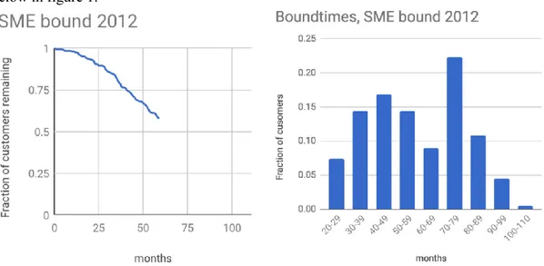
remained with respect to time up until now with its distribution of boundtimes is displayed below in figure 1.Figure 1. Displays the existing data of fraction of customers remaining with respect to time (left) and the customers’ current corresponding boundtimes i.e. the distribution of for how long the customers are bound. “SME bound” in the title of the graphs refers to the specific segment in question and “2012” refers to the year the customers signed up.
The proposed model assumes that each customer is in either of three states as shown in table 1. The states are: “Alive and dormant” which signifies the time the customer is still a customer and does not consider leaving thus having retention 1 (probability of remaining = 1), “Alive and awake” when the customer is still a customer but does consider leaving with probability between 0 and 1 at each instant, and “Dead” when a customer has churned. The previous models had only two states; dead and alive with no distinction between if a customer was bound or not.
Table 1. Displays the proposed possible three states of a customer.
Customer state Retention
Alive and dormant 1
Alive and awake Between 0 and 1
Dead -
The task now at hand is to determine when each customer goes from state “Alive and dormant” to “Alive and awake”. At first thought it seem reasonable to assume that each customer transitions when the bound contract expires. However, there is a probability that the customer starts considering leaving before the expiry date since: 1) there is a risk that it considers the benefits of leavening outweighs the costs of remaining (most likely near the end of the contract expiry date) and 2) there is a risk that the customer will default, forcing a termination of the contract with Telavox. Due to these factors it is not possible to assume that the customers become awake exactly when their contracts end. What makes it even more difficult is that the current boundtimes displayed in figure 1 are not final; each customer can update their boundtime as they remain a customer. These uncertainties make it difficult to know the final awakening distribution. Therefore it is part of the model to vary the awakening distribution and at each case find the retention of the customers when alive and awake. This will in turn generate many different extrapolations. By finding the area under the graphs it is possible for each case to find the expected lifetime of the customer. By calculating the average of these expected lifetimes it is possible to find a single proposed value of the expected lifetime of a customer. An example of an extrapolation of the data from figure 1 is displayed in figure 2.
3
Figure 2. Displays the resulting extrapolation using an awakening distribution with mean 55 and standard deviation of 40 that is assumed to follow a normal distribution.Even if the resulting models that extrapolate the data always fit the data at hand it is not a guarantee that the model will generate the true future fraction of customers remaining with respect to time. Therefore the main focus for future research must be to acquire a dataset with more complete time series (i.e. data of groups of customers where almost all customers has had time to churn) and then test if the model is any good at predicting the future. Up until then this model shall only be considered a proposal. However, the model is still useful as it gives an educated estimate of the average lifetime of a group of customers, which was not possible to find before.