Evaluation of a sleepiness warning system : a test truck study

Full text

(1)VTI notat 9A-2009 Published 2009. www.vti.se/publications. Evaluation of a sleepiness warning system a test track study Anna Anund Magnus Hjälmdahl.

(2)

(3) Foreword This study has been done in collaboration between the EU project SENSATION and the national project DROWSI. I would like to thank all those that contributed to the project, especially Beatrice Söderström responsible for the participants, Sven-Åke Linden co-driver through all nights, Harry Sörensen responsible for equipping the car and for support during the analysis of data and Magnus Hjälmdahl for valuable discussions and support through all phases of the study. Last but not least I would like to thank all 40 participants that made this study possible to perform. January, 2009 Anna Anund. VTI notat 9A-2009 Dnr: 2006/0165-26.

(4) Quality review External peer review was performed on 20 October 2008 at VTI by Sverker Almqvist. Anna Anund has made alterations to the final manuscript of the report. The research director of the project manager, Jan Andersson, examined and approved the report for publication on 3 February 2009.. VTI notat 9A-2009.

(5) Table of contents List of Figures..................................................................................................... 5 List of Tables ...................................................................................................... 7 Glossary ............................................................................................................. 8 Summary ............................................................................................................ 9 Sammanfattning ............................................................................................... 11 1 1.1 1.2. Introduction ............................................................................................ 13 SENSATION warning concept ............................................................... 13 SENSATION hypo vigilance management system (HVMS)................... 14. 2 2.1 2.2. Aim and hypothesis ............................................................................... 16 Aim ........................................................................................................ 16 Hypothesis ............................................................................................. 16. 3 3.1 3.2 3.3 3.4 3.5. Method................................................................................................... 18 Design.................................................................................................... 18 Participants ............................................................................................ 18 Experimental settings............................................................................. 19 Scenario................................................................................................. 21 Procedure .............................................................................................. 21. 4 4.1 4.2 4.3 4.4 4.5 4.6 4.7. Results................................................................................................... 38 Participants background ........................................................................ 38 Experiences of the test .......................................................................... 41 Risk estimation/own capability ............................................................... 44 Received warnings ................................................................................ 45 Recognising the sensation of sleepiness ............................................... 47 Stopping driving/taking a break.............................................................. 48 Effectiveness ......................................................................................... 52. 5 5.1 5.2 5.3 5.4 5.5 5.6. Discussion ............................................................................................. 60 Recognizing the need for a break .......................................................... 60 HMI ........................................................................................................ 60 User acceptance.................................................................................... 61 Effectiveness ......................................................................................... 61 Negative behaviour adaptation .............................................................. 62 Methodological considerations............................................................... 62. 6. Conclusions ........................................................................................... 64. References ....................................................................................................... 65 Annexes. VTI notat 9A-2009.

(6) VTI notat 9A-2009.

(7) List of Figures Figure 1 Warning strategy (HVMS) developed with in SENSATION .......................... 15 Figure 2 Meilhaus ME-96 Computer I/O card, taking a 24V input. .............................. 15 Figure 3 Actiwrist and vibration unit used in the car application .................................. 15 Figure 4 The placement and design of the feedback to the driver. The lights were green, yellow, orange, or red depending on the output from the Siemens drowsiness algorithm (DMS) based on unobtrusive measures blink duration.................................. 18 Figure 5 Aerial view of Mantorp Park raceway ............................................................. 19 Figure 6 The instrumented vehicle ............................Fel! Bokmärket är inte definierat. Figure 7 A photo illustration the placement of the electrodes for the EOG measurments. The tape was placed on the electrodes to mask them so that the unobtrusive camera system (DMS) did not mistake them for eyes................................ 22 Figure 8 The Vitaport 2 digital recorder......................................................................... 24 Figure 9 The blink complex from start to stop is presented, in green the filtered vertical EOG derivate is seen, in read the un-derived filtered vertical EGO signal. Blink duration is marked in blue and closing an opening time in black. ....................... 25 Figure 10 The DMS camera and IR source .................................................................... 26 Figure 11 The ORS touch screen as it was mounted in the instrumented vehicle. (Uppmärksamhet = Awareness, Körning = driving behaviour, Blink = blink, Gäsp = yawn, Kroppsposition = body position, Kroppsrörelse = body movements, Varning = Warning)......................................................................................................................... 28 Figure 12 Resolution of ORS and indicators from the blink complex ........................... 29 Figure 13 Mean blink duration distributed by lap (laps with pauses have been excluded). Error bars represent SE. ................................................................................ 30 Figure 14 Mean ORS distributed by lap (laps with pauses have been excluded). Error bars represent SE................................................................................................... 30 Figure 15 Example of the tool for data fusion and interpolation of missing data for lateral position. ............................................................................................................... 32 Figure 16 The recalculation of the time-based analogue values to distance where = measured values and = calculated values. .................................................................... 33 Figure 17 The recalculation of the time-based digital values to distance where = measured values and = calculated values. ................................................................... 34 Figure 18 Time driven for each participant .................................................................... 36 Figure 19 ESS scores of the participants. ....................................................................... 39 Figure 20 The test drivers’ views on whether they had got enough sleep during the night before the test. ................................................................................................. 40 Figure 21 Drivers who had experienced incidents caused by fatigue/sleepiness. .......... 40 Figure 22 Participants’ opinions on how well they performed when driving? .............. 41 Figure 23 How strenuous an effort was needed to stay awake when driving? (Only the endpoints of the scale were defined.) ............................................................. 42. VTI notat 9A-2009. 5.

(8) Figure 24 How realistic was the test compared to real driving? (Only the endpoints of the scale were defined.).............................................................................................. 42 Figure 25 Average KSS reported before and after the driving session. Condition: 0=baseline, 1=early warning; 2=late warning; 3=feedback + late warning. .................. 43 Figure 26 Distribution of ORS levels on distance driven (1 value for every 5 metres) . 44 Figure 28 No difference between the three comparison groups is obvious (KruskalWallis one-way analysis of variance by ranks: χ2(2) = 2.57; p=.276). ............................ 50 Figure 29 No differences between the three comparison groups are obvious (Kruskal-Wallis one-way analysis of variance by ranks: χ2(2) = .221; p=.895).............. 51 Figure 30 No differences between the three comparison groups are obvious (Kruskal-Wallis one-way analysis of variance by ranks: χ2(2) = 2.56; p=.278).............. 51 Figure 31 Speed at the 50 km/h speed limit sign. Condition; 0= baseline; 1= early warning; 2=late warning; 3=feedback + late warning. ORS; 0=alert; 1=first signs of sleepiness; 2= Sleepy; 3=Severe sleepiness. Error bars=SE. ......................................... 53 Figure 32 Average speed over the 1000-1500 metre section (70 km/h); error bars represent standard error of mean (SE)............................................................................ 54 Figure 33 Average speed over the 2200-2500 metre section (70 km/h); error bars represent standard error of mean (SE)............................................................................ 55 Figure 34 Lateral position at traffic sign speed limit of 50 km/h. Condition; 0= baseline; 1= early warning; 2=late warning; 3=feedback + late warning. ORS; 0=alert; 1=first signs of sleepiness; 2= Sleepy; 3=Severe sleepiness Error bars=SE. ... 56 Figure 35 Mean number of breaks at traffic sign speed limit of 50 km/h, separated by condition at ORS level 0............................................................................................ 57 Figure 36 Mean number of breaks at traffic sign speed limit of 50 km/h, separated by condition at ORS level 1............................................................................................ 58 Figure 37 Mean number breaks at traffic sign speed limit of 50 km/h, separated by condition at ORS level 2................................................................................................. 59. 6. VTI notat 9A-2009.

(9) List of Tables Table 1 Description of the circuit (lap) and the position of the traffic signs with speed limits 50 -and 70 km/h.......................................................................................... 20 Table 2 The parameters stored in the resulting text file. ................................................ 25 Table 3 The content of the DMS logfile in terms of label, description, Unit and specific comments. ......................................................................................................... 26 Table 4 The four different drowsiness stage used by the Simens system (DMS) .......... 27 Table 5 Karolinska Sleepiness Scale, as modified by Reyner and Horn (1998). ........... 27 Table 6 Driving behaviour data recorded in the field trial ............................................. 31 Table 7 Total observations per participant. Grey marked participants were excluded from further analysis because their driving time did not reach the limit of 1.2 hours (4322 sec.). ..................................................................................................................... 35 Table 8 Observations – distance driven (selection of the first 1.2 hours driven) ........... 37 Table 9 Participants’ backgrounds with regard to driving experience, medication, and use of coffee, alcohol etc. ........................................................................................ 38 Table 10 Number of received warnings based on 1.2 hours’ driving (Source=ORS).... 45 Table 11 Drivers continuing driving - Observed body movements, changes in body position, or yawning. (Source: ORS) ............................................................................. 47 Table 12 Drivers continuing driving – opening the window, turning on the fan, cold air, etc., or stopping at the side of the track to open the window/door. (Source: Test leader’s notes) .......................................................................................... 47 Table 13 Drivers that stopped at the side of the track for a nap, or stopped at the laboratory (Source: Test leader’s notes)......................................................................... 48 Table 14 Question: Did the warning come at the right moment?................................... 49 Table 15 Question: What contributed most to your recognition of the warning? .......... 50 Table 16 Speed (km/h) – Differences in speed for different conditions. F-value; df and p-value (α=0.05) .................................................................................................. 54 Table 17 Differences between lateral position (cm) for the different conditions. F-value; df and p-value (α=.05)...................................................................................... 56 Table 18 Question: Is there a risk that the sleepy driver will keep on driving longer with an activated warning system like the one you have used ? ......................... 59. VTI notat 9A-2009. 7.

(10) Glossary DMS. (Driver monitoring system). EOG. (Electrooculogram). EEG. (Electroencephalogram). EMG. (Electromyogram). ESS. (Epworth sleepiness scale). GPS. (Global Positioning System). HMI. (Human Machine Interaction). HW. (Hard Ware). HVMS. (Hypovigilance management system). KSS. (Karolinska sleepiness scale). ORS. (Observer rating scale). SW. (Soft Ware). Vitaport. (Mobile recorder for physiological measures e.g. EOG). 8. VTI notat 9A-2009.

(11) Evaluation of a sleepiness warning system – a test track study By Anna Anund and Magnus Hjälmdahl VTI (Swedish National Road and Transport Research Institute) SE-581 95 Linköping Sweden. Summary Sleep related crashes have received increasing attention over the past decade. Driver support systems that are able to detect sleepiness and warn the driver could be a potential countermeasure to reduce sleepiness related crashes. The aim of this study was to evaluate a warning system in an experimental investigation performed in a real time car driving application. An additional aim was also to examine the suitability of using an experimental vehicle at test track for evaluation of a sleepiness warning system. The modalities used for warning was a combination of sound, vibrations in belt and spoken messages. In addition a hand worn confirmation button was used. In total 40 participants drove at a closed test track during night (00h–05h). They were instructed to sleep between 01.00 and 07.00 for two nights prior to the night of the experiment. The design of the study was a between group, with 10 participants in each group. The four different groups experienced one of the following: A: No warning – baseline; B: SENSATION warning system with an early trigger; C: SENSATION warning system with a late trigger; D: Feedback (DMS – Siemens) and warning with a late trigger. The trigger of the warnings was based on observer registrations of the driver and driver behaviour. The drivers were instructed to drive a distance of 110 kilometres. The car was a Volvo 850, equipped with sensors in order to measure driving behaviour (lateral position, speed, steering wheel angle). As sleepiness indicators blink duration was used (mean and sd), measured with EOG. After the drive the participants answered a questionnaire. The experiment focused on comprehension, usability, effectiveness, and acceptance. There was no significant observable difference between the groups that received the warning at an early point, at a late point, or at a late point in combination with a feedback system. Regarding the self reported measures, it should be noticed that no participant considered the warning to be too early. The sound was seen as most disturbing and most effective. The belt vibration was seen as least disturbing, but also as least effective. These results seem to be highly related to the level of the sound and the amplitude of the vibrations. In total, 27 out of 30 drivers in group B-D reported they had experienced warnings. About 50% felt that the warning had come at the correct time, and no driver found it to be too early. More than 70% stated that the warning had influenced their driving and 85% thought it had made them more awake; 55% stated that the warning had helped them to stay awake. The warning was easy to understand, and the drivers felt that it was clear what was expected from them. No clear feedback was given when pressing the confirmation button, and so some users pressed the button several times. Confirmation feedback to the user is necessary. Almost all drivers thought that the warning system would contribute to increased traffic safety, and that it would contribute to the prevention of crashes caused by sleepiness. Even if driving for real on a test track gives higher ecological validity than a driving simulator there is still problems to be solved. Drivers, prepared to be sleepy during night time will most truly accept and agree with a given warning. This will influence the drivers’ acceptance of the system. Additionally, sensors used do not have a high VTI notat 9A-2009. 9.

(12) technical reliability for speeds under 50 km /h. However, the present study shows that a test during real driving can be done without any risky situations. The recommendation is to take the next step and move out on real roads with experimental cars equipped with double commands in order to have a high external validity, but still a high control, at least regarding the participants’ preparation and actions under the experiment.. 10. VTI notat 9A-2009.

(13) Utvärdering av ett varningssystem för trötta förare – en studie genomförd på testbana av Anna Anund och Magnus Hjälmdahl VTI 581 95 Linköping. Sammanfattning Trötthetsrelaterade olyckor har fått ett ökat fokus under de senaste åren. Förarstöd för att detektera och varna trötta förare kan vara en potentiell åtgärd för att minska antalet trötthetsrelaterade olyckor. Syftet med föreliggande studie vara att utvärdera ett varningssystem för trötta förare. Utvärderingen har skett som ett experiment genomfört vid körning på riktigt väg med trötta förare. Ytterligare ett syfte var att utreda om försök med körning på testbana är en möjlig utvärderingsmetodik av varningssystem. Total deltog 40 personer. De körde på en testbana mellan klockan 00 och 05 på natten. De hade sovit 01–07 två nätter före försöksdagen. Studiens design var en mellangruppsdesign med 10 förare i varje grupp: A: ingen varning; B= SENSATION varningssystem med en tidig triggning: C= SENSATION varningssystem med en sen triggning; D=SENSATION varning med en sen triggning och med feedback till föraren avseende hans/hennes blink duration. Triggningen skedde baserat på en försöksledares systematiska bedömning genomförd med hjälp av en försöksledarskattning (ORS). Varningen som användes var en kombination av ljud, vibrationer och talade meddelanden. Förarna fick köra 110 kilometer i en Volvo 850. Bilen var utrustad med sensorer för att mäta förarens beteende (sidoläge, hastighet och rattvinkel). Som indikatorer för sömnighet användes blinkduration (medel- och standardavvikelse), mätt med EOG. Efter körningen fick försökspersonerna besvara en enkät. Experimentet fokuserade på förståelighet, användbarhet, effektivitet och acceptans. Resultaten visar att det inte fanns någon signifikant skillnad mellan grupperna som fick varning och de som inte fick varning. Förarna upplevde inte i något fall att varningen kom för tidigt. Ljudet var det som upplevdes som mest störande, men även mest effektivt. Bältesvibrationerna var de som upplevdes som minst störande men även som minst effektiva. Resultaten tenderar att vara relaterade till ljudnivån och amplituden i vibrationen. Totalt var det 27 av 30 förare i grupp B–D som rapporterade att de fått varningar. Cirka 50 procent ansåg att varningen kom korrekt i tid. Ingen ansåg att den kom för tidigt. Fler än 70 procent ansåg att varningen påverkade deras körning och 85 procent ansåg att den hjälpt dem att vara vakna. Varningarna upplevdes om enkla att förstå och att det var tydligt vad som förväntades av föraren. En del i varningssystemet var att föraren skulle bekräfta varningen genom att trycka på en armbandsburen knapp. Resultaten visade att förarna efterfrågade en bekräftelse på om tryckningen gått fram. Återkoppling till förare är viktigt och studien visade att förarna tryckte flera gånger då de var osäkra på om tryckningen gått fram. I stort sett upplevde alla förarna att systemet kommer att bidra till en ökad trafiksäkerhet och till att minska antalet sömnighetsrelaterade olyckor. Även om körning på riktigt på testbana har en hög ekologisk validitet, högre än i simulator, så återstår problem att lösa. Förare är förberedda för att köra på natten och kommer med stor sannolikhet att acceptera och hålla med om att en given varning är befogad. Det påverkar således studiens resultat avseende acceptans. Vidare ger en miljö som testbanan stora utmaningar för sensorerna. En stor del av körningen sker i låga VTI notat 9A-2009. 11.

(14) hastigheter och med kurvradier som överstiger det vi normalt ser. Studien visar dock att vi kan genomföra denna studie av sömniga förare utan att ge avkall på säkerheten. Vi rekommenderar att nästa steg blir att förlägga körningen på riktig väg i syfte att öka graden av ekologisk validitet och samtidigt behålla den höga graden av kontroll på förarnas förberedelser och körning.. 12. VTI notat 9A-2009.

(15) 1. Introduction. Sleep related crashes have received increasing attention over the past decade. The National Transportation and Safety Board of the USA has pointed out that sleepiness while driving is one of the most important reasons for road crashes (NTSB, 1999). Conservative official statistics show that about 1-3 percent of all crashes are sleep related (Åkerstedt & Kecklund, 2001; Pack et al., 1995). However, epidemiological studies based on self-report studies or in-depth crash investigations show much higher figures and suggest that, in fact, about 10 to 20 percent of all crashes might be sleep or fatigue related (Horne & Reyner, 1995a, 1995b; Maycock, 1997; Stutts, Wilkins, & Vaughn, 1999). Sleepiness is operationally defined as a physiological drive to sleep. This is the latent, fundamental type of sleepiness that in some cases can be masked by surrounding factors and in others can result in manifest sleepiness. From a driving point of view, sleepiness can be seen as the lack of ability to maintain a wakeful state of attention.. 1.1. SENSATION warning concept. Driver support systems that are able to detect sleepiness and warn the driver represent a means to reduce sleepiness -related crashes, and thus can help to increase safety and avoid tragedy. The EU project SENSATION, which aims to contribute to the increase of safety and the reduction of crashes, has for this reason developed an unobtrusive sleepiness warning system (here called HVMS that stands for hypovigilance management system). Relevant general functions and guidelines, along with a benchmark of existing systems, have been used during the development and it was concluded that there was only one working system known to the authors which takes an integrative approach with respect to these three topics, namely the AWAKE system ((Bekiaris, Nicolaou, & Peters, 2003). During the development of the SENSATION system, the following criteria were kept in mind: Attention: There is a need for new and innovative human-machine-interaction concepts for HVMS that are guaranteed to draw the attention of the hypovigilant user, but are also guaranteed not to scare or surprise the user, in order to avoid aversive reactions which could cause an even worse situation. Universality: The user must be warned efficiently with respect to the context and task in all of the potential application scenarios. However, given the many potential application fields, it would require an enormous technical effort to design a specific HMI for every application. Thus, one goal of the SENSATION project is to define the smallest possible set of Human Machine Interaction (HMI) elements which still satisfies these requirements, along the lines of a tool kit. Usability: The HVMS will have a wide application only if a good usability is achieved. In the context of this work, at least two aspects of usability should be addressed. On the one hand, the system must not disturb the main task or work task of the user, for example driving a car or operating machines. On the other hand, the HMI must be unobtrusive and reliable. One way to meet the latter requirement is to integrate the HMI into everyday items, clothes, or work clothes. Unobtrusiveness: Further research might lead to solutions such as Bluetooth driven, vibrating or contracting rings, earrings, glasses, or even clothes. VTI notat 9A-2009. 13.

(16) Subproject 4 of the SENSATION project has developed a hypovigilance warning system. One major part of this system is the warning strategy and the accompanying HMI devices. This system was used in the DROWSI pilot performed on the Mantorp Park test track, and is presented in this deliverable.. 1.2. 1.2 SENSATION hypo vigilance management system (HVMS). The warning strategy of the HVMS is in accordance with the outline of the basic sequence of the human–machine communication. Five hypovigilance levels were defined: . Level 0:. Awake.. . Level 1:. First signs of inattention and fatigue.. . Level 2:. Strong fatigue.. . Level 3:. Nearly falling asleep (including micro sleep).. . Level 4:. Sleeping.. In short, the idea is that the current hypovigilance level of the user is the basic input to the warning process, see Figure 1. In the normal mode, the current hypovigilance value is displayed on a status indicator. If the hypovigilance value exceeds one predetermined threshold, the system switches to the warning mode and displays a cautionary warning. If a second, critical threshold is reached, the system displays an imminent warning. If the critical hypovigilance value is exceeded and the work task cannot be aborted immediately, the vigilance-maintaining system is activated. If the task can be aborted, the user is requested to do this without delay.. 14. VTI notat 9A-2009.

(17) Figure 1 Warning strategy (HVMS) developed with in SENSATION. A prototype of the HVMS was used for the tests. The HW and SW prototype consisted of the following major components (see Figure 2 and Figure 3) PCI-cards. Figure 2 Meilhaus ME-96 Computer I/O card, taking a 24V input. Confirmation button. Vibration unit. Figure 3 Actiwrist and vibration unit used in the car application Both the actiwrist and the vibration unit take a 3.3 Volt input. The warning strategy was implemented in the SWITCHBOARD software system, in order to initiate and control the different warnings.. VTI notat 9A-2009. 15.

(18) 2. Aim and hypothesis. 2.1. Aim. The aim of this study was to evaluate effects related to the use of the SENSATION warning system, specifically as regards the warning strategy and the use of HMI devices involving sound, spoken messages, a vibration unit, and a confirmation button. The evaluation did not include the detection model; the warning system was triggered by a test leader, using an observer rating scale developed for this aim, see Figure 11. The hypotheses were that compared to without a warning system, with a warning system activated the drivers would be: •. more aware of the sensation of sleepiness. •. more motivated to do something about it. •. more likely to take a break.. One additional aim was to examine the suitability of using an experimental vehicle at test track for evaluation of a sleepiness warning system. Both practical and safety aspects should be taken into account.. 2.2. Hypothesis. The hypothesis is dived into those related to countermeasures and those related to driving behaviour. Countermeasures The structure of the analysis is based on the idea that countermeasures are taken stepwise: 1. Keep on driving – Unconscious reactions e.g. yawning, body movements, changes in body position (ORS – observations) 2. Keep on driving – Conscious reactions e.g. opening the window, turning on the fan … (Test leader observations) 3. Stopping – ineffective e.g. opening the door, opening the window, taking snuff 4. Stop – effective e.g. nap or coffee. The hypothesis is that the SENSATION warning will help the drivers to be more aware of the sensation of sleepiness at stages (1) and (2), and that it will make them take more countermeasures (3) and especially more effective countermeasures (4), compared to those without the warning. The data used for this analysis was based on test leader’s observations, recorded with the help of either the ORS or written observations.. 16. VTI notat 9A-2009.

(19) Driving behaviour An additional part of the analysis was based on the hypothesis that the SENSATION warning system will affect the driver in such a way that he/she will be better prepared when reaching specified events on the track. The events were related to passing signs with speed limit 50 km/h and on sections between signed 70 km/h. Performance has been defined as speed (mean and sd) and lateral position (mean and sd) at those events. But also the point at which brakes were applied when approaches a traffic sign signalling a maximum speed of 50 km/h. Specifically, the hypothesis was that a sleepy driver (ORS 1 or ORS 2) who had received feedback or a warning would be better able to adjust the vehicle’s speed when passing the 50 km/h speed limit sign, compared to one who had neither feedback nor warning. A higher speed among drivers within the baseline group would indicate that they did not adjust their speed in the same way as those who had feedback or a warning. Since adjusting speed to events is a critical matter, this has been seen as an indicator of increased reaction time and reduced time at an operational level (Rasmussen, 1982). A similar hypothesis applies to sleepy drivers’ ability to adjust their speed on sections signalled as 70 km/h. The data used for this analysis was based on driving behaviour data from the car data acquisition system. Acceptance and effectiveness Driver acceptance and effectiveness is crucial, and this is described with the help of self reported data captured with help of questionnaires after finalising the drive.. VTI notat 9A-2009. 17.

(20) 3. Method. 3.1. Design. The study was carried out using a between subject design. The drivers were divided into four different groups: 1. Baseline – without any feedback or warning 2. SENSATION warning system with an early trigger 3. SENSATION warning system with a late trigger 4. Feedback (DMS – Siemens) and warning with a late trigger. The reason for using four groups were not scientific, and more due to collaboration of different interest from different projects. The trigger was based on observer registrations of the driver and driver behaviour. For more information about early and late trigger see chapter 3.5.7. Two participants were tested each night; one drove between 00.30 and 02.30, and one between 03.00 and 05.00. The time of the drive was balanced between the systems and genders. The feedback to the drivers in group 4 was achieved with the help of a sequence of lights placed on the dashboard; see Figure 4.. Figure 4 The placement and design of the feedback to the driver. The lights were green, yellow, orange, or red depending on the output from the Siemens drowsiness algorithm (DMS) based on unobtrusive measures blink duration. Although the study used a between-subject design, some data were analysed as if they had come from a within-subject design. The reason for this is simply that each participant drove several laps on the circuit, and so it was possible to treat each lap as a repeated measure for that participant.. 3.2. Participants. A total of 40 participants participated in the study, equally distributed in all four groups between men and women. They were recruited by an advertisement in the local newspaper, “Corren”. Selection was based on the following inclusion criteria; participants should:. 18. VTI notat 9A-2009.

(21) •. have an annual driven mileage of between 5 000 and 50 000 kilometres. •. have no sleep-related illness. •. not use drugs or medicines that can result in decreased alertness. •. not need glasses while driving. •. not be pregnant. 3.3. Experimental settings. The experiment took place on a closed racing circuit at night. The race track is called Mantorp Park raceway, and is situated 30 kilometres west of Linköping, Sweden. The circuit is 4 kilometres long in total. Figure 5 shows the circuit as seen from above.. Figure 5 Aerial view of Mantorp Park raceway.. VTI notat 9A-2009. 19.

(22) For this experiment, the circuit included traffic signs with speed limits of 50 and 70 km/h, see Fel! Hittar inte referenskälla.. The occurrence in terms of driving time in minutes and seconds is depending on the speed driven and therefore not the same for all participants. Tabell 1 Description of the circuit (lap) and the position of the traffic signs with speed limits 50 -and 70 km/h. Signed speed. Sign No.. Distance from start (m). (70). Start. (70). Check point. 20. 50. Sign 1. 341. 70. Sign 2. 521. 50. Sign 3. 805. 70. Sign 4. 901. 50. Sign 5. 1760. 70. Sign 6. 1949. 50. Sign 7. 2781. 70. Sign 8. 2941. 50. Sign 9. 3588. 70. Sign 10. 3682. Stop. 3971. 0. The experiment was carried out in VTI’s instrumented vehicle, a Volvo 850 (see Fel! Hittar inte referenskälla.). The vehicle was equipped with:. • • • • • • • • •. Data acquisition hardware and software GPS Lane tracker Driver monitoring system – Siemens EOG – Vitaport ORS registration Navigator – trip that tells distance driven SENSATION warning system Dual control for the brakes´. Figure 6 The instrumented vehicle.. 20. VTI notat 9A-2009.

(23) Time synchronisation between the various computers was of great importance. Synchronisation was necessary between data from the GPS, ORS, DMS, vehicle sensors, and the SENSATION warning system. See section 3.5.5 for more information. Throughout the test drive, a test leader was seated in the back seat of the car and was in charge of all the logging equipment, warning triggering (activation) and, most importantly, of stopping the car if it left the lane. The same test leader was used for all participants.. 3.4. Scenario. The drivers were instructed to drive a distance of 110 kilometres. They were told to imagine themselves driving home to Linköping from Västervik on this specific route, and were asked to act exactly as they would have done in a real situation. They were allowed to do whatever they thought was necessary to get back to Linköping safely; that is, they were allowed to do anything that they do during real driving provided they kept to the speed limits and drove in a safe manner. If, for instance, they felt that they needed to take a break, they should do so. If they felt that they needed to open a window or take some other actions in order to stay awake, they should do so. The drivers were told that the experiment would not end until they had completed the whole distance. Without saying it to the participants directly, the idea was to encourage them not to take a break but to continue driving so as to finish earlier and be able to go home and sleep. However, for practical reasons drivers were stopped after two hours of driving, even if they had not driven the stipulated 110 km. They were not informed of this in advance in order to avoid affecting their strategic choices.. 3.5 Procedure 3.5.1 Before arrival Before arriving the participants received a letter describing the experiment and how they should prepare themselves. They were told that they should not: •. drink alcohol for 72 hours before the experiment. •. drink coffee, tea, or other stimulating drinks for 3 hours before arriving at the laboratory. •. be wearing make-up on arrival at the test site.. They were also instructed to sleep between 01.00 and 07.00 for two nights prior to the night of the experiment, and were asked to send SMS messages at 00.00 h and 01.00 h to confirm that they were still awake. 3.5.2. Arrival at the test track. The first participant arrived at the test site between 23.15 and 23.30, and the second participant arrived between 02.00 and 02.15, in both cases by taxi. On arrival, each participant were briefed about what was going to happen during the night, and asked if. VTI notat 9A-2009. 21.

(24) they had any questions with regard to the information that had been sent to them. If everything was clear, they signed a consent form. All participants had already received a pre-test questionnaire concerning their sleeping, waking, and food behaviour during the last 24 hours. This questionnaire was checked in order to make sure they had filled it out correctly and had followed the instructions accordingly. Next, the EOG electrodes were placed according to Figure 7, and the participant completed another questionnaire about the quality of their sleep, their medical status, and whether they had any previous experience of driving while sleepy or of sleepiness related incidents.. Figure 7 A photo illustration the placement of the electrodes for the EOG measurments. The tape was placed on the electrodes to mask them so that the unobtrusive camera system (DMS) did not mistake them for eyes. After the electrodes were applied, the test leader helped the participant to put on the vibration belt that forms a part of the SENSATION warning system. Next, the participant entered the vehicle where the rest of the warning system was connected along with the recorder for the physiological measurements. Before starting to drive, a baseline was taken for the EOG measure (bio calibration). A manually triggered marker was recorded by the Vitaport system, and the driver was asked to open, close, and move his/her eyes at the instructions of the test leader. 3.5.3. Driving. The test drive started with two training laps, during which the instructor (sitting in the back seat) demonstrated the route and the test leader activated the dual brake system to check its functioning and to let the driver experience an emergency brake. During these two training laps, the instructor and the participant spoke to each other and the participant was allowed to ask questions. After the training laps, the car was stopped, the logging equipment was activated, and the actual test commenced. The test leader did not communicate with the participant during the drive unless it was necessary for safety reasons. If the participant chose to take a break, they drove into a pit lane where coffee, tea, cold beverages, sandwiches, cakes, fruit, and chocolate bars were available. Of course, it was also possible to use the restroom.. 22. VTI notat 9A-2009.

(25) 3.5.4. After driving. When the participants had driven 110 kilometres, or the two hours were up, they drove back to the pit lane, where the electrodes were taken off. They then filled out a post-test questionnaire, with the aim of capturing their experience of the drive and of the system tested. There were three different versions of the questionnaire, depending on whether the warning system had been activated, and whether they had been driving with feedback from the DMS. They also filled out the forms necessary for the € 150 reimbursement. For safety reasons, they then returned home by taxi. 3.5.5. Measures. Several measures were taken both by questionnaires, participantive and objective ratings of driver sleepiness and with help of obtrusive and unobtrusive sensors. Background questionnaires •. Background. •. IRLLS - Restless legs. Participantive experience •. Questionnaires. •. Semi standardized interviews. Measures of sleepiness level A common problem when conducting studies like this is how to measure the driver’s level of sleepiness. Four different measures were used in this experiment: EOG – Electrooculogram, DMS – Driver monitoring system, KSS – Karolinska Sleepiness Scale, and ORS – Observer rating scale. EOG EOG was measured using a portable recording system called Vitaport 2 from Temec Instruments BV (see Figure 8). Vitaport 2 is a digital recorder with a softwareconfigurable number of channels for physiological measurements. The VTI Vitaport 2 has 17 individually configurable (software) channels for physiological measurements including a marker channel for data synchronisation. The electrodes were connected to the Vitaport (Figure 7, Figure 8) along with a marker signal used for data synchronisation. EOG was recorded at 512 Hz.. VTI notat 9A-2009. 23.

(26) Figure 8 The Vitaport 2 digital recorder. The EOG data were analyzed using a Matlab program developed by CNRS/LAAS in SENSATION WP4.4. This analysis provides several blink parameters per each identified blink (James, Sharabaty, & Esteve, 2008). The result of the analysis was a file containing data for each identified blink: blink duration and half blink amplitude (more reliable than any other duration measure), eye closing velocity, time stamps, and so on. Second, EOG data were transformed to an evenly sampled time scale by interpolating data from the positions given by the actual blinks to a 1 Hz time scale. The interpolation procedure was included so that each time interval was equally represented in the data; if no transformation had been made, a time interval with many (rapid) blinks would have included more data points than a time interval with few blinks. Third, data were grouped into different circuits/laps. The beginnings and ends of each circuit were defined in log files from the data collection instruments in the vehicle. However, for almost all participants, the end of the last lap was not defined. Also, it is likely that the decision to stop driving was made before the end of the last lap, and so the final lap was defined as lasting 75% of the time it took to drive the second last lap. This eliminated the risk of including data collected while not on the driving track or the driver being alerted by the fact that the driving had been determined to end. Finally, average values were calculated for each lap circuit. Table 1 and Figure present and explain the parameters stored in the resulting text file.. 24. VTI notat 9A-2009.

(27) Table 1 The parameters stored in the resulting text file. Parameter. Explanation. Unit. Fp. Participant no.. Turn. Turn no. on the track. Duration50%. Blink duration over half EOG blink complex amplitude. ms. LidClosureVel. Average eye lid closure speed. mv/s. PeakClosingVel. Peak eye lid closure speed. mv/s. LidOpeningVel. Average eye lid opening speed. mv/s. PeakOpeningVel. Peak eye lid opening speed. mv/s. DelayEyeReopening. Delay of eye reopening. ms. Duration80%. Blink duration at 80% amplitude. ms. ClosingTime. Eye lid closing time. ms. OpeningTime. Eye lid opening time. ms. Figure 9 The blink complex from start to stop is presented, in green the filtered vertical EOG derivate is seen, in read the un-derived filtered vertical EGO signal. Blink duration is marked in blue and closing an opening time in black. Source: LAAS.. VTI notat 9A-2009. 25.

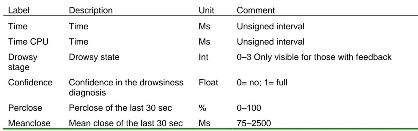
(28) Driver monitoring system (DMS) – Siemens VDO The DMS is a system developed by Siemens VDO. The system is video-based and focuses on providing support to drowsy or inattentive drivers. A compact camera and pulsed IR light is used, see Figure 10. The images are processed to extract information from the eye lid and blink patterns, eye gaze and face extraction. The system is fully automatic.. Figure 10 The DMS camera and IR source. The DMS provides three types of log files. The log file from the drowsiness detection is updated each 30 seconds and directly after each initialization, see Table 2. Table 2 The content of the DMS logfile in terms of label, description, Unit and specific comments. Label. Description. Unit. Comment. Time. Time. Ms. Unsigned interval. Time CPU. Time. Ms. Unsigned interval. Drowsy stage. Drowsy state. Int. 0–3 Only visible for those with feedback. Confidence. Confidence in the drowsiness diagnosis. Float. 0= no; 1= full. Perclose. Perclose of the last 30 sec. %. 0–100. Meanclose. Mean close of the last 30 sec. Ms. 75–2500. Drowsiness stage defined by the DMS is described at four levels, see Table 3.. 26. VTI notat 9A-2009.

(29) Table 3 The four different drowsiness stage used by the Simens system (DMS).. KSS The modified version (Reyner & Horne, 1998) of the Karolinska Sleepiness Scale (KSS) was used, see Table 4. KSS is a sleepiness scale that has been validated for driving situation (Åkerstedt & Gillberg, 1990). The participants rated their KSS levels in the laboratory before the drive started and after finishing the drive. Table 4 Karolinska Sleepiness Scale, as modified by Reyner and Horn (1998). Rate. Verbal descriptions. 1. extremely alert. 2. very alert. 3. alert. 4. fairly alert. 5. neither alert nor sleepy. 6. some signs of sleepiness. 7. Sleepy, but no effort to keep alert. 8. sleepy, some effort to keep alert. 9. very sleepy, great effort to keep alert, fighting sleep. VTI notat 9A-2009. 27.

(30) ORS The Observer Rating Scale (ORS) is an observation rating method which was developed for this experiment. It is based on observations of the driver and driver behaviour. The software was developed by Karolinska Instituet, and runs on a PC. With the ORS, the observer (test leader) sitting in the back seat classifies the driver behaviour and driving performance on the basis of a predefined scheme taking into account the driver’s: •. awareness. •. driving behaviour. •. blink behaviour. •. yawning. •. body position. •. body movements. The classification was done continuously. When specified criteria within the predefined scheme were observed, the test leader also changed the drivers ORS level. Every 5 minutes the test leader had to reconfirm the current ORS level, which was marked on the touch screen in grey. The ORS was recorded using a touch screen mounted in the car within easy reach of the observer (Figure 11). The ORS is coded in 5 levels (0–4): •. ORS 0 = no signs of sleepiness/normal wakefulness. •. ORS 1 = slight sleepiness, no micro sleep, fighting a little to stay awake, driving behaviour not affected. •. ORS 2 = some micro sleep, fighting sleepiness, slightly impaired driving. •. ORS 3 = micro sleep, stopped fighting sleepiness, severely impaired driving. •. ORS 4 = the driver is asleep, lane departures, incidents. Figure 11 The ORS touch screen as it was mounted in the instrumented vehicle. (Uppmärksamhet = Awareness, Körning = driving behaviour, Blink = blink, Gäsp = yawn, Kroppsposition = body position, Kroppsrörelse = body movements, Varning = Warning).. 28. VTI notat 9A-2009.

(31) The log file from the ORS software gives the time when an observation was made. The observations are presented with one column for each defined criterion. In the analysis, the selected ORS level was used as the true value until a new value was given, but observations of changes in the defined criteria were considered valid only at the moment (time frame) of reporting. There is interest in looking into the relationship between the ORS and other sleep indicators, for example parameters from the blink complex. There are a number of ways to analyse the relationship between the ORS and indicators from the blink complex. There are no natural links between the ORS and the registration of blinks. One way to compare the blink duration and the ORS is to compare the average ORS for each lap with the average blink duration. The definition of the interval for comparison is presented in Figure 12. We would like to emphasize that this is only one of several possible methods. Interval used for comparison. ORS 0. ORS 1. ORS 2. Seconds. Laps. Figure 12 Resolution of ORS and indicators from the blink complex. Figure 13 and Figure 14 present the blink duration and the ORS for each lap.. VTI notat 9A-2009. 29.

(32) Mean blink duration 130,00. 125,00. ms. 120,00. 115,00. 110,00. 105,00. 100,00 1.00. 3.00. 5.00. 7.00 Lap. 9.00. 11.00. 13.00. Figure 13 Mean blink duration distributed by lap (laps with pauses have been excluded). Error bars represent SE.. Mean ORS level. ORS mean. 0,80. 0,60. 0,40. 0,20 1.00. 3.00. 5.00. 7.00 Lap. 9.00. 11.00. 13.00. Figure 14 Mean ORS distributed by lap (laps with pauses have been excluded). Error bars represent SE. It is noticeable that both blink duration and ORS increased during the drive. The reason for the ORS drop at lap 8 is not known. It should be noted that laps with pauses have been excluded.. 30. VTI notat 9A-2009.

(33) A number of tests were performed in an attempt to validate ORS against different changes in, for example, blink duration and driving behaviour. The data were restructured into ORS bins (ORS0, ORS1, and ORS2) and those seen as repeated bins. An ANOVA was performed with a repeated measure design in order to see if there were any significant differences in driving or driver behaviour at different ORS levels. However there were only 10 participants in each group using a specific warning (early/late/feedback+late), and too few of them had driven during all ORS levels (at least 0, 1, and 2) for the ANOVA to produce reliable results. A more detailed analysis could be of interest, but will not be covered in this internal deliverable. Driving behaviour data Driving behaviour was recorded by the instrumented vehicle, at a sampling rate of 5 Hz; see Table 5. Table 5 Driving behaviour data recorded in the field trial. Label. Description. Unit. Comment. Dist. Distance travelled. m. Sampling starts at experiment start. Time. Time. sec. Time from start of sampling. Speed. Speed. km/h. latpos. Lateral position. m. LP. Reliability of latpos. Stwhan. Steering wheel angle. BR. Brake. Yes or no. BR. Blink right. Yes or no. BL. Blink left. Yes or no. RPM. Rev. counter. Yes or no deg. r/minute. Rotations per minute. 2. X-Acc. X-Acceleration. Ms. Y-Acc. Y-Acceleration. Ms2. Z-Acc. Z-Acceleration. Ms2. TR. Trigger. Starting point. VNR. Lap number. 1-max 30. Del. Section. 1–11. Hgr. Signed posted speed limit. km/h. 50- or 70-km/h. Data synchronisation With this setup, it is necessary to synchronise the data from the different systems. Synchronization between the EOG and the driving behaviour was achieved by sending a trigger signal from the computer which was recording driving behaviour to the Vitaport. The ORS and the DMS had synchronized clocks, and this synchronization was checked and adjusted during the experiment. As a fall back, the time lags in the different. VTI notat 9A-2009. 31.

(34) computers were saved continuously, and offline corrections were performed where necessary. Software has been developed by VTI in which driving behaviour data, ORS, and DMS log files are merged into one file. An example of the tool’s usage is shown in Figure 15. The software is written in CVI (C++). The sampling frequency of 5 Hz implies that at 70 km/h there will be 3.88 metres ((70/3.6)/5) and at 50 km/h there will be 2.78 metres between the data points. Data have been recalculated and reduced in order to have one value every 5 meters.. Figure 15 Example of the tool for data fusion and interpolation of missing data for lateral position. Data were recalculated from a time interval to a distance interval in order to make it easier to compare data between laps on the track and between test drivers. Analogue values were recalculated by identifying the distance to the nearest value before and after that point from the log file. The new value was calculated by linear interpolation between those two points (see Figure 16).. 32. VTI notat 9A-2009.

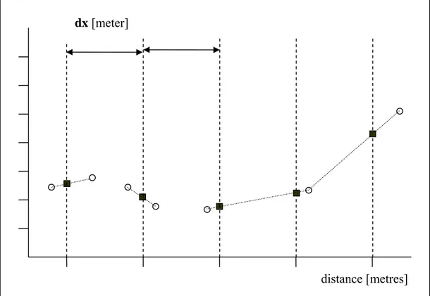
(35) dx [meter]. distance [metres] Figure 16 The recalculation of the time-based analogue values to distance where = measured values and = calculated values. For the digital values, the distance-based value was set to the largest value in the interval before that distance (Figure 17).. dx [meter]. distance [metres]. VTI notat 9A-2009. 33.

(36) Figure 17 The recalculation of the time-based digital values to distance where measured values and = calculated values. 3.5.6. =. Other recordings. All driving sessions were recorded on video, to allow recollection of what happened during the drive; for example, looking for signs of sleepiness in order to determine whether actions and lane departures were sleep related. 3.5.7. Trigger of the warning system. The warning system was triggered manually by the test leader; the decision to trigger the system was made with the help of the ORS level. The trigger was different depending on the condition. Condition. ORS level. HVMS level. ORS 1. HVMS 3. ORS 2. HVMS 5. Condition 3 – late warning. ORS 2. HVMS 3. Condition 4 – feedback and late warning. ORS 3. HVMS 5. Condition 1 – no warning Condition 2 – early warning. 3.5.8. Statistical analysis. The study used a between-participant design. ANOVA and non parametric one-way analysis of variance by ranks (Kruskal Wallis) were used for the analysis relating to countermeasures. ANOVA based on a mixed model (GLM) was used to analyse driving behaviour, with speed limit signs, warning conditions, and number of laps used as fixed factors. Participant was used as the random variable, grouped by condition. First-level interactions between condition and lap number and between speed limit sign and condition were included. All analyses were performed at a significant level of 5% (α=0.05). Data reduction Unfortunately there were some participants that due to different reasons needed to be excluded from the analysis. Table 6 presents the time, distance, and laps driven by each of the 40 participants.. 34. VTI notat 9A-2009.

(37) Table 6 Total observations per participant. Grey marked participants were excluded from further analysis because their driving time did not reach the limit of 1.2 hours (4322 sec.). Particip ant. Condition. time. 1. 2. 4447. 11073. 14.00. DMS out of order. 2. 2. 3596. 9459. 12.00. DMS out of order. 3. 2. 4934. 15005. 19.00. DMS out of order. 4. 1. 4322. 11903. 15.00. 5. 0. 7134. 19034. 24.00. 0. 3170. 8707. 11.00. Halted by test leader for safety reasons. 7. 1. 6708. 21488. 27.00. No video. 8. 2. 7265. 16668. 21.00. Fog. 9. 2. 6417. 19833. 25.00. 10. 3. 6769. 22268. 28.00. 11. 2. 7013. 22265. 28.00. 12. 0. 7081. 22246. 28.00. 13. 3. 7266. 17470. 22.00. 14. 1. 6885. 18308. 23.00. 15. 0. 6852. 22289. 28.00. 16. 1. 7360. 20673. 26.00. 17. 1. 7440. 20673. 26.00. 18. 3. 5324. 12709. 16.00. 19. 3. 7254. 18264. 23.00. 20. 0. 7141. 22253. 28.00. 21. 0. 6970. 18287. 23.00. 22. 0. 6973. 14173. 18.00. 23. 1. 7010. 18237. 23.00. DMS out of order. 24. 2. 6871. 20651. 26.00. DMS out of order, no vibrations. 25. 2. 7124. 21501. 27.00. 26. 3. 6992. 20661. 26.00. 27. 3. 7017. 22279. 28.00. 28. 1. 7118. 19859. 25.00. 29. 3. 7224. 22276. 28.00. 30. 0. 7032. 17431. 22.00. driven (seconds ). 6. VTI notat 9A-2009. distance driven (metres). laps. Comments. driven. No vibrations. No vibrations. DMS lights visible to participant. 35.

(38) Particip ant. Condition. time. 31. 3. 7250. 20632. 26.00. 32. 1. 7075. 15044. 19.00. 33. 0. 7242. 18272. 23.00. 34. 2. 7253. 19077. 24.00. 35. 0. 8118. 22234. 28.00. 36. 3. 7198. 21476. 27.00. 37. 1. 6989. 19816. 25.00. 38. 2. 6955. 19062. 24.00. 39. 1. 7266. 19078. 24.00. 40. 3. 7025. 20671. 26.00. driven (seconds ). laps. distance driven (metres). Comments. driven. DMS out of order. There were individual difference between driven time and driven distance (see Figure 18, depending on speed, number of stops, and the time each stop lasted. Time driven 2.50. Hour. 2.00 1.50 1.00 0.50. Subject. Figure 18 Time driven for each participant. To reduce problems with confounding, a selection of the data was made using the following criteria: − Speed above 20 km/h − Time driven between 0 and 4322 seconds (participants 2 and 6 excluded). The motivation for this was that two participants drove for less than 1 hour, and so to optimize the use of data the limit was set to 1.2 hours’ driving.. 36. VTI notat 9A-2009. 35. Total. 17. 16. 39. 8. 13. 19. 34. 31. 33. 29. 36. 5. 20. 25. 28. 12. 32. 30. 40. 27. 11. 23. 26. 37. 22. 21. 38. 14. 24. 15. 7. 10. 9. 3. 18. 1. 4. 2. 6. 0.00.

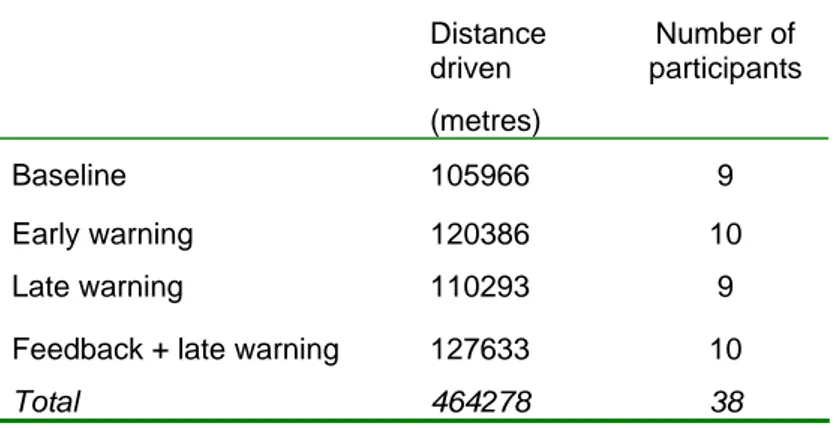
(39) Table 7 Observations – distance driven (selection of the first 1.2 hours driven). Distance driven. Number of participants. (metres) Baseline. 105966. 9. Early warning. 120386. 10. Late warning. 110293. 9. Feedback + late warning. 127633. 10. Total. 464278. 38. VTI notat 9A-2009. 37.

(40) 4. 4. Results. 4.1. Participants background. As mentioned in section 3.2, the study participants had an annual driven mileage between 5 000 and 50 000 kilometres, had no sleep-related illnesses, did not use drugs or medicines that results in decreased alertness, did not need glasses to drive, and were not pregnant. Upon arrival at the experimental site, participant filled out a questionnaire with some more details on their background with regard to driving experience, medication, and use of coffee and alcohol (Table 8). These data were mainly used to control for possible abnormalities in the data and to assist in the development of algorithms which are not included in this report. For the same purposes, participants also answered questions regarding possible sleep-related problems and sleep quality in general (Annex 11). Table 8 Participants’ backgrounds with regard to driving experience, medication, and use of coffee, alcohol etc. 20 male participants. 20 female participants. Age. 25–55 (mean 40). 25-55 (average 33). Annual vehicle mileage. 10.000–50.000 km (average 23.500 km). 10.000–45.000 km (average 18.500 km). Driving licence for. 2–37 years (average 22 years). 6–37 years (average 15 years). Weight. 65–100 kg (average 81 kg). 52–101 kg (average 71 kg). Height. 171–183 cm (average 178 cm). 155–182 cm (average 167 cm). Smokers. 4. 2. Snuff-takers. 5. 0. Users of stimulant beverages (e.g. coffee, Coke). 18, two of which drank more than 7 cups daily.. 18. Alcohol users. 20, one of which used it more than 4 days a week.. 19. Medicine users. 3; one used an anti-epileptic drug another was undergoing treatment for hypothyroidism, and the third used an anti-diabetic drug.. 4; one used an antidepressant and a beta-blocker, another used a beta-blocker, the third used birth control, and the fourth used painkillers.. ESS – Epworth Sleepiness Scale The Epworth Sleepiness Scale (ESS) (Johns, 1991) is a tool which takes into account how easy the participants find it to fall asleep in various situations (self-reported). The scale uses five steps from No chance of falling asleep to High chance of falling asleep, and the situations are: sitting and reading; watching television; sitting inactive in a public place (e.g. a theatre or a meeting); sitting as a passenger in a car for an hour without a break; lying down to rest in the afternoon when circumstances permit; sitting and talking to someone; sitting quietly after a lunch without alcohol; sitting in a car while stopped for a few minutes in traffic. The participant’s score is aggregated, and a total ESS score is calculated; the minimum total score is 0, which denotes not at all sleepy, and the maximum is 24, which denotes. 38. VTI notat 9A-2009.

(41) extremely sleepy. A score of 7–8 is considered to be normal. In our sample, six men and three women were less sleepy than normal, while six men and eleven women were sleepier than normal. A score of 14 is considered to be a critical limit; two men and one woman in our sample were above the critical limit. The distribution is shown in Figure 19.. 8 7 6 5 n 4 3 2 1 0 1. 2. 3. 4. 5. 6. 7. 8. 9. 10 11 12 13 14 15 16 17. ESS score. Figure 19 ESS scores of the participants. Restless Legs Syndrome The participants were asked whether they recognised the symptoms of restless legs syndrome: Do you have uncomfortable feelings or sensations in your legs (restless legs) combined with a desire to move your legs? Nine of the 40 participants answered yes; most of them stated that they felt these symptoms at least once a year but less than once a month. Sleep on the previous night For this experiment, it was important that the drivers were so sleepy that they would have trouble staying awake during the two hour test period, but it was also important that they were not so sleepy that it would be too unrealistic to start a 110 kilometre journey. Of the 40 drivers, one felt that he had slept enough and four that they had slept almost enough. There were also eight drivers who felt that they had slept far from enough (see Figure 20). Participants were also asked a number of more detailed questions regarding their sleep quality; these items are presented in Annex 3.. VTI notat 9A-2009. 39.

(42) Did you get enough sleep last night? 18 16 14 12 10 n 8 6 4 2 0 Yes, definitely. Yes, almost. Not quite enough. Not nearly enough. Far from enough. Figure 20 The test drivers’ views on whether they had got enough sleep during the night before the test. Fatigue/sleepiness-related traffic incidents/accidents Eleven of the participants (four men and seven women) had previous experience of incidents caused by fatigue/sleepiness, and a further three were uncertain about the question. Among the eleven with previous experience, two of the men claimed inattention, one committed a misjudgement, and the fourth had closed his eyes for a long time, but no incident resulted. Of the women, one claimed she nearly fell asleep, another fell asleep, a third nearly drove off the road, a fourth actually did drive off the road, and the remaining three described near accidents and periods of inattention. See Figure 21 and Annex 4 for more details.. Have you as a driver experienced incidents caused by fatigue/sleepiness? 30 25 20 n 15 10 5 0 Yes. No. Do not know. Figure 21 Drivers who had experienced incidents caused by fatigue/sleepiness.. 40. VTI notat 9A-2009.

(43) 4.2. Experiences of the test. One important purpose of this study was to examine the suitability of our method for evaluating drowsiness countermeasure systems. Aspects of interest are how the participants thought they performed during the test, whether they thought it was realistic, and how much effort they expended in order to drive as they did. The following presents the results of a post-test questionnaire, which is described in Annex 6. Regarding the question of how well they performed, most drivers felt that they had performed rather well; while a few felt that they had performed very well and a few very poorly, the majority lay in between (Figure 22). No differences were found between the four test conditions (Kruskal-Wallis one-way analysis of variance by ranks: χ2 (3) = 2.60; p=.457).. How well did you perform when driving? 6 No feedback or warning. 5 4. Early warning. n 3. Late warning. 2 Feedback and late warning. 1 0 Very well. Very poorly. Figure 22 Participants’ opinions on how well they performed when driving? In terms of how difficult it had been to stay awake when driving, most drivers thought that the effort required had been rather strenuous, though only a few stated that it was very strenuous (the top end of the scale), and a few thought it was not at all strenuous (Figure 23). This means that most of the drivers had to fight to stay awake during the test, to a certain degree. It is therefore reasonable to assume that they were in a state in which it would be beneficial from a safety point of view if they were persuaded to take a break, or to take some other action to counteract sleepiness while driving – that is, they were the target group for this experiment. However, no differences were found between the four experimental groups (Kruskal-Wallis one-way analysis of variance by ranks: χ2 (3) = 1.12; p=.772). The majority of the drivers felt it had required strenuous effort to stay awake while driving.. VTI notat 9A-2009. 41.

(44) How strenuous was it to stay awake when driving? 6. No feedback or warning. 5 Early warning. 4 n 3. Late warning. 2 Feedback and late warning. 1 0 Not at allstrenuous. Very strenuous. Figure 23 How strenuous an effort was needed to stay awake when driving? (Only the endpoints of the scale were defined.) The participants were all given a scenario to keep in mind when driving, in order to ensure that the test and their strategic choices were realistic, and as close to reality as possible (see section 3.4, Scenario). After the test, they were asked to rate how realistic they had found it; although most rated it at the top end of the scale, there were a few that did not find it realistic so there is still room for improvement (Figure 24). No differences were seen between the four comparison groups (Kruskal-Wallis one-way analysis of variance by ranks: χ2 (3) = 1.65; p=.649).. How realistic was driving compared to real driving? 7 6 5 4 n 3 2 1 0. No feedback or warning Early warning Late warning Feedback and late warning Not at all realistic. Very realistic. Figure 24 How realistic was the test compared to real driving? (Only the endpoints of the scale were defined.). 42. VTI notat 9A-2009.

(45) Sleepiness – KSS and ORS KSS The drivers reported their sleepiness on the KSS scale before and after the driving session; see Figure 25.. KSS before and after driving KSS_be KSS_af. 9,00 8,00 7,00. KSS. 6,00 5,00 4,00 3,00 2,00 1,00 .00. 1.00. 2.00. 3.00. Condition. Figure 25 Average KSS reported before and after the driving session. Condition: 0=baseline, 1=early warning; 2=late warning; 3=feedback + late warning. There were no significant differences in KSS levels between the test conditions (Kruskal Wallis before: χ2 (3) =1.72; p=.63; Kruskal Wallis after: χ2 (3) =1.27; p=.74). The driver reported higher sleepiness after the drive compare to before. The differences in KSS before driving and after driving were significant (Wilcoxon sign rank test Z=-5.3; p<0.01). ORS We would like to emphasize here that the primary interest of the study was the driver’s response (self reported or observed) to the SENSATION warning and its’ HMI. The analysis was therefore performed separately for different levels of driver sleepiness, here measured with the help of the ORS; see Figure 26.. VTI notat 9A-2009. 43.

(46) Distribution of observations at different ORS levels 100% Base line. 90%. Early warning. 80%. Late warning. 70%. Feedback + late warning. %. 60% 50% 40% 30% 20% 10% 0% ORS 0. ORS 1. ORS 2. ORS 3. Figure 26 Distribution of ORS levels on distance driven (1 value for every 5 metres). There was a significant difference between the distance driven for each condition within each ORS level (Condition: F(3,36) = 1.825; p=.160). Participants in group D (feedback + late warning) were in total sleepier during the experiment compared to participants in group A, B and D. In total, and regardless condition 32 participants reached ORS level 1, 17 participants reached ORS level 2, and 3 participants reached ORS level 3.. 4.3. Risk estimation/own capability. One of the problems related to driver sleepiness is that drivers do not always recognise how sleepy they are. In this study, only one person (male) reported falling asleep, while a further two were not sure. There were no differences between the conditions (group A–D). Even though only one person fell asleep, 17 others admitted that there had been a risk of their losing control of the vehicle because they were too sleepy, and another 5 were uncertain. Again, there were no differences between the four experimental conditions (Annex 6).. 44. VTI notat 9A-2009.

(47) 4.4. Received warnings. Drivers under test conditions 1, 2, and 3 could receive warnings. There were 26 warnings in total; see Table 9. Table 9 Number of received warnings based on 1.2 hours’ driving (Source=ORS). ORS 0 (n=38). ORS 1 (n=32). ORS 2 (n=17). ORS 3 (n=3). Baseline. 0. 0. 0. 0. 0. Early warning. 0. 9. 4. 0. 13. Late warning. 0. 0. 2. 0. 2. Feedback + late warning. 0. 0. 8. 3. 11. Total. 0. 9. 14. 3. 26. Total. There were no significant differences between conditions (Kruskal Wallis: χ2 (2) =4.39; p=.11). A more qualitative analysis regarding drivers’ actions when receiving a warning revealed additional information. If all data are used, including all warnings given based on the test leader’s observations, can be seen that 53 warnings were given in total. Table 10.presents the drivers’ responses to the warnings, in terms of stopping at the track/laboratory within 10 minutes of receiving the warning.. VTI notat 9A-2009. 45.

(48) Table 10 Warnings received, and participants’ responses (all warnings included). Condition. Early warning. Late warning. Feedback + late warning. Participant. Number of warnings. Stops at track/laboratory within 10 minutes. 7. 3. 0. 14. 1. 0. 16. 3. 3. 17. 5. 0. 23. 2. 0. 28. 3. 1. 32. 4. 0. 39. 1. 1. 3. 1. 0. 9. 1. 0. 11. 1. 1. 24. 2. 1. 34. 1. 1. 38. 2. 0. 10. 1. 0. 13. 6. 0. 18. 1. 1. 19. 3. 3. 26. 5. 5. 27. 2. 0. 29. 2. 0. 31. 2. 1. 36. 1. 0. 40. 2. 2. There were large individual differences between drivers’ responses, even within the conditions.. 46. VTI notat 9A-2009.

(49) 4.5. Recognising the sensation of sleepiness. Observed There were no significant differences between the conditions in the numbers of unconscious countermeasures (F(3,35) =0.392; p=.76); see Table 11. ORS level 3 was excluded from this analysis, since there were no observations for the early and late warning groups. Table 11 Drivers continuing driving – Observed body movements, changes in body position, or yawning. (Source: ORS). ORS 0. ORS 1. ORS 2. ORS 3. Baseline. 45. 68. 47. 16. 176. Early warning. 78. 112. 22. –. 212. Late warning. 56. 56. 18. –. 130. Feedback + late warning. 73. 97. 99. 19. 288. 252. 333. 186. 35. 806. Total. Condition. Total. When the drivers recognized that they were feeling sleepy, they began to take action in order to counteract sleepiness. Table 12 presents data on actions that could be performed without significantly interrupting the drive, for example opening the window, turning on the ventilation, or stopping for a short pause at the side of the track. The differences between conditions were not significant. Table 12 Drivers continuing driving – opening the window, turning on the fan, cold air, etc., or stopping at the side of the track to open the window/door. (Source: Test leader’s notes) Driving. Stopped at track. Condition. – opened window /fan/cold air. – open window/door. Baseline. 1. 3. Early warning. 1. 4. Late warning. 2. 5. Feedback + late warning. 0. 4. Self-reports The drivers were asked whether they did anything to stay awake during the experiment; a majority (24 persons) said they did, and another two drivers were uncertain. No differences could be found between the four conditions. Ten of the men did something to stay awake, with another two being uncertain, compared to 14 of the women; however, the difference was not statistically significant. Many different actions were taken to stay awake, such as lowering the temperature, opening the window, stopping. VTI notat 9A-2009. 47.

(50) for a while to stretch their legs, changing position, or stopping for a cup of coffee. See Annex 7 for full details.. 4.6. Stopping driving/taking a break. Only two countermeasures were seen as effective; stopping for a nap, or stopping for coffee. See Table 13. Table 13 Drivers that stopped at the side of the track for a nap, or stopped at the laboratory. (Source: Test leader’s notes.) Stopped at the side of the track. Condition. Stopped at laboratory. –sleep/closed eyes Baseline. 1. 3. Early warning. 0. 4. Late warning. 0. 1. Feedback + late warning. 3. 2. The differences between conditions were not significant. 4.6.1. User acceptance. There were no differences between the three experimental conditions that drove with a warning system activated for any of the findings below, hence they are not reported. For more detailed data on how the drivers responded, see Annex 8. Warning strategy Of the 30 drivers that drove with one of the warning/feedback systems, all except 3 stated that they received a warning. Of the 27 that received a warning, 20 stated that it did influence their driving, 3 said it did not, 2 did not know, and 2 did not answer the question. Most of the participants (23) reported that the warning made them more awake, while 4 thought it did not. They were, however, not so sure that it had helped them in any way; 4 drivers stated that it had not helped them and 6 drivers did not know. Still, 15 drivers thought it had helped them. 15 drivers thought the warning had come at the right time, 3 thought it was too late and 8 did not know. Of interest here is that none of the drivers thought that the warning came too early, and there were no differences between the drivers who received an early warning and those who received a late warning. See Table 14 for details.. 48. VTI notat 9A-2009.

No results found