Factor Investing on the
Swedish Stock Market
A Quantitative Study of a Model
Based on Quality and Value
Teodor Adolfsson, Henrik Domellöf
Department of Business Administration Civilekonomprogrammet Degree Project, 30 Credits, Spring 2018
Abstract
Investors and fund managers have, since the start of financial markets, always been on the lookout for new ways of beating the market. However, researchers of the Efficient Market Hypothesis have shown that markets are usually highly efficient, implying that there are few possibilities of earning returns that are higher than the market returns, on a risk adjusted basis. Prevailing theories, such as the Capital Asset Pricing Model, has shown that increased return must stem from taking on higher risk. Though, this model’s explanatory power has been challenged by numerous researchers who propose different factors, other than market risk, which could hold explanatory power when it comes to returns in the stock market. This area of research is called factor investing, and has shown that factors such as momentum, size, and value, all can lead to outperforming the market. This study examines how a model based on two common factors, quality and value, would have performed on the Swedish stock market. The study is based on five portfolios chosen by the quality and value factors, each one held for 5 years, examined over a 25-year time span and uses the capital asset pricing model as a tool to measure whether or not the selected factors outperform the market. The study has taken a quantitative approach to examining the research question, using a positivistic and objectivistic view.
The results of the study show evidence that the quality and value factors can lead to significant outperformance relative to the market index. Both total returns and risk adjusted returns were higher than the market index for some of the portfolios created using the quality and value factors. Furthermore, statistical evidence was found of that CAPM not fully explains all returns, and thus, that the returns are in part explained by the quality and value factors. The findings led to the conclusion that the quality and value factors does, in fact, hold explanatory power beyond that of CAPM. Purchasing quality companies at a reasonable price is shown to be a sound investment strategy, and that a portfolio created using the quality and value factors has good chances of outperforming the market index.
Keywords: Factor Investing, Quality Factor, Value Factor, ROE, Earnings Yield,
Efficient Market Hypothesis, Capital Asset Pricing Model, Swedish Stock Market
Table of Contents
List of Definitions ______________________________________________________ 1 1. Introduction ________________________________________________________ 3 1.1 Problem Background ______________________________________________ 3 1.1.1 Factor Investing _______________________________________________ 3 1.1.2 Common Factors ______________________________________________ 5 1.2 Problem Discussion _______________________________________________ 7 1.2.1 The Importance of Factor Investing _______________________________ 7 1.2.2 Choice of Factors ______________________________________________ 9 1.3 Purpose and Research Question _____________________________________ 10 1.4 Theoretical and Practical Contribution ________________________________ 10 1.5 Choice of Topic _________________________________________________ 11 1.6 Limitations _____________________________________________________ 11 2. Theoretical point of departure _________________________________________ 11 2.1 Theoretical Framework____________________________________________ 11 2.1.1 Efficient Market Hypothesis ____________________________________ 11 2.1.2 The Joint Hypothesis Problem ___________________________________ 12 2.1.3 Capital Asset Pricing Model ____________________________________ 13 2.1.4 Quality Factor _______________________________________________ 14 2.1.5 Value Factor ________________________________________________ 17 2.1.6 Factor Cyclicality ____________________________________________ 18 2.2 Previous Research _______________________________________________ 18 2.2.1 Fama and French _____________________________________________ 19 2.2.2 The Magic Formula ___________________________________________ 21 3. Method ___________________________________________________________ 21 3.1 Preconceptions __________________________________________________ 22 3.2 Literature Search_________________________________________________ 22 3.3 Scientific Approach ______________________________________________ 23 3.3.1 Ontological Assumptions ______________________________________ 23 3.3.2 Epistemological assumptions ___________________________________ 24 3.4 Research Approach and Methodological Choice ________________________ 24 3.5 Practical Method _________________________________________________ 25 3.5.1 Population __________________________________________________ 25 3.5.2 Factor Model and Portfolio Creation ______________________________ 25 3.5.3 Calculations and comparisons ___________________________________ 263.5.4 Problems ___________________________________________________ 26 3.5.5 Statistical Method ____________________________________________ 27 3.5.6 Method Discussion ___________________________________________ 28 4. Hypotheses ________________________________________________________ 30 5. Results ___________________________________________________________ 31 5.1 Hypotheses _____________________________________________________ 31 5.1.1 Portfolio 1 __________________________________________________ 31 5.1.2 Portfolio 2 __________________________________________________ 32 5.1.3 Portfolio 3 __________________________________________________ 33 5.1.4 Portfolio 4 __________________________________________________ 34 5.1.5 Portfolio 5 __________________________________________________ 35 5.1.6 Summary of Hypotheses _______________________________________ 36 5.2 Additional Data _________________________________________________ 36 5.2.2 Data from Regression Analysis __________________________________ 38 6. Analysis of Results __________________________________________________ 40 7. Discussion _________________________________________________________ 42 8. Conclusions _______________________________________________________ 45 8.1 Applicability of Results ___________________________________________ 45 8.2 Recommendations for Further Research ______________________________ 46 8.3 Ethical and Societal Considerations __________________________________ 46 9. Truth Criteria ______________________________________________________ 47 9.1 Reliability ______________________________________________________ 47 9.2 Validity ________________________________________________________ 48 Reference list ________________________________________________________ 49 Appendix ___________________________________________________________ 54 Portfolio 1 _______________________________________________________ 58 Portfolio 2 _______________________________________________________ 58 Portfolio 3 _______________________________________________________ 59 Portfolio 4 _______________________________________________________ 59 Portfolio 5 _______________________________________________________ 59
Appendix
Appendix 1. Selected stocks _____________________________________________ 54 Appendix 2. Monthly portfolio returns_____________________________________ 54 Appendix 3. Regression outputs __________________________________________ 58
List of Figures
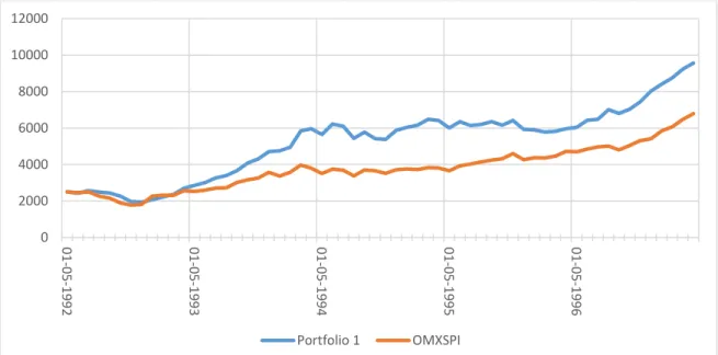
Figure 1. The performance of index and portfolio 1. __________________________ 31 Figure 2. The performance of index and portfolio 2. _________________________ 32 Figure 3. The performance of index and portfolio 3. __________________________ 33 Figure 4. The performance of index and portfolio 4. __________________________ 34 Figure 5. The performance of index and portfolio 5. __________________________ 35 Figure 6. The performance of OMXSPI 1992–2017 __________________________ 44
List of Tables
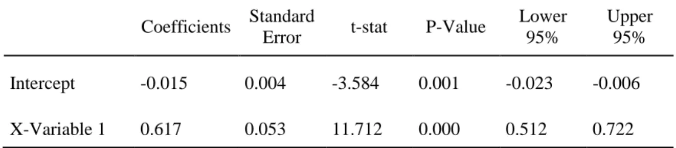
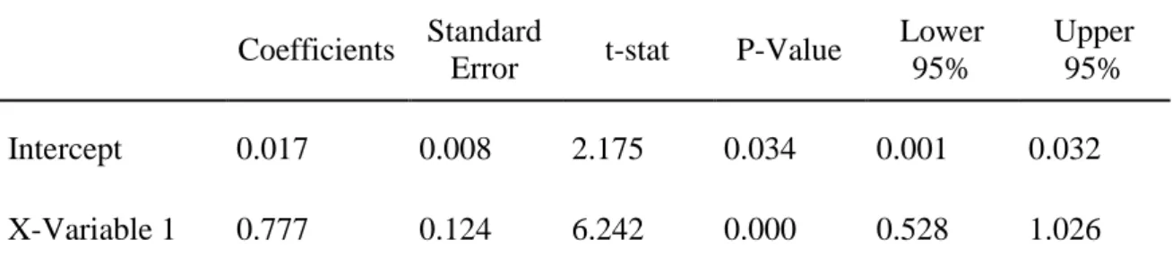
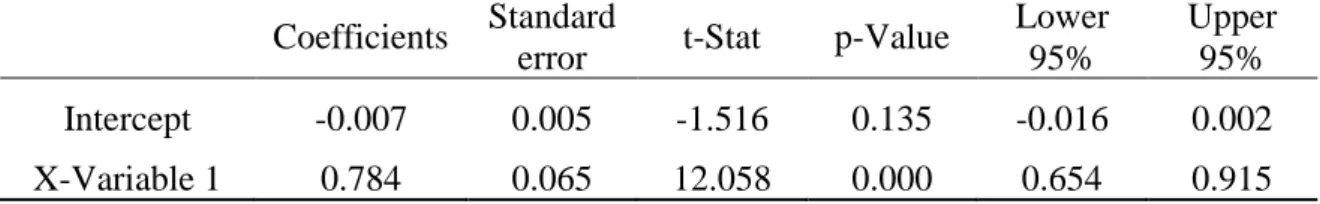
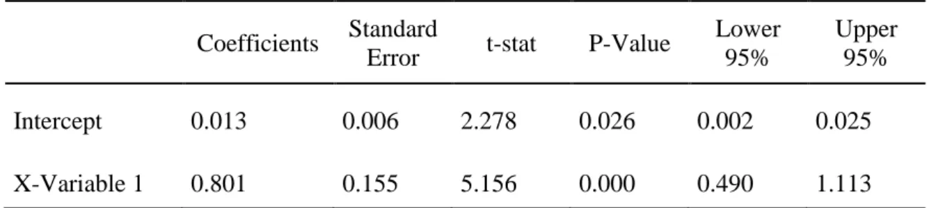
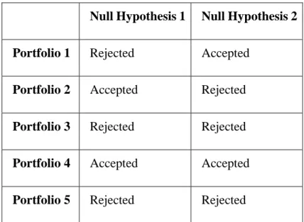
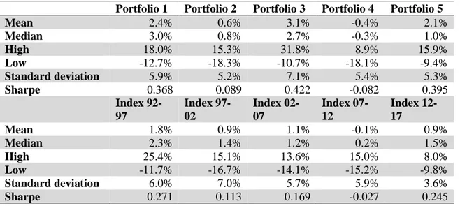
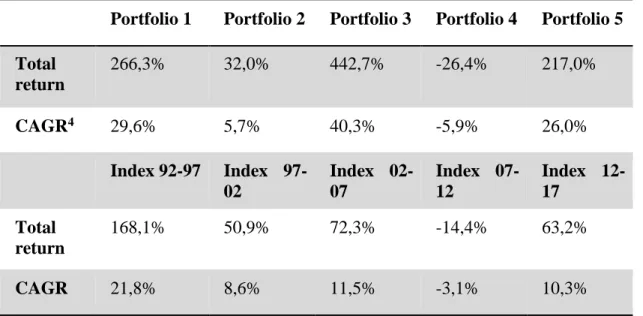
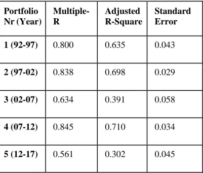
Table 1. Regression output, Rp1-Rf as dependent variable, OMXSPI-SDTB90D as explanatory variable ___________________________________________________ 31 Table 2. Regression output, Rp2-Rf as dependent variable, OMXSPI-SDTB90D as explanatory variable ___________________________________________________ 32 Table 3. Regression output, Rp3-Rf as dependent variable, OMXSPI-SDTB90D as explanatory variable ___________________________________________________ 33 Table 4. Regression output, Rp4-Rf as dependent variable, OMXSPI-SDTB90D as explanatory variable ___________________________________________________ 34 Table 5. Regression output, Rp5-Rf as dependent variable, OMXSPI-SDTB90D as explanatory variable ___________________________________________________ 35 Table 6. Summary of null-hypothesis outcomes _____________________________ 36 Table 7. Summary of portfolio returns and market index returns ________________ 37 Table 8. Summary of portfolio and index returns. ____________________________ 38 Table 9. Summary of Regression Statistics with portfolio excess return (Rp-Rf) as dependent variable and market excess return (Rm-Rf) as explanatory variable. _____ 39
1
List of Definitions
Factor Investing:
An investment strategy based on decomposing risk and return characteristics of one or a group of securities. There are two main types of factors within factor investing; macroeconomic factors and style factors. Macroeconomic factors aim at capturing risk and return characteristics inherent across asset classes whereas style factors aim at capturing risk and return characteristics inherent in specific asset classes. This study emphasises style factors, such as value, quality and momentum, among others.
CAGR:
Compounded Annual Growth Rate is the mean annual growth rate of the investment over the observed period.
pp:
Percentage point is the arithmetic difference of two percentages. For instance, a change from 4% to 5% implies a change of 1 percentage point (pp) whereas the percentage difference is 25%.
Portfolio Management:
The science and method used to steer the performance of the investment portfolio. Portfolio management aims at connecting the investment mix with predetermined objectives and includes aspects such as asset allocation, balancing risk and detecting strengths and weaknesses of the portfolio. Active Management:
The investment approach where human knowledge and choices determine the performance of the investment portfolio. Active management often integrate analytical research, forecasts and decisions based on practical expertise.
Passive Management:
An investment approach excluding the human element. Also referred to as “passive investing”, “passive strategy” and “indexing”. The method aims at replicating the movements and characteristics of an index.
Sharpe Ratio:
A measurement aiming to capture risk adjusted return. The higher the value of Sharpe ratio, the more attractive is the investment, considering the relationship between risk and return within the investment. Low risk and high return produce high Sharpe ratio whereas high risk and low return imply low Sharpe ratio.
Joint Hypothesis Problem:
In order to test whether the Efficient Market Hypothesis have flaws or not, risk and return has to be defined. To define risk and return, one has to use an asset pricing model. This creates what is called “the joint hypothesis
2 problem” which states that one of the theories cannot be tested without the other, that is, the Efficient Market Hypothesis cannot be tested without an asset pricing model (such as CAPM). The problem is that it is uncertain whether the results of flaws comes from the theory, Efficient Market Hypothesis, or the model chosen to define risk and return, CAPM.
Bear Market:
A period characterised by pessimism on the stock market, where securities prices fall over a period of time. The amount of securities sold exceeds the amount of securities bought. In short, bear market is a period of negative average growth on the stock market.
Bull Market:
A period characterised by optimism on the stock market, where securities prices rise over a period of time. There is a positive trend at stock prices rise over a given period, as the amount of securities bought exceeds the amount of securities sold. In short, bull market is a period of positive average growth on the stock market.
3
1. Introduction
The aim of this section is to present a background to factor investing, the relevance of this specific study and the importance of continuing to progress the research field of factor investing. This part will account for the history of factor investing and where the most common and researched factors derive from. Following, the importance of factor investing will be justified through declaring the potential benefit made possible by further researching and developing this area of research. Finally, the factors chosen to include in this study will be accounted for followed by the more concrete purpose, research question, theoretical contributions and limitations.
1.1 Problem Background 1.1.1 Factor Investing
Factor investing is the gathering name for the investment method of decomposing risk and return by factors that aims to explain the risk and return behaviour of an investment. It is a method for basing investments on scientifically proven factors that help explain a security’s risk and return, aiming to capitalize on those characteristics. Factor investing has attracted more focus as of recent years (Centineo and Centineo, 2017, p. 65), and is also known as smart beta (Centineo and Centineo, 2017, p. 68). Smart beta is mainly used as a marketing gimmick, with the purpose of pointing out that factors can enhance the returns1 on passive investing strategies, according to Centineo and Centineo (2017, p. 68). From here on, the authors will only refer to factor investing, but one can bear in mind that smart beta is simply an application of factor investing.
The systematic approach aims at capturing higher risk adjusted returns by strategically investing in different parts of the financial markets (Centineo and Centineo, 2017, p. 66) and has its roots in the well-known Capital Asset Pricing Model (Bender et al., 2013, p. 4), CAPM for short, developed by Sharpe (1964), Lintner (1965a, b), and Black (1972). The Capital Asset Pricing Model states that there is a linear relationship between expected return and market risk (Black, 1972, p. 455). More specifically, the development of CAPM in the late 1960’s came to provide a theoretical framework for pricing investments, displaying expected return as a function of the market risk sensitivity of the asset. It solely acknowledged and rewarded one common factor, the market risk measured as beta, for determining the expected return. It is important to understand that the CAPM lies as a foundation for factor investing (Centineo and Centineo, 2017, p.66). That is, discovering CAPM provided an explanation to why some investments require higher return than others. The CAPM states that higher market risk should be rewarded by higher returns, and this is precisely what factor investing is all about; finding factors, such as market risk in CAPM, that help explain risk and return characteristics of an asset. According to Centineo and Centineo (2017, p.66), factor investing emerged when traditional theories of efficient markets and asset pricing were challenged.
Improvements in technology allowed for better computational power and data. In turn, the field of research switched from being based on more normative theories, such as CAPM and the efficient market hypothesis, toward being observation driven and emphasizing empiricism (Centineo and Centineo, 2017, p.66). This allowed for tougher testing and discoveries of inconsistencies in prevailing theories. For instance, Haugen and Heins (1972; 1975) reviewed the relationship between risk and return and found that the
4 relationship was after all not fully linear, as the CAPM suggests. Investments regarded as having low risk showed a higher return than suggested by the linear risk and return relationship. Another example is Bhandari (1988), who found that high leverage ratios were connected to returns too high relative their beta. Discoveries like these led to the development of factor investing, which has, since then, become a well debated topic within research (Centineo and Centineo, 2017, p.68). To understand the roots of many of the factors used in factor investing, the efficient market hypothesis and its anomalies will be briefly explored, since it closely relates to the theory underpinning CAPM.
One of the main points of the efficient market hypothesis is that the price of an asset fully reflects all available information and that assets tend to be correctly priced at all time, as the price fully reflects the intrinsic value of the asset (Fama, 1970, p. 383), that is, if given equal access to information for all investors (Fama, 1970, 384-385). The empirical result showed extensive evidence in support of this theory, suggesting no possibility of earning abnormal returns (Fama, 1970, p.412). This entailed the assumption that the only possibility of earning higher returns is to take on higher risk (Fama, 1970, p.410), which suggests that there is no possibility of earning abnormal returns. The Efficient Market Hypothesis, and thus theory of abnormal return unattainability, was later reinforced by Jensen (1978, p.3) who said, “the Efficient Market Hypothesis is in essence an extension of the zero-profit competitive equilibrium condition from the certainty world of classical price theory to the dynamic behaviour of prices in speculative markets under conditions of uncertainty”.
Even though the Efficient Market Hypothesis has been widely tested and found to consistently depict different types of markets accurately, the study by Jensen (1978) showed on a few exceptions, or anomalies. Additional anomalies were later studied by Banz (1981), who found a phenomenon called the size-effect, Fama and French (1992), who found a pattern called book-to-market effect, and Ball and Brown (1968) who discovered a post earnings announcement drift. The existence of anomalies proves that markets are, in fact, not fully as efficient as they once were thought to be by Fama (1970). The anomalies discovered by Jensen (1978), Banz (1981), Fama and French (1992), and Ball and Brown (1968) somewhat prove that, even though markets generally are very efficient (Bodie et al., 2014, p. 380; Jensen 1978, p.1), there are indeed possibilities of achieving abnormal returns. Anomalies has since been a popular topic of research in the pursuit of achieving consistent abnormal returns, which is also why many factors in factor investing are based in these contradictions of the efficient market hypothesis.
Many anomalies have been studied and broken down into explanatory factors, and later included in different investing models. For example, the size effect, discovered by Banz (1981), the momentum effect, found by Jegadeesh and Titman (1993), and the value factor, explored by Fama and French (1992), and Basu (1975; 1977; 1983). In the following section, several factors commonly included in factor models are presented, all of which derive from one or another anomaly in the efficient market hypothesis.
5 1.1.2 Common Factors
A factor in general, is a characteristic for a group of securities, which holds explanatory power regarding the securities’ risk and return (Bender et al., 2013, p. 4). The most widely used factors are those that capture relevant stock characteristics, of which the most common and studied are momentum, value, size, quality, and low volatility (Centineo and Centineo, 2017, p. 69; Bender et al., 2013, p. 5).
The Momentum factor is defined as exposure to stocks that show the highest risk adjusted returns over the past 6 to 12 months (Centineo and Centineo, 2017, p. 69). This factor aims at capturing excess return from stocks with stronger past performance, and is usually captured by historical abnormal return, or relative returns last 3-, 6-, or 12 months (Bender et al., 2013, p. 5). The momentum factor was first developed by Jegadeesh and Titman (1993) who found that buying past winners and past selling losers gained significant abnormal return during their studied time period. Jegadeesh and Titman (1993, p. 89) studied the 1965 to the 1989 time period and found that the profitability of a relative strength strategy did not come from delayed stock price reactions to common factors but was consistent with delayed stock price reactions to firm-specific information. Jegadeesh and Titman (1993) suggests an interpretation of the results in line with the positive feedback trades studied by De Long et al. (1990). It suggests that investors who buy past winners and sell past losers make the price move away from their long-run values, and thus creating an overreaction in the prices (Jegadeesh and Titman, 1993, p. 90).
Before Jegadeesh and Titman, Ball (1978) discovered what is called the “post earnings announcement drift”, or PEAD-effect, as he studied the effects on what happened after a company made a public announcement, revealing consistent excess returns. He found that stocks tended to yield systematic excess returns on average in the period after an announcement (Ball, 1978, p. 103). The direction of the excess return was the same as the direction of the earnings deviations from the expectations (Ball, 1978, p. 103). Thus, if a firm deviated on the positive side, earning more than expected, the stock tended to earn positive excess return, and vice versa. Ball (1978, p. 103) also found some evidence that this excess return persisted over time. Ball (1978, p. 118) hypothesise that this effect was due to the earnings acting as a proxy, or due to a misspecification effect in the Sharpe-Lintner model used to measure returns. The findings of Piotroski (2000, p. 28) also point to the fact that the patterns of announcement period returns are inconsistent with the common notion of risk. He found that there was a relationship between the recent historical information, and both the future quarterly earnings announcements and the future performance (Piotroski, 2000, p. 38).
The Value factor is meant to capture excess returns from purchasing stocks that appear undervalued based on, for example, their earnings, book value, or cash flow (Centineo and Centineo, 2017, p. 69; Bender et al., 2013, p. 5). This is usually captured by, for example, book-to-market equity, earnings-to-price, sales, earnings, cash flow (Bender et al., 2013, p. 5). The most notable researchers on this particular factor are Fama and French (1992), Chan et al. (1991) and Basu (1975, 1977, 1983). Fama and French (1992) studied book-to-market equity among several other factors, and they found that book-to-market equity explained a lot of the return in stocks. This view is also taken on by Chan et al. (1991), who came to the conclusion that book-to-market equity worked well in explaining returns on the Japanese stock market. Chan et al. (1991) also studied how well earnings yield explained stock returns, and found that cheaper stocks outperformed more expensive stocks based on earnings yield. The more commonly known ratio, the
P/E-6 ratio, which is the inverse earnings yield, was studied by Basu (1975, 1977), who found that the informational value in the price-to-earnings ratio was not fully captured in the market. Basu (1977) also found that cheaper stocks, measured with price-to-earnings, outperformed more expensive stocks. Later, Basu (1983) studied earnings yield, and found that higher earnings yield was associated with higher risk adjusted returns than that of stocks with low earnings yield.
The Size factor is supposed to capture excess returns from exposure to stocks with a smaller market capitalization (Centineo and Centineo, 2017, p. 69; Bender et al., 2013, p. 5). The size effect refers to the outperformance of small stocks versus large stocks, usually measured as market equity/market value. Banz (1981) found that firms with large market values had smaller average returns than similar small firms (p. 8). Banz (1981, p. 11) therefore proposes that an additional factor, the market value of the firm's equity, is relevant for asset pricing. The study showed that the outperformance was not linear, and the magnitude of the effect varied over different ten-year subperiods (Banz, 1981, p. 16). The effect was largest for the smallest firms, and there does not seem to be any theoretical explanation to why it exists (Banz, 1981, p. 17). However, Banz (1978) showed that securities sought only by some investors have higher risk-adjusted returns, than those considered by all investors. This leads to Banz (1981, p. 17) conjecturing the informal model that the lack of information regarding small firms leads to lack of diversification and thus higher returns, because the smaller stocks appear undesirable. Since it is not clear why the size effect occurs, Banz (1981, p. 17) recommends interpreting it with caution, and urges investors to resist the temptation to use it, since it might be a proxy for something unknown. Van Dijk (2011) conducted a literature review where he seeks to examine the validity and existence of the size effect, following a discussion regarding if it has disappeared in more recent years. He sees two interesting developments in the literature regarding the size effect, the first being that the objections against the lack of theory behind the size effect has yielded several theoretical models explaining it, and secondly, that the empirical research shows that it has disappeared since the early 1980s (Van Dijk, 2011, p. 3263). The theoretical models where the size effect appears as an endogenous result of systematic risk (Van Dijk, 2011, p. 3263). Van Dijk (2011, p. 3272) concluded that it was too early to convict the size effect as dead, and points to the fact that the premiums for size in the US has been positive in the recent years. These findings are also an interesting anomaly in the EMH. Banz (1978; 1981), as well as Van Dijk (2011) have provided research regarding the outperformance of smaller companies versus larger ones. This is, perhaps, the most common anomaly in the EMH, and one that is very easy to point out. Van Dijk (2011) emphasised that there were a lot of discussion regarding whether the size effect still existed after Banz (1981) discovered it. According to Van Dijk (2011) it seems to be too early to claim that the size effect is gone, but the evidence might not be as strong as when Banz discovered it.
The quality factor refers to stocks with, for example, stable earnings and strong balance sheets, thus having high return on equity and low earnings variability and leverage (Centineo and Centineo, 2017, p. 69). Quality is commonly measured by return on equity, earnings stability, growth metrics, leverage and other balance sheet metrics, and softer variables such as the strength of the management (Bender et al., 2013, p. 5). This area has been researched by, for example, Piotroski (2000), who found that a portfolio based on book to market equity could be enhanced by applying fundamental analysis. This analysis should be aimed at finding and eliminating firms that might have poor future prospects, in other words, firms of low quality (Piotroski, 2000, p. 37). The quality factor was also
7 studied by Asness et al. (2013), who wanted to find out if investors were willing to pay a premium for higher quality companies. He created a factor, measuring the difference between high quality firms and lower quality firms, and found that investing in higher quality firms, while betting against lower quality firms would have been a good investment (Asness et al., 2013). Furthermore, Asness et al. (2013, p. 25-26) found that the quality premium tends to fluctuate, and that a low price for quality predicted higher return.
The final factor, low volatility, is defined as an optimized portfolio of stocks with lower volatility than the market index (Centineo and Centineo, 2017, p. 69). This is often captured by measuring the standard deviation on a one-, two-, or three-year horizon, measuring the beta, or by the downside standard deviation (Bender et al., 2013, p. 5). The low-volatility factor was discovered as Haugen and Heins (1975) examined the Capital Asset Pricing Model and found evidence against the relationship between risk and return (p. 872). The aim was to point out the shortcoming in the earlier empirical effort which supports the concept of a risk premium and measure the trade-off between risk and return. The empirical data Haugen and Heins (1975, p. 782) discovered did not support the notion that systematic- or non-systematic risk generates any kind of reward. Instead, Haugen and Heins (1975, p. 782) found that stock portfolios with lower monthly return variance had better return, in the long run, than similar portfolios with higher variance.
Conclusively, traditional theories and models such as the efficient market hypothesis and the CAPM have flaws. There are inconsistencies in the efficient market hypothesis and CAPM repeatedly fail to explain certain returns. This is where factor investing, which is somewhat an extension of CAPM, comes into place. Emerged from the inconsistencies and flaws of these theories, the strategy of factor investing aims to fill the gap between flaws and reality. Despite being subject of heavy criticism from numerous sources, CAPM and the efficient market hypothesis prevail as leading theories in business administration courses and practice. The following section will motivate why researching factor investing is, indeed, of great importance.
1.2 Problem Discussion
1.2.1 The Importance of Factor Investing
To this point in time, different theories have been developed in an attempt to understand why factors have historically earned a premium. One theory is that the returns by certain factors are a premium for taking on systematic risk, and another theory is that these returns derive from systematic errors, such as human behavioural factors and investor biases (Bender et al., 2013, p. 3). However, it is still unclear which theory depicts the reality best. Regardless of underlying theories and explanations to why specific factors have earned a premium, alternatives to factor investing are presented, since that explains why further research on factor investing is important.
In recent years, active management has come to compete with the increasing interest in passive management (Khorana et al., 1998). Jensen (1968) questioned the commonly held notion that actively managed funds outperform passively managed index funds. More specifically, Jensen (1968) questioned whether or not active management led to abnormal returns on investments. Studying mutual funds between 1945 - 1964, Jensen (1968) concluded that actively managed funds tended to underperform the average with approximately the same amount as the fees charged by the fund. This was later strengthened by the studies of Malkiel (2013, p.97) and Ennis (2005, p.45-46) which both,
8 also, showed on evidence that actively managed funds tended to underperform the benchmark net of fees. As actively managed funds tend to be both expensive and underperform the market average, index funds came to pose a cheap alternative with yet good return relative to actively managed funds. This led to a noticeable change in equity investing during the 1990s; index funds became very popular and a substantial increase of investments in index funds took place (Khorana et al., 1998). Index funds have since then been a popular choice of investment due to the low fees. The main points are that index funds are cheap but does not provide abnormal returns while actively managed funds are expensive and tend to underperform the benchmark but can, in some cases, result in abnormal returns.
Combining the advantages of active and passive management, factor based investing offers the possibility of abnormal returns while yet being cheap (Kahn and Lemmon, 2016, p.15). Traditionally, abnormal returns have been available through active management. The fact that specific factors may explain abnormal returns imply that the concept of abnormal returns can be broken down into (1) excess return explained by the actions and choices of the portfolio manager and (2) excess return explained by factors included in the portfolio. That is, theoretically, a degree of alpha return may be explained by certain factors included in an actively managed portfolio and not solely by the performance of the portfolio manager. The strategy of factor based investing aims to capture these factors that explain a part of the abnormal return. The advantages of factor investing for institutional investors could be significant. More specifically, getting a deep understanding of decomposed risk and return characteristics of groups of securities have most certainly great importance for actors active on the capital market. According to Bender et al. (2013, p.15), factor investing offers the best of two worlds; (1) the abnormal return of active management and (2) rule based and transparent characteristics of passive investing. Factor investing does not substitute active management but can partly contribute to a part of the value given by successful active management (Bender et al., 2013, p.15). As it offers a cheap alternative to active management and returns potentially above average the authors believe that factor investing is indeed important for developing further understanding of the explanation of returns as well as a competitive way of investing. In addition, the strategy offers two additional attributes valuable for investors; being rules based and transparent. Development of factor investing, through examining quality and value characteristics for example, is especially interesting for institutions, as it could give institutions good returns followed by reduced volatility yet giving access to specific assets (Centineo and Centineo, 2017, p.69-70). This would not only offer a better alternative than actively managed funds, but also passively managed index funds since it would ideally offer higher returns than average. It would not only facilitate the investment process for investors but also offer, if put in a model, a cost competitive investment strategy in favour of the investor.
As the fundamental importance of factor investing and the benefits one may obtain by not only considering one type of risk, but rather breaking it down into smaller explanatory components has been shown, the benefits of factor investing models will be shown. There is always a demand for better investment alternatives, especially those that are cheap and offers the possibility of earning high risk adjusted returns. It is no coincidence that the Sharpe ratio has become such a popular tool of measurement in the capital market. Institutions, private investors and non-private investors wish for good risk adjusted returns. Finding suitable and accurate models for factor investing is thus essential for contributing to a cheap, yet lucrative investment strategy. It is clear that factor models, if
9 succeeding to provide returns higher than the average, would provide a practical contribution to investors. If the model proposed succeeds with this, it will most definitely provide practical implications in the world of investments as well as a cost competitive alternative to prevailing alternatives. This motivates why further research in this field is needed. As there are numerous potential explanatory factors to investigate, the choice of factors founding this study will be discussed in the following section.
1.2.2 Choice of Factors
Now that the possible benefits of factor investing have been shown, the choice of factors for this study will be explained and motivated, which will lay the foundation for the research at hand. The choice is based on previous research underpinning the abnormal characteristics inherent in the quality and value factor, seen through the lens and statements of the Efficient Market Hypothesis
Value investing aims at purchasing companies that are priced at less than what they are intrinsically worth. Benjamin Graham paved the way for what is today called value investing (Buffett, 1984), and has become known as the father of value investing. Value investing is very closely linked to the value factor, but also incorporates several ideas captured in the quality factor. It is based on the theory that cheaper companies outperform more expensive ones, and the findings by the researchers who have studied the value factor tells us that there is evidence that such stocks can outperform on a risk adjusted basis. This is an important finding, since it shows that excess returns could be earned by selecting stocks that are cheaper. According to Lam (2002, p.178), cheapness could, however, be a proxy for additional risk, which is why the authors have chosen consider risk adjusted returns in the methodological part of this paper. Findings by Fama and French (1992) and Stattman (1980) and Rosenberg, et al. (1985, referenced in Fama and French, 1992) shows us that using book-to-market is an effective measure of value. Also, Basu (1975; 1977; 1983) and Fama and French’s (1992) three factor model tells us that it is viable to use the P/E ratio or earnings yield as an indicator of value.
Piotroski (2000) studied the relationship between quality and stock performance, concluding that there is a tendency of more profitable firms having higher returns. The choice of earnings yield and ROE as value and quality factors is further strengthened by Bender et al. (2013, p.5) who reviewed well-known systemic factors within the field of factor investing from academic research and by which measurements they were commonly captured. Since earnings yield was repeatedly encountered throughout the research of value factors as well as integrated in Fama and French three factor model, the authors consider it a suitable choice. Regarding the quality factor, Asness et al. (2013) found that quality firms tend to have high risk adjusted returns which makes the quality factor suitable for the model. Since ROE also was included among the most common measurements in the research on the quality factor (Bender et al., 2013, p.5), the authors find that to be a justified choice as well.
Thus, we have chosen the Value and Quality factors both because value is heavily supported in theory, and because some evidence shows that adding a measure of quality to a “value portfolio” can enhance the risk adjusted returns. The value factor is reasonably easy to capture, but the quality factor is a bit trickier. However, it is in line with the investing philosophy of famous investors such as Warren Buffett and Charlie Munger, and with our own personal investing philosophy. This philosophy can be explained as purchasing good companies at fair prices, or as Asness et al. (2013) puts it, Quality At
10 Reasonable Price (QARP). This is why we selected the combination of value and quality, even though the quality factor can be hard to capture.
1.3 Purpose and Research Question
The authors aim to investigate if the value factor and the quality factors combined give higher risk adjusted returns on the Nasdaq OMX Swedish Stock Exchange, and thereby returns higher than what the efficient market hypothesis and CAPM states that it should earn. In other words, does the value and quality factors contribute to consequently earning higher risk adjusted return than the market? The research question is as follows:
“Do portfolios including firms listed on the Swedish Nasdaq Stock Exchange selected based on quality and value factors have higher risk adjusted returns than the index when
assessed 5 years later?”
The authors will examine this research question by back testing a model which selects stocks based on the quality and value factors, and examine how it would have performed over 5-year periods for the last 25 years. As previously mentioned, the quality factor in the model will be measured as Return on Equity (ROE), and the value factor will be measured as Earnings Yield (Earnings-to-Price, E/P). The returns from this model will be measured against both the market index and capital asset pricing model in order to adequately answer whether or not differences in return is a product of taking on higher market risk or not. That being said, testing the factor model against the Efficient Market Hypothesis requires testing against an asset pricing model as well. The study will test the Efficient Market Hypothesis through CAPM, challenging them on what they can and cannot explain. In short, CAPM is the means by which the Efficient Market Hypothesis is tested in this study. A more thorough explanation of this requirement, choice and importance of CAPM is found in section 2.1.2.
1.4 Theoretical and Practical Contribution
With the aim to investigate whether value and quality factors give consequently abnormal returns, the practical contributions of this study are relevant to private and professional investors, investment managers and other practitioners in capital allocation. The authors aim to provide valuable evidence for or against using the quality and value factors in an investing model. In addition, they aim to add data to the factor investing field, regarding how investing based on quality and value factors combined have performed in the past. The authors also hope that their findings will give practical contributions to the investing field, by showing investors how factor investing have performed in the past, and thus inviting investors to the insight of how specific factors might perform in the future.
The theoretical contribution of this research is directed toward adding evidence for or against using the value and quality factors in a factor model. the authors wish to provide data on how these factors, when combined into a model would have performed historically on the Swedish market. Furthermore, they hope to contribute to further research and development of improved factor models. At this point, the authors know that factor investing can add significant benefits to investors and institutions due to offering the best of two worlds. That is, carrying the positive features of both active management and passive management.
11 1.5 Choice of Topic
The topic of investments has been of great interest since the authors began their education at Umeå University. In combination with the rise in index fund investments, the questioning of mutual- and hedge fund managers ability to achieve above index returns, and the rise of so called smart beta funds, they found the topic of factor investing to be highly interesting. Because, it might highlight characteristics of stocks that systematically outperform the market index as well as interesting insights both for the fund managers, stock pickers, and smart beta funds. Furthermore, it adds to the knowledge of what works in the stock markets and what does not. Since factor investing is an alternative approach of looking at the risk and return relationship and was never examined or presented in the finance courses during their education, the authors saw researching it as a compelling way of getting a profound understanding of the subject. It is also a topic where they believe more research is needed. For instance, it may provide better understanding of characteristics leading to stock outperformance, thereby helping improve portfolio management. Meaning, understanding the traits risk may help avoiding it, and, avoiding risk is undoubtedly of tremendous value to the financial market.
1.6 Limitations
This study is limited stocks listed on the Swedish stock market, defined as the large-, mid-, and small cap lists on the Nasdaq Stockholm Exchangemid-, and the stocks listed on First North. These lists were previously called A-listan (the A-list) and O-listan (the O-list). The authors have chosen to exclude stocks on over-the-counter exchanges, such as Alternativa Listan, Aktietorget, and Nordic MTF, because of the standardization of rules under which a company on a listed exchange must operate. Furthermore, the quality of the accounting is likely to be higher for companies on a listed exchange.
The holding periods of each portfolio is limited to 5 years each, and each of these periods will be examined. Hamilton (2005, p.6-7) depicts a business cycle as a fluctuation with the length of 3-5 years. Thus, the authors have chosen to hold the intended portfolios for 5 years each in order to capture a full business cycle. In addition, Bender et al. (2013, p.13) states that factor cyclical behaviour tends to stretch over 2- to 3-year period, with only rare findings of periods stretching over 5 years, which strengthens the choice of a 5-year timeframe for the holding periods.
2. Theoretical point of departure
2.1 Theoretical Framework
This section will present the theories and previous empirical studies related to factor investing, and in turn, fundamental for this study. It starts with the Efficient Market Hypothesis, and moves on to the Capital Asset Pricing Model, after which the Quality factor and the Value factors are introduced further, which are the factors this study intends to investigate. Furthermore, this section includes an explanation of factor cyclicality, and presents relevant previous research into factor investing models.
2.1.1 Efficient Market Hypothesis
In a market, where all participants are given equal access to information, the efficient market hypothesis suggests that the price of an asset fully reflects all available information (Fama, 1970, p.383). Fama (1970) presents three forms of market efficiency; weak form, semi-strong form and strong form. The weak form is based on the research
12 around the random walk theory of asset prices, and regards information carried by historical prices. The semi-strong form regards the price adjustment to reflect new publicly available information, such as earnings announcements for example, and the strong form suggests that all information, private or public, is accounted for in the asset’s price (Fama, 1970, p.383). There are, however, numerous inconsistencies in the efficient market hypothesis (Jensen, 1978; Banz, 1981; Fama and French, 1992; Ball and Brown, 1968; Jegadeesh and Titman, 1993; Basu, 1975; 1977; 1983). These inconsistencies are called anomalies and points to characteristics giving systematically higher returns than suggested by the efficient market hypothesis (Jensen, 1978, p.4-8). In order to determine if returns are, in fact, abnormal one must consult an asset pricing model, where the Capital Asset Pricing Model is the most commonly used.
2.1.2 The Joint Hypothesis Problem
The following section gives an explanation to the choice and inclusion of CAPM in the practical method as well as the importance of testing the Efficient Market Hypothesis through an asset pricing model. It will answer the question to why CAPM plays such an important role in the practical method as well as in this study.
For a strategy to violate the Efficient Market Hypothesis, it is not simply sufficient that it consequently earns higher returns than the market. Higher risk should, in theory, be rewarded with higher returns. Earning consequently higher returns than the market could therefore be explained by taking on higher risk. A portfolio taking on greater risk than the market may be thus also be rewarded with higher returns. This suggests that in order to examine whether or not a strategy violates the Efficient Market Hypothesis or not, one has to take into account the riskiness of the strategy. This may be accomplished by testing the returns against the Efficient Market Hypothesis through an asset pricing model, such as CAPM for example, as it specifies how much reward an asset should earn due to its inherent risk. However, there are different asset pricing models, such as CAPM, Arbitrage Pricing Theory, and Fama-French Three Factor Model. As the models differ from each other, the specifications of risk and return differ between them as well. This poses a big problem for testing the Efficient Market Hypothesis, since the choice of asset pricing model affects the outcome due to their different specification of risk and return. One will, in other words, be dependent on the choice of asset pricing model. It becomes a joint hypothesis problem, as testing the Efficient Market Hypothesis requires testing a model as well. This implies that a miss-specified asset pricing model may lead to the wrong conclusion when testing the Efficient Market Hypothesis. Thus, two things can go wrong; one or two of the hypotheses is false or the joint hypothesis is false, and you cannot distinguish which one it is. (Fama, 1992; Jensen, 1978)
As explained above, in order to examine whether the quality and value factor violates the Efficient Market Hypothesis, firstly defining risk and return through selecting an appropriate asset pricing model is required, and, secondly, a joint hypothesis test has to be executed. In this study, CAPM has been selected as the asset pricing model founding the test of the Efficient Market Hypothesis. In short, CAPM is the means by which we can test the Efficient Market Hypothesis. The choice of CAPM is based on it being the model used to greatest extent in previous research of factor investing as well as it being greatly recognized within both the practical and theoretical field of economy.
13 2.1.3 Capital Asset Pricing Model
The Capital Asset Pricing Model was developed by Treynor (1961), Sharpe (1964), Lintner (1965) and Moussin (1966). The model proposed that the return of an investment was to be relative to the market risk associated with that same investment. It showed on a linear relationship between the two factors (1) expected return and (2) market risk, where an investment with high market sensitivity would require a high expected return, and vice versa. Black (1972) further explored the model, by constraining the hypothetical investors access to a risk-free asset. First by removing it entirely, then by only allowing long positions in the risk-free asset (Black, 1972, p. 455). Black (1972, p. 455) also found that the expected return on a risky asset must be a linear function of its beta. If the borrowing is restricted, the slope on the expected return is lower than in the case where the investor has access to borrowing (Black, 1972, p. 455). CAPM as a formula is usually written as: E(Ri) = Rf + Bi[E(Rm) - Rf], where E(R) is the expected return, B is the beta, E(Rm) is the expected market return, and Rf is the return on a risk-free asset. The Beta is calculated as the covariance of the market return and the return on the risky asset, divided by the variance in the market return. CAPM uses the assumptions (1) that all investors hold the same opinions about the values for all assets, (2) the probability distribution of the possible returns are joint normal, (3) investors are wealth maximizing and risk averse, and (4) an investor can take both long and short positions in any asset, meaning that the investor can both borrow and lend at the risk-free rate (Black, 1972, p. 444). This is known as the Sharpe-Lintner-Black model. A study by Fama and French (2004, p.25) clarifies that the CAPM became very popular ever since, and has for over four decades been widely used in both practice and for educational purpose; the model’s simplistic properties, yet powerful prediction power of the risk and return relationship, has made it a very popular tool for quite some time. This, despite criticism from, among others, Roll (1977), who proposed the Market Proxy Problem, which criticizes the capital asset pricing model due to the difficulties of defining the essential component market portfolio.
Challenging the CAPM, Fama and French (1992), Statman (1980), Rosenberg, et al. (1985, referenced in Fama and French, 1992) and Chan et al. (1991) sought out to investigate risk and return relationships, studying the relationship between value and stock performance, concluding that there was, indeed, a tendency that cheaper stocks gave higher risk adjusted returns. Further research was done by Piotroski (2000), who studied the relationship between quality and stock performance, finding that more profitable firms tend to have higher returns. More specifically, evidence showed that among high Book-to-Market firms, the healthiest firms appeared to generate the strongest returns (Piotroski, 2000, p.28). This led to different models being developed in order to capitalize on such anomalies. There is evidently a theme of contradictions to the CAPM model, where Beta repeatedly throughout studies lack to explain certain returns (Fama and French, 2004, p.35-36).
Further critique to CAPM was presented by Ross (1976) who proposed the Arbitrage Pricing Theory. The Arbitrage Pricing Theory was an asset pricing model, just as CAPM, but estimated the return of a single asset through a linear combination of many independent macroeconomic variables (Ross, 1976, p. 341-343). The development of the Arbitrage Pricing Theory came to be a continuation of the theoretical foundation for factor investing as it allowed for many different sources of systematic risk in contrast to the CAPM, which only allowed one type of systematic risk.
14 2.1.4 Quality Factor
This section will present theory and empirical evidence regarding the quality factor. This will serve as a foundation for the choice of including the quality factor in this study, and will show that it does in fact have power to improve the performance of a value factor portfolio, and thus outperform the market index. The quality factor is somewhat difficult to define, but common definitions include earnings stability, dividend payouts, investment levels, profitability, cash flow, level of accruals, etc.
Piotroski (2000) finds that the distribution of the return of a broad book-to-market portfolio can be shifted by applying a simple accounting based fundamental analysis. Piotroski (2000, p. 28) found that among high Book-to-Market firms, the healthiest firms appeared to generate the strongest returns. Piotroski (2000, p. 37) therefore suggests that a generic Book-to-Market portfolio can be improved by using relevant historical information in order to eliminate firms with weak future prospects. Furthermore, Piotroski (2000, p. 37) found that the benefit of financial statement analysis of the high Book-to-market firms was concentrated to small and medium sized firms, with low share turnover, and no analysts following. Piotroski (200, p. 38) also found that there is a relationship between the historical information, and to both the subsequent quarterly earnings announcements and the future performance. This implies that using fundamental analysis in order to assess firms based on quality, can improve the performance of the portfolio.
In contrast to Piotroski (2000), this is also explored by Mohanram (2005), who instead studied the effect of financial statement analysis on low book-to-market portfolios, known as portfolios of growth stocks. Mohanram (2005) points to the empirical phenomenon that low book-to-market portfolios tend to underperform relative to the market, which is also shown in the previous section, but also points to the fact that the variation in stock return is considerable. The author is thus going to apply financial statement analysis in order to try and separate the winners from the losers in a low book-to-market portfolio (Mohanram, 2005, p. 137). Low book-book-to-market firms are defined as ratios below the 20th percentile for the entire market, and Mohanram (2005) uses three categories of signals when doing the financial statement analysis (Mohanram, 2005, p. 138). These groups of signals are defined as; Category 1: Signals based on Earnings and Cash Flow Profitability, Category 2: Signals Related to Naive Extrapolation, and Category 3: Signals Related to Accounting Conservatism (Mohanram, 2005, p. 138). Category one includes measures such as Return on Assets using Net Income before extraordinary items divided by total assets (Mohanram, 2005, p. 138). It also includes a binary measure, which checks if the cash flow return on assets exceed the the median of all low book-to-market firms in the same industry (Mohanram, 2005, p. 139). The final measure in the first category concerns whether or not the cash flow exceeds the net income of the firm (Mohanram, 2005, p. 139). In the second category Mohanram (2005, pp. 139-140) uses a measure which concerns the variability of earnings relatively to all low book-to-market firms in the same industry, and a measure the variability in sales growth also relatively to all low book-to-market firms in the same industry. The final category includes three measures, which checks if a firm's research and development, capital expenditure, and its advertising spending, are higher than other low book-to-market firms in the same industry (Mohanram, 2005, p. 140). These measures are aggregated into what Mohanram (2005) calls GSCORE. Mohanram (2005) employs a strategy that buys firms with a high GSCORE and sells firms with low GSCORE. The findings indicate that this strategy is able to differentiate the winning stocks from the
15 losing ones, which is shown by the fact that high GSCORE firms earned substantially higher returns than the los GSCORE firms (Mohanram, 2005, p. 166). However, Mohanram (2005, p. 166) notes that much of this performance comes from the gains on the short positions in the low GSCORE firms, and thus the strengths of this strategy lies in its ability to find the stocks to avoid. Furthermore, when controlling for factors such as book-to-market, accruals, momentum, etc, GSCORE is positively correlated with future returns over a long time period (Mohanram, 2005, p. 166). Mohanram (2005, p. 167) argue that these results must be because of the misinterpretation by investors regarding the financial information given by firms, which is contrasted to the findings by Piotroski (2000) which point to ignorance of certain information. These findings by Mohanram (2005) show, like the findings by Piotroski (2000), that fundamental analysis of the firm's financial information, in order to discover its inherent quality, can lead to excess return and improves a portfolio created using book-to-market.
Fama and French (2006) explored the book-to-market equity, together with the expected profitability, and the level of expected investments. Fama and French (2006, p. 495) create a proxy for profitability on investments, using cross-section regressions. These fitted values from the regressions are then used in the cross-section return regression, which tests the effect of profitability and investments on the stock return (Fama and French, 2006, p. 495). These tests exclude financial companies, and is mostly during 1963 - 2003 (Fama and French, 2006, p. 496). For example, Fama and French (2006) found that firms with high dividends, high levels of accruals, and high book-to-market ratio, grew their assets more slowly. On the other hand, smaller firms, firms with lower dividends, low book-to-market, and low accruals, grew faster (Fama and French, 2006, p. 495). Regarding profitability, they found that profitability is both persistent and mean reverting (Fama and French, 2006, p. 501). Furthermore, they found that high book-to-market firms were less profitable, and non-dividend paying firms are also less profitable (Fama and French, 2006, p. 501). In order to test how these factors impact the expected return, Fama and French employ three steps: (1) using simple cross-section regressions to examine how they add to the explanation of stock returns provided by size and book-to-market equity, (2) using more complicated proxies gathered from fitted values from the regressions, and (3) using portfolios to examine if the profitability and investment effects persist (Fama and French, 2006, pp. 502-503). Fama and French (2006, p. 514) find that high book-to-market equity had higher expected returns when controlling for expected profitability and investments. When given the book-to-market and the expected profitability, higher investments correlated with lower return (Fama and French, 2006, p. 514. Fama and French (2006, p. 514) find that these results are in line with the the existing evidence, both that book-to-market equity has good descriptive power, and that more profitable firms have higher expected returns, while more investments or higher level of accruals are associated with lower returns. Thus, this shows evidence that examining the firm's quality, based on profitability, or level of investments, can improve the explanatory power of the book-to-market equity measure.
Asness et al. (2013) examined if investors were willing to pay more for quality. They claim that high-quality stocks have earned high risk-adjusted returns, and low-quality stocks have had negative risk-adjusted returns (Asness, et al., 2013, p. 2). They found that a Quality-minus-Junk factor (QML) going long high-quality stocks, and shorting low-quality stocks earned high risk adjusted returns (Asness, et al., 2013, p. 25). Asness et al. (2013, p. 3) uses Gordon's growth model to express the price-to-book as P/B = (Profitability * pay-out ratio) / (Required return - growth). This leads them to identify
16 four factors of quality, and thus factors an investor would want to pay an increased price for (Asness, et al., 2013, p. 2-4). The four parts of the quality assessment are profitability, growth, safety, and pay-out ratio (Asness, et al., 2013, p. 3-4). Profitability is defined as profit per unit of book value, and all else equal, a more profitable firm deserves a higher stock price (Asness, et al., 2013, p. 3). Asness et al. (2013, p. 3) also suggest that an investor would want to pay more for a firm that is growing its profits, and that an investor should pay a higher price for a safer stock. Safety is defined by Asness et al. (2013, p. 3) as a stock with lower volatility, and thus lower beta, and a lower required rate of return. Pay-out ratio is defined by Asness et al. (2013, p. 4) as the fraction of profits that gets paid out to shareholders. This can be seen as a measure of shareholder friendliness, and is decided by the managers (Asness, et al., 2013, p. 4). Asness et al. (2013, p. 4) point out that if a higher pay-out ratio is achieved at the cost of growth or lower future profitability, an investor should not pay more for it, but if all else is equal, higher pay-out should be positive. According to Asness et al. (2013, p. 4) the companies that are profitable, growing, stable, and has high pay-out ratio, continue to show the same characteristics on average over the next five or ten years. Furthermore, Asness et al. (2013, p. 5) found that the Quality minus Junk factor performed well, and during market downturns it did not crash, but instead showed mild positive convexity, therefore benefitting from investors moving toward quality in market turmoil. Asness et al. (2013, p. 6) also combines the Quality minus Junk idea with the High Minus Low (HML) idea from Fama and French (1992), into what Asness et al. call Quality at reasonable price (QARP). While the QML buys and sells based on quality measures, irrespective of price, HML does the reverse, it buys solely on price, and ignores quality (Asness et al., 2013, p. 6). Combining the two into QARP improves the value investing, which is consistent with what Graham and Dodd (1934, referenced in Asness et al., 2013, p. 6) writes, and with what Piotroski (2000) found. Finally, Asness et al. (2013, p. 25-26) found that the price investors are willing to pay for quality vary over time, and that low price of quality was a predictor of high future return. These findings implicate that higher quality firms outperform lower quality firms, and thus gives reason to believe that selecting stocks based on their quality can lead to abnormal returns.
Regarding the quality of a firm's accounting, Perotti and Wagenhofer (2014) examined how common measures of earnings quality improved the decision quality of a company’s reporting for investors. They hypothesized that firms with higher earnings quality will be less mispriced than firms with lower earnings quality (Perotti & Wagenhofer, 2014, p. 545). The mispricing was measured as the difference if the mean absolute excess return of portfolios of high values of the quality measures, versus portfolios of low measures in quality of earnings (Perotti & Wagenhofer, 2014, p. 545). Perotti and Wagenhofer (2014, p. 567) constructed the portfolios based on eight different measures of earnings quality, namely persistence, predictability, abnormal accruals, accrual quality, earnings response coefficient, and value relevance. They found that the earnings smoothness, measured as the persistence and as predictability, had a positive relationship with absolute excess return (Perotti and Wagenhofer, 2014, p. 567). Furthermore, they found that accruals measures were the most useful earnings quality measures (Perotti and Wagenhofer, 2014, p. 567). This is somewhat related to a study whether or not stock prices reflect the information carried in accrual and cash flow parts of the firm's earnings, Sloan (1996) found that investors tend to fixate on earnings, thus not making the stock price reflect the values generated in accruals or cash flows. Sloan (1996, p. 290) found that the earnings related to accruals showed less persistence than earnings related to cash flow. Thus, Sloan (1996, p. 290) concludes that firms with high levels of accruals have lower future
17 abnormal stock returns, and those with less accruals have higher levels of abnormal return. This abnormal return is concentrated around future earnings announcements (Sloan, 1996, p. 290). Sloan (1996, p. 306) found that and investor could earn abnormal returns by abusing the fact that stocks were not priced according to the information carried in the accrual and cash flow parts of earnings. Even though not directly linked to this study, this shows evidence that assessing companies based on their quality can pay off.
Even though there are several definitions on what makes a company higher quality, for example better earnings stability, quality of accounting, and level of profitability, these studies show that it might be possible to achieve abnormal returns by thoroughly researching a company’s financials, and that there might be abnormal returns from finding higher quality companies to invest in.
2.1.5 Value Factor
The theory and empirical evidence presented in this section will serve as a foundation for the choice of the value factor in this study. The theories and empirical evidence shows that the value factor can outperform the market index on a risk adjusted basis, and gives us reason to believe it is worthwhile to include it in this model. The value factor refers to the finding that stocks that are cheaper have outperformed stocks that are more expensive. Cheapness is usually measured by book-to-market equity (Book value of equity/Market value of equity), earnings yield (Earnings/Price), Price-to-earnings (Price/earnings), or in some cases as dividend yield.
According to Fama and French (1992, p. 450) size, and book-to-market equity captures the cross-sectional variation in stock returns associated with size, earnings yield, book-to-market equity, and leverage, for the 1963 to 1990 period. Furthermore, Stattman (1980) and Rosenberg, et al. (1985, referenced in Fama and French, 1992) finds a positive relationship between average return and Book-to-Market equity on the US market. These findings showed evidence of outperformance by cheap stocks over more expensive stocks.
Chan et al. (1991) also studied the effect of book-to-market equity, and found that it is a powerful variable to explain returns on the Japanese market. In their study, Chan et al. (1991, p. 1761) studied other value measures as well, such as cash flow yield and earnings yield. However, they found that book to market equity and cash flow yield had the strongest impact on expected returns on the Japanese stock market (Chan et al., 1991, p. 1761). Regarding earnings yield, Chan et al. (1991, p. 1761) found that a strategy holding high E/P stocks outperformed a strategy that held low E/P stocks. Basu (1977) explored the relationship between the P/E ratio and the investment performance of common stocks. He found that during the time period April 1957 to March 1971 portfolios with low price-earnings ratios earned higher absolute and higher risk adjusted returns than high P/E portfolios on average (Basu, 1977, p. 680). Basu (1983) also studied the relationship between earnings yield (E/P ratio), market value, and return for common stocks on the New York Stock Exchange. Basu (1983, p. 150) found that during 1963 to 1980 the return on stocks listed on the NYSE was related to the firm size and the stocks earnings yield. The stocks of high earnings yield firms earned higher risk adjusted returns on average, than the firms with low earnings yield (Basu, 1983, p. 150). Furthermore, this earnings yield effect seemed to vary inversely with firm size, meaning that it was weaker for larger than average firms, and stronger for smaller than average firms (Basu, 1983, p. 150). Basu (1983, p. 151) concludes that the earnings yield effect is more complicated than