Exchange rate volatility : How the Swedish export is influenced

J

I

B

S

E x c h a n g e r a t e v o la t ili t y

How the Swedish export is influenced

Master Thesis within ECONOMICS Author: Mikaela Backman

Tutor: Scott Hacker, Associate Professor James Y. Dzansi, Ph.D Candidate Jönköping June 2006

Master Thesis in Economics

Title:

Author

Tutors:

James Y. Dzansi, Ph.D Candidate

Date:

Keywords:

Abstract

The purpose of this thesis is to examine whether the exchange rate volatility has an impact on Swedish exports. This relationship has been tested in several studies but no consistent result has been found. It is therefore an interesting subject to investigate further and it has not been thoroughly tested for Sweden using aggregated data. Since the exchange rate vola-tility may have an effect on exports, and therefore on the whole economy, the effect can support a certain exchange rate regime. All the data used in this thesis is based on the ag-gregated data for Sweden and the Euro zone between the years 1993 and 2006. The method chosen is a statistical analysis using regressions. Three variables other than ex-change rate volatility were included when conducting the regressions explaining Swedish exports and these are: the real effective exchange rate index, the industrial production in Sweden (“push” factor) and the import from the Euro Zone (“pull” factor). The overall conclusion found was that the industrial production in Sweden, the real effective exchange rate index, the time and lagged values of the export influence the export. There was no evi-dence found that the exchange rate volatility influences the exports for Sweden.

Magisteruppsats inom Nationalekonomi

Titel:

Författare:

Handledare:

James Y. Dzansi, Doktorand

Datum:

Nyckelord:

Sammanfattning

Syftet med denna uppsats är att undersöka om förändringar i växelkursen påverkar den svenska exporten. Sambandet har testats i ett flertal studier men inget konsekvent samband har hittats. Detta gör det till ett intressant ämne att vidareutveckla. De flesta undersökning-ar som hundersökning-ar gjorts hundersökning-ar ej använt den aggregerade nivån i Sverige. Eftersom fluktuationen i en växelkurs kan påverkar ett lands export, och därför hela ekonomin, kan effekten av denna påverkan stödja en viss växelkursregim. Datan som används utgörs av åren 1993 till 2006 och är baserad på den aggregerade nivån i Sverige och för Euro zonen. En statistisk ana-lysmetod där regressioner använts ligger till grund för uppsatsen. De förklarande variabler-na som används i regressionervariabler-na där den svenska exporten är den beroende variabeln är förutom växelkursfluktuation; index av den reella effektiva växelkursen, den industriella produktionen i Sverige (”pådrivande” faktor) och importen till Euro zonen (”attraherande” faktor). Den generella slutsatsen är att den reella effektiva växelkursen, den industriella produktionen i Sverige, tiden och laggade värden av export är de variabler som påverkar exporten. Inga bevis kunde stödja tesen att växelkursfluktuation påverkar exporten i Sveri-ge.

Table of Contents

1

Introduction... 1

2

Exchange rate volatility ... 3

2.1 The Swedish exchange rate history after 1970s...4

3

Exchange rate volatility’s impact on exports... 5

3.1 Standard trade theory...5

3.2 Marshall-Lerner condition ...6

3.3 The J-curve effect...7

3.3.1 Exchange rate Pass-Through...9

3.4 Effects of Exchange Rate Volatility That Can Be Positive or Negative ...10

3.5 Negative Effects of Exchange Rate Volatility on Exports...11

3.6 Positive Effects of Exchange Rate Volatility on Exports ...13

4

Empirical Analysis ... 16

4.1 Model...16

4.2 Graphical interpretation ...17

4.3 Regressions ...18

4.3.1 Granger Causality Test...21

5

Conclusion ... 23

References ... 25

Appendix ... 28

Figures

Figure 2.1; The Swedish exchange rate history since 1993...4

Figure 3.1; Effect on domestic exports due to depreciation ...6

Figure 3.2; Sketch of the J-curve effect...7

Figure 3.3; Profits of the firm under price certainty and price uncertainty ...14

Figure 4.1; Aggregated export for Sweden between 1993-2006 ...17

Figure 4.2; Volatility for the Swedish exchange rate between 1993-2006...18

Tables

Table 4.2. Result from the second regression...20

Table 4.3. Result from third regression ...21

Table 4.4. Result from the Granger causality test ...22

Table A.1. Result for the different variables from the Unit Root Test ...28

Appendix

1 Introduction

The exchange rate is a very important macro variable that has influence on the whole economy and has therefore been the topic of many discussions amongst policymakers, aca-demics and other economic agents. The issue of whether to have a fixed, pegged or floating exchange rate regime was highly debated during the 1970s, since then most currencies in Europe have been floating, until recently when the euro was introduced. The discussion is still very important since countries today again stand before the choice of which exchange rate regime to adopt.

The exchange rate regime in Sweden has shifted from being fixed to pegged, and to a float-ing regime. Since it is an important macro variable that influences the whole economy it is interesting to investigate. The exchange rate regime in Sweden has recently been questioned by the election for or against a membership in the European Monetary Union (EMU). One of the main arguments from those who were in favour of the membership was that the Swedish companies would gain from having a common and stable exchange rate with the rest of Europe. The gain would arise from lower transaction costs and a higher volume of trade as a consequence. The Swedish people voted against a membership in the EMU. One can never say now if Sweden would gain or lose from not joining the EMU. However, one can investigate the different arguments and gain understanding that can shred some light on the question in matter.

In light of the foregoing, the purpose of this thesis is to examine if the exchange rate vola-tility affects the Swedish exports and in what manner. Three other variables are also in-cluded and will be examined, these are: the real effective exchange rate index, the industrial production in Sweden (“push” factor) and the import from the Euro zone (“pull” factor). The exchange rate volatility’s influence on the trade for a country does not only affect the current account for a country but the whole economy and can also have effects on other countries. If the level of international trade and investment is decreased it lowers the wel-fare for the residents of all trading countries (Edmonds and So, 2004).

Policymakers and other economic agents that are involved in the financial market are very interested in the exchange rate volatility and how it is determined. In order to find and thereby conduct the most appropriate policy, policymakers use the information about how different macro variables influence the exchange rate volatility. The models that are able to estimate the exchange rate volatility are used by firms when they estimate the risk that it faces. The exchange rate volatility is also used as variables in different equations where prices are evaluated (Bauwens and Sucarrat, 2005).

The subject on how the exchange rate volatility affects the exports of a country has been investigated thoroughly and the results have varied widely. Some authors, for example Baum et al, 2001 and Clark, 1973 have found a negative relationship between the variables and others have found a positive: De Grauwe, 1992 and Sercu, 1992. The results found are however ambiguous depending on which assumptions used in relation to the exchange rate volatility. One of these issues is whether to use the nominal or the real exchange rate. Even though there have been many studies conducted in this field of economics, there is no common agreement on a single technique that is superior to other techniques (De Vita and Abbott, 2004).

The data used in this thesis are on the national level and includes the years 1993 to 2006. Thus, the aggregated exports for Sweden will be evaluated instead of different sectors that earlier studies have used.

The outline of the thesis is as follows; the second section will explain the exchange rate volatility and the history of the Swedish exchange rate since the 1970s. The section after that will include theories concerning the exchange rate’s influence upon exports, the theory upon this relationship varies and there is no clear-cut relationship to be found. The empiri-cal analysis follows, where a model is explained and verified through regressions. The last section will contain the conclusions drawn from the empirical analysis and suggestions to further studies within the subject.

2 Exchange rate volatility

The exchange rate is defined as the price of one currency in terms of another currency. In a floating exchange rate regime, the transaction costs are higher than with a pegged or fixed exchange rate (Jones and Kenen, 1990). Volatility is defined as an unobservable or latent variable, deterministic or stochastic. There have however been studies that try to make the exchange rate volatility an observable variable, with varied results (Bauwens and Sucarrat, 2005).

Exchange rates are highly volatile in the short run and are very responsive to political events, monetary policy and changes in expectations. In the long run, exchange rates are determined by the relative prices of goods in different countries (Samuelson and Nordhaus, 2001). The exchange rate is more volatile than the fundamental variables which determine the exchange rate in the long run (Gärtner, 1993).

Exchange rates have become more volatile in recent years due to the abandonment of the fixed exchange rates, which have resulted in a massive volume in foreign exchange transac-tions. These transactions have grown faster than international trade and international in-vestments flows of capital. The risk associated with foreign exchange transactions and trad-ing at the foreign exchange market has increased but so has also the awareness and knowl-edge about the subject. There are also better instruments to cover the risk. International private capital flows are much larger than trade flows today which indicates that exchange rates reflect mostly financial rather then trade flows, especially in the short run. However, the trade flow has a large influence upon exchange rates in the long run (Salvatore, 2004). Exchange rate volatility is directly influenced by several macro variables, such as demand and supply for goods, services and investments, different growth and inflation rates in dif-ferent countries, changes in relative rates of return and so forth. The present floating rate has been affected by previous real and monetary disturbances. Expectations about current events and future events are also important factors due to the large influence it has on ex-change rate volatility. The volatility can also arise from “overshooting” behaviour which occurs when the current spot rate does not equal a measure of the long-run equilibrium calculated from a long-run model. If this behaviour arises because the financial market is not working correctly, high exchange rate volatility does not have to imply high transaction costs (Jones and Kenen, 1990).

It would only be efficient for the exchange rate to be highly volatile if the underlying eco-nomic variables are equally volatile. If not, there would exist abnormal profit opportunities for speculators that smooth exchange rate movements. The exchange rate cannot contain any pattern or signals about future rates, since it could be used to gain a profit. The volatil-ity is a risk for a company that trade on the international market since it is a variable that can not be foreseen (Jones and Kenen, 1990).

The determination of exchange rate volatility is an important issue for both policymakers and economic agents involved in the financial market. Firms use volatility models in their estimation of risks and as inputs when they evaluate prices. The policymakers on the other hand use the information about how the factors impact the exchange rate volatility so that the most appropriate policy can be conducted (Bauwens and Sucarrat, 2005).

Historically exchange rate theories have differed. The modern exchange rate theory is con-ducted on the assumption that exchange rates are based on the decision on how to spread wealth over different assets, instead of the assumption that exchange rate is determined by the demand for foreign currency which was used earlier (Gärtner, 1993).

2.1 The Swedish exchange rate history after 1970s

Sweden was part of the Bretton Woods system which ended in 1972, after that the Swedish currency was bounded to the currency agreement of the European Union (EU). This cur-rency agreement is referred to as “the snake” and Sweden was a member from 1973 until 1979. The exchange rates were only allowed to fluctuate +/- 2.25 per cent against other specific currencies. The Dutch Mark was the dominating currency in the system. Sweden joined the European Monetary System (EMS) in 1979, as a consequence from being a member of the EU. The EMS was based on a basket of EMS currencies weighted accord-ing to the country’s size (Gros and Thygesen, 1998).

In the 1970s the world economy was hit by two major shocks since the oil price was heav-ily increased in 1973 and in 1979. To handle this Sweden choose an expansionary domestic stability politic during 1974 until 1976. The aim was to avoid a depression; the result was however that the price and wage level rose by a higher degree in Sweden than in the other countries, which the Swedish krona was bound to. The Swedish krona was devaluated three times in the years 1976 and 1977 and then once in 1981 and in 1982 (Jonung, 1991).

In 1991 the Swedish currency was pegged to the ECU. The central bank decided to let the Swedish krona float on the 19th _{of November in 1992. The Swedish central bank was then}

forced to leave a fixed exchange rate and to let the krona float since almost all the currency reserves was lost in an attempt to keep the fixed exchange rate regime after heavy specula-tions against the krona (Sveriges Riksbank, 1992). Since 1992, Sweden has been involved in a floating exchange rate regime even though it has been questioned by the election of whether to join the EMU or not.

The Swedish exchange rate history can be seen in the following figure 2.1:

Exchange rate: $/SEK between 1993-2006

0 2 4 6 8 10 12 1 9 9 3 0 1 1 9 9 4 1 9 9 5 1 9 9 6 1 9 9 7 1 9 9 8 0 1 1 9 9 9 2 0 0 0 2 0 0 1 2 0 0 2 2 0 0 3 0 1 2 0 0 4 2 0 0 5 2 0 0 6 Time $ /S E K $/SEK

Figure 2.1: The Swedish exchange rate history since 1993. Source: Swedish Statistics (SCB)

3 Exchange rate volatility’s impact on exports

This section will provide different models and theories that handle the exchange rate vola-tility’s impact on the exports for a country. The impact is however ambiguous, depending on which assumptions that are used in relation to the exchange rate volatility. One of the issues is whether to use the nominal or the real exchange rate. Even though there have been many studies conducted in this field of economics, there is no common agreement on a single technique (De Vita and Abbott, 2004). The most common expectation is that the exchange rate volatility increases risk and uncertainty which dampens the trade and invest-ments (Sukar and Hassan, 2001).

The outcome of the relationship between exchange rate volatility and the volume of inter-national trade depends on the source for the change in the volatility and is therefore am-biguous. The exchange rate uncertainty, and thereby the risk, increases by both an increase in the costs associated with international trade and by an increase in the volatility of the en-dowments. The higher costs to international trade decreases international trade but an in-crease in the volatility of the endowments inin-creases the expected volume of trade (Sercu and Uppal, 2003).

Section 3.1, 3.2 and 3.3 explains the relationship between the level of the exchange rate and the level of exports. This theory is included in the thesis since this relationship explains how the volatility in the exchange rate influences the volatility in the exports. This in turn can give important insights in the relationship between the volatility of exchange rate and the level of exports. These sections also gives some feedback on the use of the variable the real effective exchange rate index since it is the level of exchange rate that influence the level of exports.

3.1 Standard trade theory

Foreign trade involves both imports “goods and services produced abroad and consumed domestically” and exports “goods and services produced domestically and consumed abroad”. The volume of exports is mainly influenced by foreign output and the export price relative to foreign goods. If the exchange rate appreciates; the domestic commodities will become relatively more expensive and the export volume will decrease (Samuelson and Nordhaus, 2001).

A depreciation of the own currency stimulates the production of import substitutes and the production of exports and will lead to an increase in the domestic prices. Depreciation causes inflation, since both the import substitutes and export prices are part of the general price index used in the country. The larger the depreciation is the higher inflation will occur in the economy. The increase in the domestic price for import substitutes and exports will lead to a shift in the resources in production. It will shift towards the import substitutes and exports and away from non-tradable or purely domestic commodities. This reduces the price advantage that the domestic economy received from the depreciation (Samuelson and Nordhaus, 2001).

The elasticity of demand and supply for a country is an indication of how easy it is for the country to shift its resources in production from non-tradable and purely domestic com-modities to import substitutes and to exports. It also shows how inflationary the shift will be (Salvatore, 2004).

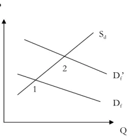
Figure 3.1 explains the increase in exports as the domestic currency depreciates. The figure shows the domestic export market. D_f represents the foreign demand for the domestic ex-port and Sd is the domestic supply of exports. Both the curves are expressed in terms of the

domestic currency. Equilibrium (1) where Df intersect Sd shifts when there is depreciation

in the domestic currency. When the deprecation occurs the Df curve will move upwards to

D_f ’ since the exports becomes cheaper for the foreign market. The foreign currency is worth more in terms of the domestic currency i.e. the demand increase. The economy will end up in a new equilibrium (2), where Df ’ intersect Sd where both the domestic price (P)

and the quantity (Q) have increased (Salvatore, 2004).

Figure 3.1 shows the effect on domestic exports due to depreciation of the domestic currency Source: Salvatore, 2004

3.2 Marshall-Lerner condition

The Marshall-Lerner condition verifies whether the foreign exchange market is stable or unstable. Conclusions that can be drawn from the Marshall-Lerner condition is depending on the shape of the curves for the demand for import and exports in a country. The condi-tion indicates that the foreign exchange market is stable if the sum of the price elasticity’s of the demand for imports and exports are greater than one, in absolute terms. It is better for the country if the two elasticity’s exceed one by a large amount since the current ac-count then improves more in case of a depreciation. If the price elasticity’s sum up to less than one in absolute terms, the foreign exchange market is unstable. The current account will be unaffected by a change in the exchange rate if the elasticises sum up to exactly one, in absolute numbers (Salvatore, 2004). If the Marshall-Lerner condition holds depreciation will improve the current account (Gärtner, 1993).

The reasoning behind the use of the Marshall-Lerner condition is to examine if the foreign exchange market is stable or unstable. The exact shape of the demand and supply curves of the foreign exchange market is hard to determine and it is therefore hard to determine if the foreign exchange market is stable or unstable. If the supply curves could be determined it would be straightforward to correct a deficit in the current account by deprecating the currency (Salvatore, 2004).

Policymakers today are taking the responsiveness of trade flows to relative price changes into account when constructing an exchange rate policy or a commercial policy.

2 1 Sd Df’ Df Q P

cally, the elasticities of the demand for imports and exports had a bigger impact and were used more frequently by policymakers in order to make a decision (Bahmani-Oskooee and Niroomand, 1998).

The sum of the elasticities for the demand for imports and exports would need to be suffi-ciently larger than one so that the supply and demand curves of the foreign exchange rate are elastic enough and depreciation can therefore make it possible to correct a balance of payments deficit. This is the reason why it is important to calculate the real world value of the price elasticity’s of the demand for imports and exports (Salvatore, 2004).

3.3 The J-curve effect

The Marshall-Lerner condition is assumed to hold in the long run. The current account may however at first decrease after a deprecation before the effect from the Marshall-Lerner condition kicks in and starts to improve the current account. This development of the current account is called the J-curve effect or the J-curve phenomenon, since the situa-tion resembles the letter J in a graphical sketch which can be seen in Figure 3.2 (Gärtner, 1993).

Figure 3.2 Sketch of the J-curve effect, t0 is the time of depreciation

Source; Gärtner, 1993

It is first in the medium run after a depreciation that the current account is expected to im-prove, since it takes time for the importers and exporters to adapt to the new relative prices. Depreciation affects the current account through three different channels;

1. Immediate response; the prices and volumes are fixed through contracts that were stated before the depreciation, so the importers and exporters can not change their behaviour. The current account worsens, since more domestic currency has to be paid for imports that have a fixed price and volume. However, this does not occur if the contracts are fixed in domestic currency but this rarely happens.

2. Medium-run response; the new contracts that are set reflect the new relative prices that are in favour of the domestic products. This change in price shifts the demand to domestic products from foreign products. The current account starts to improve after the shift in demand takes place. This can occur soon after the deprecation but the full effect might take several years.

t Current account

Current account

3. Long-run response; the only way for the prices to be unaffected by the increase in de-mand is if the domestic country experiences an extreme situation of unemploy-ment. If the price elasticity of the domestic goods supply is finite, higher prices are a consequence from higher export volumes, thus the current account continues to improve. The comparative advantage that was gained by the deprecation becomes smaller because of the price increase. The new long-run level is above the initial long-run level (Gärtner, 1993).

The J-curve can also be explained by elasticities. If the price elasticities in absolute terms of export and import demand are high enough, the trade balance will rise in response to cur-rency depreciation and vice versa if it is low. In the J-curve effect the elasticities are low di-rectly after depreciation. The initially low elasticities can be explained by the fact that it takes some time to change input patterns in the production (Hacker and Hatemi-J, 2003). The J-curve effect can also arise from differences in import and export prices. The domes-tic currency price of imports normally rises faster than prices of export after a depreciation which leads to small changes in the quantities. Gradually, the quantity of exports will rise and the quantity of imports fall, export prices catch up with import prices so that the coun-try’s national trade balance becomes positive (Salvatore, 2004).

The evaluation and examination of the J-curve is important for several reasons. First, it provides an indirect test of the Marshall-Lerner condition. Second, it provides crucial in-formation for trade and exchange rate policy decisions, since it gives an approximation about the length and depth of the deterioration in the trade balance after depreciation (Demirden and Pastine, 1995).

The relationship also gives information concerning the current account. A current account that is either too large or too small is undesirable, due to the associated problems with suboptimal intertemporal trade situations. Policymakers are also interested in knowing if the trade balance is on a level that can be estimated to be optimal. The policymakers can easier reach the targeted trade balance at their time scale if they know how the exchange rate affects the trade balance in the long run. The policymakers might also gain important insights on the national income in the short run and can therefore help them target the op-timal level of the national income (Hacker and Hatemi-J, 2004).

Some empirical studies confirm the existence of the J-curve effect. The studies found that the elasticities in the long-run experienced today are approximately twice as high as those in the 1940s. The reason behind this rise is that real-world elasticities are high enough for sta-bility to be expected on the foreign exchange market in the short run. It also reflects that demand and supply schedules for the foreign exchange in the long-run are fairly elastic. However, in the very short run i.e. roughly six months, deterioration in the current account is found directly after depreciation due to the fact that the elasticities are small and after that an improvement occurs i.e. the J-curve effect. The foreign exchange market is unstable in the very short run (Salvatore, 2004).

There have also been studies in which the J-curve effect cannot be found. For small open economies the J-curve effect may not exist, this holds true especially in the short-run (Hsing, 2005). The long-run effect is also dependent upon other variables such as; domestic spending, international competitiveness of tradable goods and changes in the terms of trade which also affects the J-curve effect (Bahmani-Oskooee et al, 2005).

In the study made by Hacker and Hatemi-J (2003) empirical evidence is provided for the existence of the J-curve effect in Sweden along with four other small countries in the north

of Europe. They also found that the export-import ratio often converge to a higher long-run equilibrium.

The J-curve effect is assumed to arise from the existence of already made contracts. How-ever, most developed countries today have their nominal trade balance, import prices and export prices expressed in terms of a foreign currency. In this case, the prefixed contracts cannot be a factor that explains the J-curve. When a country uses foreign exchange rate to express their own nominal trade balance, the J-curve effect can instead be explained by the degree of exchange rate pass-through and the short-run price elasticities of export and im-port demands. The scale of the J-curve is dependent upon the short-run degree of pass-through; the scale becomes larger as the degree of pass-through increases (Han and Suh, 1996).

3.3.1 Exchange rate Pass-Through

The degree of pass-through from the exchange rate to export prices can be defined as the percentage by which export prices, measured by the home currency, rises when the home currency depreciates. The same can be done for pass-through from the exchange rate to import prices (Han and Suh, 1996).

The degree of pass-through from the nominal exchange rate to export prices, which is measured by the foreign currency, might be different whether the home country’s currency appreciates or deprecates (Han and Suh, 1996).

The pass-through from depreciation to domestic prices may be less than complete, which implies that the increase in the domestic price of the imported commodity may be smaller then the depreciation. This means that for example a ten per cent depreciation in the do-mestic currency account may result in an increase in the dodo-mestic price of the imported commodity that is less than ten per cent. The reason behind this is that foreign firms are very cautious about their market share in a country and are not willing to lose it by raising their export prices by too much. The start up costs are very high: it is very costly to plan and build or dismantle production facilities or to enter or leave a market. The firms absorb the price increase, to a certain extent, by lowering their profits. This is called the beachhead effect and is a sunk-cost model. The exporting firms might also believe that the deprecia-tion is temporary and are therefore reluctant to increase the price by the full amount (Salvatore, 2004).

Sunk-cost models are models that explain why it might be optimal for a firm to not pass-through an exchange rate movement to its domestic currency export price. It also explains why firms continue to supply markets even if the exchange rate movement is unfavourable. These models predict a slow adjustment of both trade quantity and prices which is referred to as trade inertia. Trade inertia is an exogenous variable and can be seen as a “memory”. There are several forces that may contribute to trade inertia such as: the time it takes for the market to clear, the time it takes for tastes to change and the time it takes for the trade contracts to resolve (Vesala, 1992).

The sunk-cost models are based upon the observation that sunk costs are crucial for the decision making in a firm and it yields hysteretic results i.e. temporary shocks leaves per-manent effects. One of the implications in the sunk-cost models is that the firm can use a “wait and see” strategy: they remain in the current state and as time passes they receive more information so that they can make a more accurate decision. If the exchange rate changes to a large extent, firms will enter or exit the market depending on the direction of

the change and as a consequence the total supply will change as well. The change in the ex-change rate (temporary shock) leaves a permanent effect, since the firms will not re-enter or exit the market if the exchange rate moves back to its initial state i.e. the effect is hyster-etic. The sunk-cost model explains why trade patterns can be unaffected by small changes in the exchange rate (Vesala, 1992).

When a country is small and open, its import prices are fixed, even if the country’s cur-rency depreciates since they are price takers on the international market. The degree of pass-through to import prices will always be one, measured in the domestic currency. The degree of pass-through in exports is therefore the factor that determines the value effect on the trade balance. For these countries the pass-through from the exchange rate to export prices will be more accurate. The mark-up and the cost proportion of imported material, measured by the home currency, in the production of exported goods are two factors that influence the pass-through. The pass-through is equal to one if the mark-up is fixed, and is equal to zero when the mark-up changes by the same proportion as the exchange rate. If the degree of pass-through is small there is little room for lowering the export prices, which happens if the cost proportion of imported materials are large (Han and Suh, 1996).

If a country would experience perfect “zero-pass-through” the domestic export price would increase and the domestic import price would stay at the same level in case of de-preciation. This yields an increase in the trade balance. If a country instead experiences per-fect pass-through, the domestic import price would increase and the domestic export price would stay the same leaving the country with a decrease in the trade balance (Hsing, 2005). The degree of pass-through might be large in the short run, when depreciation occurs. The degree of pass-through will however decrease and becomes smaller in the long run since the cost pressure increases. Due to differences in degrees of pass-through and short-run dynamics, the absolute size of the effect on nominal trade balance from an exchange rate movement will be different whether the currency depreciates or appreciates. This results in different dynamic paths. The size and the degree of intervention of exchange rate policies should therefore be different whether the domestic currency is deprecating or appreciating (Han and Suh, 1996).

3.4 Effects of Exchange Rate Volatility That Can Be Positive

or Negative

Real exchange rate volatility influences profitability, rents and the purchasing power to a large extent. However, the export volume has stayed almost at the same level while the ex-change rate volatility has increased by a large amount. Hence, the larger part of these trans-fers is made between one agent to another and one should be indifferent to such transtrans-fers (Manzur et al., 1992).

Ethier (1973) found that exchange rate uncertainty influences only the degree of forward cover and not the amount of international trade when a firm knows how their revenue will be influenced by future exchange rate. However, uncertainty towards how the firm’s reve-nue depends on future exchange rate will make the level of trade sensitive to exchange rate volatility and will reduce the level of trade and increase the terms of the trade-off of ex-pected profit for a reduction in risk. These factors will be less significant if the firm is en-gaged in massive speculations.

Firms are able to plan their production and exports using the forward exchange rates. Firms will then behave as profit maximisers, using the fully covered marginal profit as a

planning equivalent, even if the firm may not cover the whole exchange rate risk. Thus, the exchange rate volatility has no effect upon international trade (Baron, 1976b).

An exporter that is facing uncertainty in a market can eliminate this risk completely if there is an unbiased forward/futures market, or another financial asset, that is perfectly corre-lated to the spot price of the underlying asset. A problem arises since not all currencies or commodities are traded in forward/futures markets. Even if there does not exist any finan-cial asset that is perfectly correlated, the firm can reduce the risk if there is a finanfinan-cial asset that is highly correlated to the foreign exchange rate and is traded on the forward/futures market (Broll et al, 2001). When a firm is using alternative forward/futures contracts, the firm is conducting indirect hedging. The firm can gain an acceptable hedge by using this indirect instrument if the stochastic relationship remains stable over a time period. An in-ternational firm can benefit from indirect hedging in case of exchange rate uncertainty (Broll et al, 1995).

3.5 Negative Effects of Exchange Rate Volatility on Exports

International firms are of great importance in the world economy; they have an important role as importers and exporters and are involved in international capital flows. The future profit for a firm that arises from international trade and foreign direct investment (FDI) becomes uncertain by exchange rate volatility (Broll, 1994).

Exchange rate volatility has a negative effect upon world trade, since it increases the risk involved in international trade. This holds true even if forward/futures markets exist, since forward/futures markets cannot completely neutralise this effect which is due to several aspects: there is a cost involved, a risk premium, in the forward/futures market and few currencies have well-developed forward/futures markets across a wide spectrum of maturi-ties. Even if a well-developed forward/futures market exists, the risk cannot be eliminated because exchange rate volatility affects exporting firms by different channels. Either by bringing a change in the amount received in terms of the domestic currency, or by bringing changes in the prices of the commodity exported in terms of the domestic currency which will affect the volume of trade. Both effects lower the profit for the exporting firm. The price of the commodity will be affected by a large number of factors such as; the market structure in which the firm operates, the policies of its competitors, the sensitivity of de-mand for its product to the exchange rate (elasticity), the extent to which consumers an-ticipate price changes and so forth. The price is sensitive not only to the spot price when the payment is due but to the behaviour of the exchange rate from the time the order is placed until the last unit is sold (Ethier, 1973).

When including both the import demand and the export supply of the market, the risk from exchange rate volatility can either be put on the importing firm or on the exporting firm. Contracts are normally set in the exporter’s currency, which causes the importing firm to bear the risk. An increase in the exchange rate volatility, and thereby the risk, will reduce the volume of trade, if the firms are risk averse. This holds irrespective of which agent that bears the risk; the exporting or importing firm. The price is however affected differently depending upon which agent that is bearing the risk; if it is the importing firm the price will fall as import demand falls. The price will rise if it is the exporting firm that bears the risk since the exporter will charge an increasingly higher risk premium. Ceteris paribus, as ex-change rate volatility increases, the imports as well as the market price decreases (Hooper and Kohlhagen, 1978).

Economic agents are unable to predict the domestic value of foreign transactions when there is exchange rate volatility. This leads to a greater uncertainty in international trade and investment. Since the cost and risk are enhanced, the international trade will decrease. The covering of exchange rate risk in a forward exchange market becomes more expensive when the volatility increases (Clark, 1973).

The willingness of a firm to engage itself in international trade is dependent upon the long-term prospects for profit in that activity. The firm is unable to make precise estimations of the domestic value of its foreign sales when the exchange rate is volatile. The unpredicted exchange rate volatility will cause the profit to change. If the exporting firm is risk-averse, the increased volatility in profit will reduce the volume of trade i.e. the supply schedules will shift up to the left. The exporting firm cannot predict the effect that the exchange rate volatility will have upon their foreign sales due to two main reasons; forward/future mar-kets in foreign currency are not developed enough or the firm might be uncertain of the value of the foreign exchange that it wants to cover. If perfect foreign exchange market ex-ists, the variability of profit that rises from exchange rate volatility could be reduced, but not completely eliminated (Clark, 1973).

When the decision to export is made, the present commitment of resources is valued against the future expected desired rate of return on these resources. The firm cannot pre-dict the foreign exchange rate when taking the decision of whether to enter or continue on the export market. Some of the transactions that determine the profitability of the export activities can be hedged to avoid risk on the forward market, but not all. The covariance between the foreign price and the exchange rate has an important influence on the amount of expected profit that the exporter will cover on a forward/futures market. If the covari-ance between the two variables is largely negative, the smaller is the need for a for-ward/futures market to reduce the variability in the profits. The negative correlation works as a stabiliser and reduces the negative effect of exchange rate volatility (Clark, 1973). Exchange rate or price volatility leads to an increased uncertainty which reduces the pro-duction and exports. The most important aspect of the financial market is therefore the possibility for firms to reduce currency or price risk, and the following impact on produc-tion and exports (Broll et al, 1995).

Baron (1976a) states that an exporter faces two types of risks, due to the exchange rate volatility: from the nature of the sales process and from the transaction risk resulting from converting revenue from one currency to another. The price can be set in the currency of the importer or the exporter, the profit of the exporter is however uncertain either way. The exporter faces transaction risk when converting the foreign currency into the domestic if the price is set in the importers currency. When the price is set in the domestic currency the exporter faces an uncertainty in the quantity demanded at the time the importer make the purchase.

The major currencies have experienced increased volatility ever since the fixed exchange rate regime was abandoned in the 1970s. Thus, international firms have been exposed to higher foreign exchange risk. A firm that is risk averse and has the opportunity to sell its commodity either on the domestic or foreign market experience export flexibility. The mul-tinational firms are considered to have export flexibility, since they make use of distribution facilities that exist all over the world. The firm can then take the future foreign exchange spot rate into consideration before choosing which market it should penetrate. The firm will export if it is profitable, but will then be exposed to exchange rate risk. This implies that the firm’s profit is not linear in the foreign exchange rate and that a forward/futures

contract cannot be used to form a perfect hedge. A more effective hedging tool is to write a European call option1_{. The major flaw with this approach is that it assumes that there is}

no risk premium involved in the price of the call option. So the firms will endure a cost as-sociated with the call option, which will make them reluctant to go forward with the export as the exchange rate volatility increases (Broll and Wahl, 1997).

Exchange rate volatility affects the optimal allocation of resources in a negative way which is due to the uncertainty in different variables such as profits. Exchange rate volatility might also influence trade flows in an indirect way; exchange rate volatility influences income volatility. Income volatility has an ambiguous effect upon trade, since it can reduce the trade through revenue uncertainty or increase the trade prospects by taking a real option perspective on the potential to establish operations in that market (Baum et al, 2001). Real exchange rate volatility is considered to be a source of uncertainty for risk averse ex-porters. The volatility of the real exchange rate affects the decision to export if the follow-ing assumptions hold: there is no possibility to construct a perfect hedge; this effect would be reduced if access to forward/futures markets existed and that the exporters are risk averse. Risk averse exporters choose to export less if the volatility increases and fewer re-sources will be allocated to the exporting sector (Gonzaga and Terra, 1997).

3.6 Positive Effects of Exchange Rate Volatility on Exports

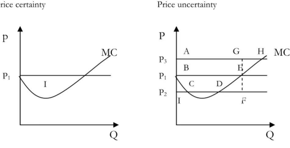
When a firm is profit-maximising and a price-taker in the output market, exchange rate volatility might increase exports. This is shown in Figure 3.3, where the marginal cost (MC), the price (P) and the output (Q) are represented. The left panel shows the scenario of a constant price and perfect predictability for the firm. The right panel shows the oppo-site: prices are fluctuating in a symmetric way, in this case between P2 and P3 where P3-P1=

(P2-P1)(De Grauwe, 1992).

In the left panel the area denoted by I represents the profit for each period when the fixed cost are excluded. In the right panel the profit will reflect the price it faces. If the price is low, (P2), the profit is smaller by the area represented by BEDI (BEFI-EFD) than the

profit in the case of price certainty. If the price is high, (P3), the profit is larger than the case

of price certainty by the area represented by BEHA (BEGA+EGH). The profit will be lar-ger on average if the price is fluctuating since the area BEHA is larlar-ger than the area repre-sented by BEDI. The difference in profit between price certainty and price uncertainty is shown by the areas EGH and DEF (BEHA-BEDI) in the right panel. Thus, the firm will increase its output and the profit if the price is high, since the revenue is higher per unit of output. The opposite will happen if the firm faces a low price, but a fall in price reduces profit not as much as the increase in profit due to an equivalent price increase. If P2 and P3

randomnly occur with equal propability, expected profit will be higher than if price was al-ways at P1 despite the fact that the expected price is the same (P1) in both cases. Even

though this is a simplified model, the result is the same as in a more complex model that includes imperfect competition and adjustment costs (De Grauwe, 1992). The higher ex-pected profits in the volatility price situation may induce firm entry if the deterrence from the additional risk is sufficiently weak.

1 _{A European call option gives the right to buy an asset, the option can only be exercised at maturity (Melvin,}

Price certainty Price uncertainty

Figure 3.3: Profits of the firm under price certainty (left) and uncertainty (right) Source: De Grauwe, 1992

Exchange rate volatility does not only represent a risk for a company, it also represents an opportunity to make a profit. When the volatility increases, it increases the opportunities of making large profits. One can see exporting as an option. A firm uses its option to export if the exchange rate is favourable, and the firm chooses to not use its option if the exchange rate is unfavourable. According to option theory the option value increases along with the variability of the underlying asset. Hence, a firm that has the option to export is better off if the exchange rate is volatile (De Grauwe, 1992).

Exchange rate volatility can positively affect the value of exporting firms through the price and volume impacts of exchange rates. It can also create more incentive for the exporting strategy compared to the one of FDI. This is due to the fact that the comparative advan-tages a firm can gain from exports become relatively more attractive when exchange rates become more volatile. An export-based strategy seems to be relatively more valuable than a FDI investment. Thus, investment in export production capacity could be a positive func-tion of exchange rate volatility. The adjustment cost and the cost of financial distress are omitted (Sercu and Vanhulle, 1992).

The exchange rate volatility increases the value of the export strategy and the value of ex-porting for firms that experiences comparative disadvantage in international trade and fol-lows a stationary bang-bang policy of entry and exit. A stationary bang-bang policy of entry and exit can be seen as an all-or-nothing strategy. The firm either totally ignores the market and stays out of it or totally commits to the market and enters; this policy can be seen as natural since the optimal policy is not known. The value of the export strategy and the value of exporting increase due to the fact that the expected cash flows from exporting grow faster than the associated entry and exit costs. A firm that experiences comparative disadvantage in international trade is facing a loss when exporting when the exchange rate equals the parity rate at which internationally traded commodities are equally expensive in the domestic market as in the foreign market. To enter a foreign market an exporting firm faces costs. If the firm stops exporting, the firm will face exit costs. Whether the expected export volume for a firm will grow with exchange rate volatility depends on the optimal export volume being a function of the exchange rate and the optimal adjustment of entry and exit rates. Firms will on average enter sooner and exit later when the volatility

I H F B G C E MC P2 P3 D A C P1 Q P MC I P1 Q p

creases, so the number of trading firms will on average increase and by this also the average trade. Hence trade benefits from exchange volatility (Franke, 1991).

According to Sercu (1992) so can exchange rate volatility on average increase trade since it implies a higher probability that ex post deviations from the Commodity Price Parity will be larger than tariffs and transportation costs. This assumption is based upon the facts that a firm’s exposure can be replicated and hedged by standard options, the existence of per-fect competition and complete monopoly. The same result cannot be found in general if the assumptions are relaxed, but neither can it be ruled out.

4 Empirical Analysis

In this section the model will be put forward and examined. The variables in the model and the data will be explained. The data will partly be explained by a graphical interpretation where the relationship between the exchange rate volatility and export is examined. This will be followed by an evaluation of the model using regressions. The Granger causality test will be examined.

4.1 Model

The model that will be used in the empirical analysis is based on the following export equa-tion (4.1); t t t t t REER Y I V X =

α

β

β

β

β

ε

where αis the intercept, X is the volume of exports in Sweden, REER is the real effective exchange rate index for Sweden, Y is the total volume of the Swedish industrial production, I is the total import in the Euro zone for consumption goods, V is a measure of exchange rate volatility and ε is the stochastic error term.

The real effective exchange rate index is calculated for the Swedish krona using the real ex-change rate between the Swedish krona and other currencies. The different currencies have different weight in the index and this weight is calculated from the consumer price index in the two countries and their bilateral nominal exchange rate. A rise in the variable REER represents a real appreciation of the Swedish krona. Y, the total volume of the Swedish in-dustrial production and can be seen as a “push” factor for the Swedish export, I represents the total import in the Euro zone for consumption goods and can be seen as a “pull” fac-tor.

The coefficient β1 is expected to be negative i.e. if the real effective exchange rate index is

increasing the country experiences appreciation and the commodities in the home country become relatively more expensive and economic agents will change their behaviour. The economic agents on the foreign market will choose domestic commodities since they are relatively less expensive. Hence, their import will decrease. The coefficient β2 is expected to

be positive since the exports increase if a “push” factor becomes stronger. If the Swedish production increases it will have spill-over effects on the export since the Swedish market is filled and a company has to go abroad to find a market for its commodities. The coeffi-cient β3 is expected to be positive since exports increases if a “pull” factor becomes

stronger i.e. if the imports in the Euro zone increases the exports for Sweden will increase since Sweden to a large extent exports to the Euro zone. The coefficient β4 of the variable

V, the exchange rate volatility is however ambiguous.

The measure of the exchange rate volatility will be calculated using the variance of the ex-change rate for five periods; the two periods before, the period examined and the two peri-ods after. For example: when calculating the volatility for the month March the variance for the months January, February, March, April and May will be used. One can also calcu-late the volatility for a month by using the daily figures and take an average of those. The reasoning behind the chosen method is that the exchange rate is influenced by the expecta-tions of what will happen in the coming periods and by events in the past periods.

The data are from between the years 1993 and 2006. The reason for the chosen period is that the Swedish currency started to float in November 1992. While investigating the

rela-tionship between exchange rate volatility and export a floating exchange rate regime is needed in the specific country since the exchange rate is allowed to fluctuate.

4.2 Graphical interpretation

In this section graphs will be used to interpret whether one can see a relationship between the exchange rate volatility and the exports. It also shows the characteristics of the chosen data. This is done as a complement to the regression analysis that follows in the next sec-tion.

The following Figure 4.1 shows total exports on a monthly basis for Sweden between the years 1993 and 2006. The main trend in exports, represented by the straight line, has been increasing through the years. Exports have been fluctuating around this trend.

Aggregated Exports for Sweden between 1993-2006 0 20000 40000 60000 80000 100000 1 9 9 3 M 0 1 1 9 9 4 M 0 3 1 9 9 5 M 0 5 1 9 9 6 M 0 7 1 9 9 7 M 0 9 1 9 9 8 M 1 1 2 0 0 0 M 0 1 2 0 0 1 M 0 3 2 0 0 2 M 0 5 2 0 0 3 M 0 7 2 0 0 4 M 0 9 2 0 0 5 M 1 1 Time T o ta l a m o u n t Export Time trend s

Figure 4.1: The total aggregated export in Sweden between 1993 and 2006. Source: Statistics Sweden(Statistiska Centralbyrån).

Exports are growing over time which is consistent with applied theory and the reality of many countries. Even if the export is fluctuating it does not move extensively around the main core. Seasonality should not be found in the data since it has been adjusted for by the database. However some patterns can be seen in the later years, 2000 and onwards. By cal-culating the average for the months in all of the years, one can see if there are months that clearly distinguish themselves by having very high or very low values. When using all of the years October and November distinguish themselves from the other months. Since some patterns can be seen from the year 2000 and onwards, calculations were made for these years. In the later case the months March, October and November distinguish themselves from the other months.2

2 _{To get rid of the problem of seasonality one can include dummy variables in the regression analysis for the}

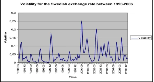
Figure 4.2, shows volatility in the exchange rate for the $/SEK between the years 1993 and 2006 this data is also on a monthly basis.

Volatility for the Swedish exchange rate between 1993-2006

0 0,05 0,1 0,15 0,2 0,25 0,3 1 9 9 3 0 3 1 9 9 3 1 2 1 9 9 4 0 9 1 9 9 5 0 6 1 9 9 6 0 3 1 9 9 6 1 2 1 9 9 7 0 9 1 9 9 8 0 6 1 9 9 9 0 3 1 9 9 9 1 2 2 0 0 0 0 9 2 0 0 1 0 6 2 0 0 2 0 3 2 0 0 2 1 2 2 0 0 3 0 9 2 0 0 4 0 6 2 0 0 5 0 3 2 0 0 5 1 2 Time V o la ti li ty Volatility

Figure 4.2: The Swedish exchange rate volatility between 1993 and 2006. Source: Statistics Sweden(Statistiska Centralbyrån).

Volatility does not follow any seasonal pattern. Hence, seasonality is not a problem in ei-ther of the variables. Volatility does not have a trend that grows or decreases over time. However, one can see that the volatility is often higher since the year 2000.

There is no relationship to be found when comparing the two graphs. It is obviously hard to see a clear-cut relationship between the two variables in these figures due to the high frequency of the data.

4.3 Regressions

Three regressions will be presented in this thesis. The independent variables will be lagged in some of the regressions. By using the Schwarz information criterion, where it is mini-mised, the most appropriate number of lags was found. The reason for the use of lags is that the dependent variable is often influenced by the independent variables with a time lapse e.g. it takes time for the export to adjust to the new exchange rate since contracts have to be changed and the already made contracts hinder the companies to change their behaviour instantaneously.

A unit root test was conducted to verify if the data exhibited non-stationarity or stationar-ity, using the Elder and Kennedy (2001) approach. The only variable that was non-stationary was the industrial production in Sweden. The two variables Swedish exports and the import for the Euro Zone were trend stationary. A more detailed explanation of the unit root test can be found in the appendix.

The chosen data are gathered from different databases. From OECD the data for the real effective exchange rate index was collected. The industrial production in Sweden was from the Statistics Sweden (SCB). The import from the Euro zone was collected from the Euro-pean Central Bank (ECB). The data for the first three variables were found in the Ecowin, which is a database that collects data from different sources. From the Statistics Sweden (SCB) Swedish exports data were collected and the exchange rate was found in the Swedish

central bank’s database. The data found are already adjusted for seasonality so it is there-fore no need to correct it further.

The variables in the first regression are transformed into growth using equation (4.2):

Growth= ( Xt-X t-1)/ X t-1 (4.2)

The first regression includes all the variables and all of them are transformed into growth represented by the ^. The volatility variable is logged. All the variables are also lagged by one period to include the effect from one previous period, upon the dependent variable. The choice of one period was based on the Schwarz information criterion. Equation (4.3) is used: t t t t t t t t t t REER Y LogV REER Y I LogV X =α+β +β +β Ι +β +β +β +β +β − +ε ∧ − ∧ − ∧ − ∧ ∧ ∧ ∧ ∧ ∧ 1 8 1 7 1 6 1 5 4 3 2 1 (4.3) The result is found in the following Table 4.1:

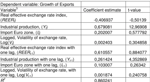
Table 4.1. Result from first regression (equation 4.3)

Dependent variable: Growth of Exports

Variable3 Coefficient estimate t-value

Real effective exchange rate index,

(REERt) -0,406937 -0,50139

Industrial production, (Yt) 0,679081 12,96908

Import Euro zone, (It) 0,202007 0,577792

Logged, Volatility of exchange rate,

Log(Vt) 0,002403 0,304858

Real effective exchange rate index with

one lag, (REERt_-1) 0,610557 0,884077

Industrial production with one lag, (Yt-1) 0,261424 4,352869

Import Euro zone with one lag, (It-1) 0,103007 0,26342

Logged, Volatility of exchange rate, with

one lag, Log(Vt-1) 0,001874 0,240758

R2 _0,860241

3 _{All the explanatory variables are in terms of growth, calculated as in equation 4.2}

The coefficient estimates of the variables: industrial production in Sweden at time t and at time t-1, which represent the current and the previous period, were significant at the five percentage significant level, since their t-values were above two in absolute terms. The in-dustrial production in Sweden had the expected sign in both cases. R2 _{is approximately 86}

per cent i.e. 86 per cent of the variance in the dependent variable can be explained by the model.

In the first regression the coefficient estimates of the volatility and the volatility with one lag were not significant, not even at a ten percentage significant level. Both the coefficients did have a positive sign which is interpreted as an increase in exports if volatility increases. The coefficient estimate for the variable industrial production in Sweden is expected to be positive since it is considered to be a “push” factor. The Swedish market’s demand for the commodities that are produced by the Swedish firms are too small to satisfy the supply from the Swedish firms.

In the second regression the level values of the variables are used. All the variables are logged so the results can be interpreted as percentage changes and hence the scales of the variables are not needed to take into account. The industrial production in Sweden is not included in this regression since it was tested to be non-stationary. A time variable is in-cluded to verify if export is growing over time. The equation (4.4) is used:

t t

t t

t LogREER Log LogV t

LogX =

α

β

β

β

β

ε

The result is found in the following Table 4.2:

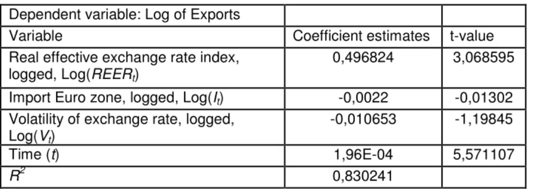
Table 4.2. Result from the second regression (equation 4.4)

Dependent variable: Log of Exports

Variable Coefficient estimates t-value

Real effective exchange rate index, logged, Log(REERt)

0,496824 3,068595 Import Euro zone, logged, Log(It) -0,0022 -0,01302

Volatility of exchange rate, logged, Log(Vt)

-0,010653 -1,19845

Time (t) 1,96E-04 5,571107

R2 _0,830241

The real effective exchange rate index and the time variable have significant coefficient es-timates at the five percentage significant level, since they have a t-value above two in abso-lute terms. The real effective exchange rate index does not have the expected sign for its coefficient estimate. The time variable on the other hand has the expected sign. R2_is

ap-proximately 83 per cent.

The coefficient estimate of the logged volatility was not significant and exhibits a negative sign i.e. volatility decreases exports. The coefficient estimate of the volatility had in this re-gression a higher t-value than in the other rere-gressions presented in this paper.

The coefficient estimate real effective exchange rate index was in this case positive which can be explained by the fact that it takes some time for economic agents to change their behaviour when the economic environment changes. The coefficient estimate for the vari-able time is positive which indicates that the level of exports is growing over time.

The third regression is also based on the level values and all of the variables are logged. All of the variables are also lagged by one period. This regression is also examining the Granger causality by including the export variable, with one lag, at the right side in the equation. This variable takes into account omitted variables. A time variable is also included to verify if exports are growing over time. The equation (4.5) will be used:

t t

t t

t

t LogREER LogI LogV LogX t

The result is found in the following Table 4.3:

Table 4.3. Result from the third regression (equation 4.5)

Dependent variable: Log of Exports

Variable Coefficient estimates t-value

Real effective exchange rate index, logged, with one lag, Log(REERt_-1)

0,22467 1,533161 Import Euro zone, logged, with one lag,

Log(It-1)

0,064009 0,431334 Volatility of exchange rate, logged, with

one lag, Log(Vt-1)

0,001366 0,174199 Export, logged, with one lag, Log(X t-1) 0,456934 6,375282

Time (t) 8,79E-05 2,591853

R2 _0,865646

The coefficient estimates of the variables lagged exports and time are significant at the five percentage significant level, since they have a t-value above two in absolute terms. Both of the two variables have the expected sign. R2_{is approximately 86 per cent.}

The coefficient estimate of the volatility when it was both logged and lagged by one period had a positive sign i.e. volatility increases exports but was not significant. This result re-sembles to the first regression where the coefficient estimates of the volatility, in the cur-rent period and the previous (one lag), was positive.

The coefficient estimate for time was also in this regression significant and positive which indicates that the level of exports is growing over time. The fact that the coefficient esti-mate of the lagged exports was positive can be interpreted as a positive correlation i.e. a positive value will be followed by a positive value.

The difference between regression two and three is that the third regression uses the vari-ables with one lag and includes the lagged exports. The result from the two regressions dif-fers however. The coefficient estimate for exchange rate volatility has opposite sign in the two regressions: it is negative in the second regression and positive in the third. This could be due to the fact that the third regression takes the time aspect into account, uses variables that are lagged by one period.

4.3.1 Granger Causality Test

Even though regression analysis can indicate a relationship of dependence on one variable upon another variable it does not need to imply causation. However, dealing with time se-ries the situation might be different. If one event happens before another it is possible that the first event is causing the second event, the reverse is however impossible, the later event cannot cause the first one. This is the reasoning behind the Granger causality test. This test relies upon the assumption that the relevant information for the prediction of the respective variables is contained purely in the time series data on these variables. If for ex-ample the variable X causes variable Y then changes in X should precede changes in the variable Y since the future is unable to predict the past. If past values of X significantly im-prove the prediction of Y, in a regression where Y is the dependent variable and has inde-pendent variables that include its own past values than one can draw the conclusion that X causes Y (Gujarati, 2003).

The equations that will be used for testing Granger causality in the current context are the following: t t t t X Y t X =

α

β

β

β

ε

α

β

β

β

ε

The variables that were tested were: export causes the volatility and vice versa, export causes industrial production and vice versa, export causes the import from the Euro zone and vice versa and export causes real effective exchange rate index and vice versa. This test is a complement to the third regression (equation 4.5) that also checks for Granger causal-ity. The result is shown in the following Table 4.4:

Table 4.4. Results from the Granger causality test

Causal Relation * Coefficient estimates t-values

Export →volatility 0,003874 0,832757

Volatility → export -0,76354 -0,15345

Export → industrial production in Sweden 0,384953 5,733922

Industrial production → export -0,43267 -3,0236

Export → import from the Euro zone -0,45336 -1,37648 Import from the Euro zone → export 0,018043 1,062271 Export → the real effective exchange rate index 0,057036 0,089508 Real effective exchange rate index → export -0,00315 -0,32195

*_{The symbol, →, represents the direction of causation, e.g. X →Y means that X causes Y. The associated}

co-efficient estimate indicates the degree to which it is true, and the t-value is used to test whether lack of that causality can be rejected.

There could not be found any causality in either direction between the variables: export and volatility, export and the import from the Euro zone or from the export and the real effec-tive exchange rate index. Between the variables export and the industrial production causal-ity was found in both ways and with negative signs.