Master
's thesis • 30 credits
The Demand for Wine in Sweden
-
an Econometric Approach
Swedish University of Agricultural Sciences
The Demand for Wine in Sweden – an Econometric
Approach
Johanna Widborg
Supervisor:
Examiner:
Yves Surry, Swedish University of Agricultural Sciences, Department of Economics
Jens Rommel, Swedish University of Agricultural Sciences, Department of Economics Credits: Level: Course title: Course code: Programme/Education: 30 credits A2E
Master thesis in Economics EX0907
Agricultural Economics and Management Master's Programme 120,0 hec
Course coordinating department:Department of Economics Place of publication: Year of publication: Title of series: Part number: ISSN: Online publication: Key words: Uppsala 2019
Degree project/SLU, Department of Economics 1242
1401-4084
http://stud.epsilon.slu.se
alcohol, demand system, elasticities, fixed effect, Sweden, wine economics
Abstract
This study uses a Linear Almost Ideal Demand System and a Single equation model, to study the demand for varieties of wine in Sweden. The data used in the study is open source sales data from monopolized alcohol store, Systembolaget, the majority of total sales of alcohol is bought at Systembolaget. It is shown that the two models give somewhat ambiguous results, however the results from the Linear Almost Ideal Demand System indicates that Red wine is a necessity for Swedish consumers and that Rose wine and Sparkling wine are luxury goods.
Table of Contents
1 INTRODUCTION ... 1
1.1 Aim and delimitations ... 1
1.2 Structure of the report ... 2
2 THEORETICAL PERSPECTIVE AND LITERATURE REVIEW ... 3
2.1 Systembolaget – History of the monopoly ... 3
2.2 Previous studies ... 4
2.2.1 Taxation of alcohol – controlling the consumption ... 5
2.2.2 Consumption trends in Sweden ... 5
2.2.3 Is wine a luxury good or a normal good? ... 6
3 METHOD ... 7
3.1 Separability ... 7
3.2 Single equation model ... 8
3.2.1 Elasticities ... 9
3.3 Almost Ideal Demand System, AIDS ... 9
3.3.1 Elasticities ... 11
3.4 Model testing ... 11
4 EMPIRICAL DATA ... 13
4.1 Data management ... 13
4.1.1 Creating an agregated data set ... 16
4.2 Limitations ... 16
5 ANALYSIS AND DISCUSSION ... 17
5.1 Single equation model ... 17
5.2 LAIDS ... 18
6 CONCLUSIONS ... 21
REFERENCES ... 22
List of figures
Figure 1 Utility tree (Edgerton et al., 1996, p. 7) ... 7
Figure 2 Utility tree used in this study ... 8
Figure 3 Distribution of prices in 2009 for all five wine categories ... 14
Figure 4 Price distribution 2009, corrected for skewness ... 15
Figure 5 Price distribution 2010 ... 25
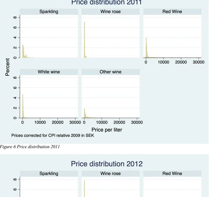
Figure 6 Price distribution 2011 ... 26
Figure 7 Price distribution 2012 ... 26
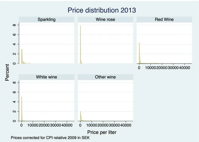
Figure 8 Price distribution 2013 ... 27
Figure 9 Price distribution 2014 ... 28
Figure 10 Price distribution 2015 ... 29
Figure 11 Price distribution 2016 ... 29
Figure 12 Price distribution 2017 ... 30
Figure 13 Price distribution 2018 ... 30
Figure 14 Price distribution 2010 - Corrected for skewness ... 31
Figure 15 Price distribution 2011 - Corrected for skewness ... 31
Figure 16 Price distribution 2012 - Corrected for skewnes ... 32
Figure 17 Price distribution 2013 - Corrected for skewness ... 32
Figure 18 Price distribution 2014 - Corrected for skewness ... 33
Figure 19 Price distribution 2015 - Corrected for skewness ... 33
Figure 20 Price distribution 2016 - Corrected for skewness ... 34
Figure 21 Price distribution 2017 - Corrected for skewness ... 34
Figure 22 Price distribution 2018 - Corrected for skewness ... 35
List of tables
Table 1 Descriptive statistics before outliers were removed ... 14Table 2 Descriptive statistics after outliers were removed ... 15
Table 3 Single equation model ... 17
Table 4 Parameter estimates ... 18
Table 5 AIDS - Price elasticities ... 19
1 Introduction
The past excessive demand for alcoholic beverages in Sweden is one of the reasons why Sweden has the monopolized alcohol store, Systembolaget. Since alcoholic beverages are a differentiated goods it is problematic to aggregate alcohol as one good, since the consumption patterns of spirits, beer and wine are different (Fogarty, 2006; S. Selvanathan & Selvanathan, 2005). In 1957 Systembolaget started a campaign to get Swedish consumers to switch
consumption from spirits to a less ethanol dense beverage, wine (Systembolaget, n.d.-d). The consumption shift from spirits towards beer and wine in the last twenty years in Sweden have been identified by Trolldal & Leifman (2018). The differences within each category of alcohol have also been widely studied, especially wine, which may be the most differentiated good within the category of alcoholic beverages because of the wide range of colors, origins, varieties and characteristics. Recent studies have used grapes as an instrumental variable (Cuellar & Huffman, 2008), or using expert critiques to investigate how customers respond to perceived quality (Dahlström & Åsberg, 2009). Others have used the wine’s origin to
investigate how it affects consuming behavior (Carew, Florkowski, & He, 2004; Davis, Ahmadi-Esfahani, & Iranzo, 2008; Friberg & Grönqvist, 2012). However, no other studies have studied the elasticities of demand solely within and across the colors of wine.
Using both a linear Single equation Model and a Demand System approach this study will investigate the demand elasticities within the differentiated good, wine. Wine is differentiated in the different varieties of wine: Sparkling, Rose wine, Red wine, White wine and Other wine, using open data from Systembolaget. Since the quality of the data was both highly specified but also missing some information used in other studies (Friberg & Grönqvist, 2012), such as degree of alcohol, the study has a more general approach than previous studies, focusing on the different variety of wine, but still manages to acquire new approaches toward the demand for wine in Sweden.
Since Sweden joined the European Union in 1995, and the state monopoly to import was dropped, the number of importing firms for alcoholic beverages has increased rapidly, resulting in a market where the consumer has more choice. The number of available choices for wine has been increasing, why it is interesting to seek for a better understanding of the demand for wine in Sweden. The objective of this research is therefore to examine the demand for wine in Sweden and acquire a greater understanding on how Swedish consumers allocate their spending within the differentiated good, wine. However, the demand for each wine at Systembolaget would have resulted in insignificant demand, why this study pools the data over the total sales of each variety of wine.
1.1 Aim and delimitations
The purpose of this study is to examine the demand for different varieties of wine in Sweden by using the self-reported price and sales data from Systembolaget. By estimating the demand system and the associated expenditure function, the study aims to find a more complete understanding of the characteristics of the demand for wine in Sweden. Yearly data collected from Systembolaget is used in the study, since the data is highly specific, the differentiation within the wine category can be made. No data from the consumption at restaurants, nor imported alcohol will be accounted for, in order to avoid measurement errors due to
time of the study, the income effects will, therefore, not be studied. Further limitations regarding the data is explained in the chapter of data management.
1.2 Structure of the report
This study will have the following structure: first, the method of both models used will be discussed and explained in Chapter Two. Second, in Chapter Three a historical background of Systembolaget will be discussed, to get a greater understanding of the nature of the Swedish alcohol monopoly. Furthermore, in Chapter Three, previous studies will be presented, reviewed and discussed. Third, the data management and the econometric methods will be explained in Chapter Four. Fourth, the results and their following discussion will be presented in Chapter Five. Finally, Chapter Six outlines a conclusion and discussion of further research.
2 Theoretical perspective and literature review
In the following chapter a brief background of the Swedish monopoly and an outline of how the Swedish monopoly is operating today. Which will be followed by a literature review focusing on alcohol demand with system approach, but also explaining the taxation of alcohol in Sweden and consumption trends.
2.1 Systembolaget – History of the monopoly
The Swedish monopoly of the distribution of alcoholic beverages have a history from the extensive alcoholic problems in the 19th century. However, the state-owned store for alcoholic beverages, Systembolaget, as we know it today dates back to 1955, when the state-owned country wide Systembolaget opened. Until Sweden entered the European Union in 1995, not only was the distribution a government monopoly but also the only firm allowed to import, called ‘Vin och Sprit AB’ (Systembolaget, n.d.-b).
Extensive criticism against Systembolaget started on New Year’s Eve 1991, and the
government subsequently started an investigation as a working ground for adjustments needed for the upcoming election for entering the European Union (Systembolaget, n.d.-f).
There were suspicions from the European Commission that Systembolaget and Vin och Sprit AB might discriminate among the imported goods. However, in 1994 the Commission found that the distributions in the stores all over the country were not discriminating. Vin och Sprit AB lost the monopoly status and from 1995 there are over one hundred importing firms. Systembolaget also lost the monopoly to distribute to restaurants in 1995, and restaurants can, therefore, import directly through any import firm (Systembolaget, n.d.-f).
In 2019, Systembolaget has 436 brand stores, outlets and customers can also order to approximately 470 local agents, such as a supermarket, without additional costs. The local agents can only distribute what is ordered by customers and have no stocks (Systembolaget, n.d.-c). Since 2012, Systembolaget has offered home delivery as a test to follow the consumer patterns of the citizens and increase the level of service especially for consumers with long distances to an outlet or local agent (Regeringskansliet, 2018). After reports of no increase in the alcohol consumption, the home delivery has been proposed to become part of the standard operating procedures for Systembolaget. The price setting and the access to alcoholic
beverages is the same in all stores and have no local variations.
In the outlets, the fixed range of different products is approximately 2,500 varieties, with the range in each store depending on the demand in each outlet. The fixed range represents 95% of the total sales. In addition to the fixed range, Systembolaget also has a range of products which are available to order both from the store but also from the internet and will be delivered to the outlet selected by the customer. This online range consists of around 13,500 items. Additionally, there is also a temporary range consisting of 1,500 items which consists of seasonal, small scale locally produced and exclusive range, with a relatively high price and in limited volumes. Consumers can also privately import from other countries through
Systembolaget (Systembolaget, 2018).
Besides the monopoly, there are multiple other instruments to control the alcohol consumption in Sweden. The two administrative instruments are limiting sales and
accessibility. Sales are limited through a strict non-tolerance towards encouraging additional sales and volume discounts, nor do they have any loyalty club. Furthermore, Systembolaget offers a return policy which provides the customer with the possibility to return what is
unopened and unconsumed. Accessibility is restricted through the limited number of
salespoints, opening hours and the age limit of 20 to purchase alcohol. The age limit to drink alcohol on premises at a bar or restaurant is the same as the legal age, 18 years
(Systembolaget, n.d.-e).
2.2 Previous studies
Previous elasticity studies study wine as a homogenous good in relation to spirits and beer or alcohol as a homogenous good in relation to other food stuff that is consumed at home (Fogarty, 2006; Mitchell, 2016; S. Selvanathan & Selvanathan, 2005). When making a Using a source-differentiated AIDS approach, Carew et al. (2004) studied the demand for table wine in British Columbia. The Canadian wine production is on the rise from a
monoculture within the wine sector in 1930-1980 towards a more diversified wine production with a large variety of grapes and wine. Carew et al. used the source differentiated AIDS model to estimate the differences in demand on domestic and imported Red and White wine. Assuming two stage budgeting process and weak separability between goods, they conclude that the demand elasticities are inelastic for most of the Red wines and White wine from British Columbia and Europe whereas the White wine from the rest of the world is elastic. They find substitute relations vary between wines of different regions.
Alley et al. (1992) also apply an AIDS approach on the demand for alcoholic beverages in British Columbia. Including six product categories, Wine produced in British Columbia, imported wine from US, other imported wine, also including other Canadian wines from outside British Columbia, beer, spirits and other goods. Using monthly sales data from April 1981 to August 1986 provided by the British Columbia Liquor Distribution Branch and a CPI for Vancouver as a price setting for other goods than alcohol.
With the main goal of reaching a greater understanding about the demand for Australian wines in the US, Davis et al. (2008) uses a nested logit model to explain the demand for wine under product differentiation. They argue that most of the AIDS models in previous studies have some flaws, meaning that the aggregating wine at product level and assuming restrictive markets makes them unsuitable to capture the true effects and the disequilibria. Also, the problem that most studies do not differentiate the different attributes of wine. Davis et al. uses sales data from groceries and drugstores over 3 consecutive years, 2003-2005. The data corresponds to approximately 52 percent of the total US sales, they selected the 50 top brands in the US market. Even though all 50 brands were not available in all stores they argue that this does not affect their analysis. They nested over quality and region of origin, the quality is defined by price segments, they argue that the price is a reasonable proxy for the quality of the wine. Davis et al. argues that wine knowledge is increasing with the quality, which creates a more homogenous group of consumers. The consumer in the lower qualities have less wine knowledge, in combination with a larger supply they are a much more heterogeneous group. Therefore, pricing is not the most efficient tool to compete on the US market of wine, since the consumers of the lowest qualities cannot differentiate as much as in the higher quality groups.
Gruenewald et al. (2006) have looked at quality substitutions and price elasticities for the different categories of alcohol in Sweden. The monthly data provided by Systembolaget let them account for seasonal sales differences and the number of public holidays and Fridays. Differentiating the complex good alcohol into high, medium and low quality, within each
category, beer, wine and spirits. Each quality account for one third of the total ethanol sales for each category. Their research shows how consumers substitute both between quality segments as well as between beverage categories. The results indicate that consumers are more likely to adapt to price changes by substitution rather than reducing their consumption. They conclude that an efficient way to decrease alcohol consumption would be to increase prices on low quality alcohol. However, Sundén (2019) argues that an increase on the low quality alcohol would add a threshold that would have an effect only on consumers who consumes the least expensive alcohol and not an effect that would decrease the consumption over all.
Ceullar et al. (2010) uses both a Fixed Effect Model and an instrumental approach to study the demand for wine in the United States. Using monthly data of 750 ml bottles from grocery stores from all over the US. Per capita disposable income is used as income variable over the years 2002-2005. Their instrumental variable is the grape price data provided by the
Californian department of Food and Agriculture. Grapes are the main ingredient in wine however they conclude that the grapes only account for 10 percent of the total price why their instrument might be questioned. The disaggregation made in the article is that wines are estimated by color and by the 6 most selling Red and White wines. They also make the distinction in price points below and above $10 which is a rather arbitrary chosen price. They found that Red wine drinkers are more willing to switch to White wines than White wine drinkers are to switch to Red.
2.2.1 Taxation of alcohol – controlling the consumption
There is no doubt that increasing taxation of alcohol will reduce the consumption, to which extent depends on the monitoring set in place by the government (Babor et al., 2010). Consuming alcohol has a large impact on multiple parts of the body and the economy, every year the consumption of alcohol contributes to over 3 million deaths, or approximately 5% of all deaths worldwide. The World Health Organisation (WHO) has launched an initiative to reduce the harmful use of alcohol by 10% by 2025 since the alcohol consumption in the world is increasing. Pricing, restrict or ban or increase the prices of alcoholic beverages are the most efficient intervention to decrease alcohol consumption and the core objectives of the initiative (World Health Organization & Management of Substance Abuse Team, 2018).
In Sweden the taxation of alcohol is differentiated between the beverage categories. From 2017-01-01 the tax levels for wine is untaxed below 2,25 percent and from 2,25 percent to 18 percent the tax is ranging from 9,19 to 54,79 kronor per liter (Skatteverket, n.d.). Over the time period of this study the tax levels for alcoholic beverages have changed 3 times, in 2011 they increased by 7 percent, in 2015 they increased by 9 percent and in 2017 they increased by 4 percent, for wine (Skatteverket, n.d.). This may have an effect on both prices and total sales which is not accounted for in this study due to the lack of data on ethanol level in the open data provided by Systembolaget.
2.2.2 Consumption trends in Sweden
The consumption trend according to self-reported survey data and sales data from Systembolaget indicate that the consumption of spirits is decreasing while the wine consumption is increasing. Beer on the other hand has had a rather steady level of
consumption for the last 10 years. Approximately 62,8 percent of the total consumption of alcoholic beverages is bought at Systembolaget and 13,5 percent is bought abroad. 10,2 percent of the alcoholic beverages are consumed at restaurants and bars. These estimations are based on a yearly survey with a randomly selected sample size of 1.500 people per month, in
total 18.000 participants who estimate their consumption the last 30 days (Trolldal & Leifman, 2018).
A number of measurement errors is connected to these estimations, since people tend to underestimate their consumption of alcohol. Multiple studies about alcohol address this problem and that policies concerning alcohol are based on potentially very biased data (Cook & Moore, 2000; Room, 2004). In a recent report about the Swedish sin taxes for alcohol, tobacco and gaming in terms of monetary games, the statistics is clearly questioned. The lack of consistent quality statistics makes it difficult to investigate the true effects of the policies and the true costs related to consumption of alcohol, tobacco and gaming (Sundén, 2019). How changes in foreign taxes affect the cross-price elasticities have been studied using municipality data on consumption and distance to borders as well as the number of outlets per capita. The results show that the demand for alcohol in Systembolaget’s outlets depend on the distance to neighboring countries with lower prices, resulting in reduced tax revenues for Sweden (Asplund, Friberg, & Wilander, 2007).
2.2.3 Is wine a luxury good or a normal good?
In the study by Lööv and Widell (2009) the AIDS model is used to estimate the demand for food in Sweden. Even if they exclude alcoholic beverages from their analysis, they still assume alcohol as a commodity group to be a luxury good. However other studies show that both wine and beer is considered as a necessity and only spirits should be considered as a luxury good (S. Selvanathan & Selvanathan, 2005). Fogarty (2009) makes it clear that wine is much more heterogeneous than both beer and spirits, why a classification of the category as a whole may lead to a misleading statement. In the study about price sensitivity for perceived quality in wine, Dahlström and Åsberg (2009) estimates that for some price segments of wine, wine is a luxury good.
Most studies within the field of wine economics and demand analysis it can be concluded that almost ideal demand system approach is more frequently than other demand systems, as previously mentioned. The available data for alcohol consumption in Sweden is rather scanty which might be surprising since the instruments for alcohol consumption in Sweden are strict compared to the rest of the world.
3 Method
The demand models used in this study is based on Neoclassical demand theory. Individuals are assumed to be rational and are always seeking to maximize their utility given their available income (Varian, 2010).
3.1 Separability
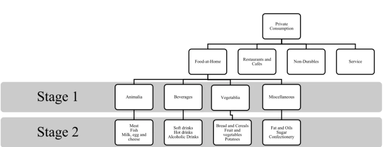
When estimating the demand for any good, the ideal demand system would include the consumption in relation to all expenditure, a complete demand system. However, this would require a large amount of data from different data sources in combination with thousands of equations which would be both very expensive and almost impossible. Making some a priori assumption of the consumer’s preferences is the most commonly used way of going about this problem. The assumption of a multi stage budgeting process and weak separability are two common assumptions (Edgerton et al., 1996). The two-stage budgeting process is explained as follows: ‘This approach implies that goods can be divided into a number of “separate” groups, where a change of price in a good in one group affects the demand for all goods in another group in the same manner.’ (Edgerton et al., 1996, p. 69). The two-stage budgeting process, Figure 1 implies that consumers in the first stage allocate the total expenditure for Animalia, Beverages, Vegetablia and Miscellaneous and in the second stage the allocate how much to spend on soft drinks, hot drinks and alcoholic drinks. Applying a separable demand system is logic since a consumer is more likely to compare the good with similar goods, rather than other goods or services.
Figure 1 Utility tree (Edgerton et al., 1996, p. 7)
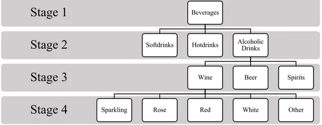
In the four-stage budgeting process applied in this study, Figure 2, is an extension of Figure 1 which resembles the one provided by Carew, et al. (2004). Where the third stage is the
decision of consuming wine, beer or spirits and the fourth stage which category of wine, Sparkling, Rose, Red, White or Other. The utility tree in Figure 2 also resembles the utility tree used in Edgarton et al. (1996, p. 206) for forecasting food consumption in Finland.
Stage 2
Stage 1
Private Consumption Food-at-Home Animalia Meat Fish Milk, egg andcheese Beverages Soft drinks Hot drinks Alcoholic Drinks Vegetablia
Bread and Cereals Fruit and vegetables Potatoes
Miscellaneous
Fat and Oils Sugar Confectionery Restaurants and
Figure 2 Utility tree used in this study
3.2 Single equation model
The estimated model is a Single equation Model applied on the pooled data inspired by Cuellar & Huffman (2008), since no instrumental variable is applicable the following model will be applied:
𝑙𝑛(𝑆𝑎𝑙𝑒𝑠()) = 𝛼(+ 𝛽𝑙𝑛(𝑅𝑃()) + 𝜃𝑇𝑖𝑚𝑒(+ 𝜀() (1)
Where 𝑖 is the variety of wine, 𝑡 is year, 𝑅𝑃() is the Real price, 𝑇𝑖𝑚𝑒 is the Single equation for year 𝑡 and 𝑆𝑎𝑙𝑒𝑠() = 𝑅𝑃() ∗ 𝑄𝑢𝑎𝑛𝑡𝑖𝑡𝑖𝑒𝑠().
𝑙𝑛(𝑆𝑎𝑙𝑒𝑠()) = 𝛼(+ 𝛽𝑙𝑛(𝑅𝑃()) + ∑=DEC 𝛿=𝐷𝑈𝑀=∗ 𝑙𝑛A𝑅𝑃=)B+ ∑C=DE𝛾=𝐷𝑈𝑀= + 𝜃𝑇𝑖𝑚𝑒( + 𝜇=+
𝑢() (2)
Where 𝜇= are other control variables, subscript 𝑗 = 1 is activated by Red, 𝑗 = 2 by Sparkling, 𝑗 = 3 by Rose, j=5 by White and 𝑗 = 5 by Other wine. 𝐷𝑈𝑀= is a dummy variable which
takes 1 for wine 𝑗 and zero otherwise.
Assuming the following fixed effects regression assumptions, notation from Stock and Watson (2015, p. 412):
1. 𝜀()/𝑢() has a conditional mean zero: 𝐸(𝜀() /𝑢() |RPRS, … , 𝑅𝑃(V, 𝛼() = 0 2. RPRS, … , 𝑅𝑃(V, 𝛼(, … , 𝛼V)Are i.i.d. draws drom their joint distribution. 3. Large outliers are unlikely: ((𝑅𝑃(V, 𝛼()
4. There is no perfect multicollinearity.
Stage 4
Stage 3
Stage 2
Stage 1
BeveragesSoftdrinks Hotdrinks Alcoholic Drinks
Wine
Sparkling Rose Red White Other
3.2.1 Elasticities
The estimated 𝛽 provides an estimate of the price elasticity on the demand for wine since the estimated model is a log-log model, however since the elasticities estimated in the model are own price elasticities, it is required to subtract 1.
XYZ([\Y]^_`) XYZ(ab_`) = XYZ(cd\Z)()(]^_`) XYZ(ab_`) + XYZ(ab_`) XYZ(ab_`) (3) XYZ(cd\Z)()(]^_`) XYZ(ab_`) = 𝛽 − 1 (4)
𝛽 is the coefficient associated with the price of reference wine. The own price elasticity for the reference wine (red) is as follows:
𝛽 − 1 (5)
For the other wine of category j, the own price elasticity is as follows:
𝛽 − 1 + 𝛿= (6)
Taking the example of Sparkling wine for the model specification appearing in column (3) of Table 3, the own price elasticity is as follows:
0.487-1-0.698= -1.211
3.3 Almost Ideal Demand System, AIDS
The demand system which will be used in this study is the Linear Almost Ideal Demand System, L/AIDS, which is a linear version of the Almost Ideal Demand System, AIDS, first introduced by Deaton and Meullbauer (1980). This method has been more commonly used in recent studies regarding the demand for alcohol and wine. L/AIDS have been applied more frequently than the AIDS (Edgerton et al., 1996). One aspect of why this is the case, which holds true in this study is that L/AIDS is suitable for different categories, since it has a wide range and is flexible.
The Rotterdam Demand Model is another differential demand system first developed by Barten (1964) and Theil (1965). The Rotterdam Demand Model has primarily been used to estimate the correlation between advertising and demand or when making cross-country comparisons within the field of wine economics or alcohol demand (Duffy, 1987; E. A. Selvanathan, 1991; S. Selvanathan & Selvanathan, 2005).
Damaeus et al. (2002) argues that researchers have the tendency to just pick one model over the other, which is why they estimated both an AIDS model and a Rotterdam Demand model, with the same data in order to find the differences and to find if any model is more favorable. The results indicate that the Rotterdam Demand Model is preferred to the AIDS model. Barnett and Seck (2008) compared the two models and argues that when estimating consumer demand on an aggregate level, the higher the aggregate, the lower the elasticity of
substitution. They found that Rotterdam Demand Model yields more accurate elasticities whereas AIDS may classify substitutes as compliments or overestimate the elasticities. However, in a review of the usage of the Rotterdam Demand Model conducted by Clements & Gao (2015) it is clear that the number of papers using the Rotterdam Demand Model to estimate consumer behavior is inferior to other models especially AIDS and Linear Expenditure System.
The AIDS model for the 𝑖th good, expressed in budget share form proposed by Deaton and Meullbauer (1980): 𝑠() = 𝛼( + ∑Z 𝛾(= =Df ln (𝑝=)) + 𝛽(ln jab` `k (7) for 𝑖 = 1, 2, . . . , 𝑛, 𝑗 = 1, 2, . . . , 𝑛 𝑎𝑛𝑑 𝑡 = 2009, … , 2018
𝑠( is the budget share of the of the 𝑖th commodity, 𝑝= is price and 𝑅 the total expenditure on the purchase of different varieties of wine, 𝛾 and 𝛽 are parameters which describes changes in the budget shares captured from changes in prices and expenditure. 𝑃) is a price index
defined by:
ln(𝑃)) = 𝛼p+ ∑Z 𝛼=
=Df lnA𝑝=)B +fE∑(DfZ ∑Z=Df𝛾(=ln(𝑝()) lnA𝑝=)B (8)
To respect the Engel conditions, the following restriction is imposed:
∑Z(Df𝛽( = 0 (9)
The following restrictions ensure the normal properties of adding up, homogeneity and symmetry: ∑Z(Df𝛼= = 1 (10) ∑Z(Df𝛾(= = 0 ∀𝑗 (11) Homogeneity requires: ∑Z 𝛾(= = 0 ∀𝑖 =Df (12)
Symmetry is satisfied if the following constraint is satisfied:
𝛾(= = 𝛾=( (13)
Expression (8) is replaced by a Stone price index, which has the advantage of simplifying the implementation of the AIDS model. The Stone price index is given by the following
expression: ln(𝑃)∗) = ∑ 𝑠
() Z
(Df ln(𝑝()) (14)
Replacing ln(Pt) by the Stone price index formulation in in (7) results in the following
L/AIDS model:
𝑠() = 𝛼( + 𝛼f𝑇𝑖𝑚𝑒 + ∑Z 𝛾(=
=Df ln (𝑝=)) + 𝛽(ln jab`
`∗k (15)
Since the L/AIDS budget shares sum to one, one must be excluded when estimating (n-1) such as maximum likelihood and/or iterative seemingly unrelated estimation procedures.
These two estimation procedures are asymptotically equivalent and are invariant with respect to the dropped budget share equation.
3.3.1 Elasticities
The following elasticities equations concerning the L/AIDS model are developed from the notation of Alston et al (1994). The uncompensated or Marshallian price elasticity,
Marshallian elasticity, is a function of the own price elasticity and the other elasticities, which is why the equation in (16) will give a matrix of 𝑛E, where 𝑛 is the number of observations.
Marshallian elasticity is derived from utility maximization, subject to a budget restraint. 𝜂(= = −𝛿(= +s_t
^_ −
u_
^_𝑠= (16)
The elasticities are only accounted for in the group, wine, where the total expenditure within the group is constant and all other prices in the other groups are held constant, (𝑃v, 𝑘 ≠ 𝑗).
Where 𝛿(= is Kronecker’s delta, equaling one if 𝑖 = 𝑗 and zero otherwise. Expenditure elasticity is computed as follows:
𝜇( = 1 +u_
^_ (17)
The compensated elasticity function, Hicksian elasticity of the L/AIDS model, derived from the expenditure minimization subject to a fixed utility level:
𝜂(=∗ = 𝜂(= + 𝑠=j1 +u^_
_k (18)
3.4 Model testing
In order to test the L/AIDS model, multiple tests can be applied such, Likelihood ratio tests and Chi squared tests. Since the sample size is small and the number of equations is small, both Chi squared can be applied with less risk of biased test results. Rao’s F-test would have been used if the number of estimated equations would have been greater than 5 (Edgerton et al., 1996).
The Durbin Watson test is applied to all the L/AIDS equations to check for first-order autocorrelation among the residuals of the L/AIDS demand equations. following if Durbin Watson is close to 0. A likelihood test can be estimated in order to check for autocorrelation. The Durbin Watson 𝑑 statistic is expressed as follows:
𝑑 = ∑`~•`~}(û`zû`{|)}
∑`~•û`}
`~| (19)
The nominator is the sum of the squared differences and the denominator is the sum of squared residuals. 0 ≤ 𝑑 ≤ 4 and if equal to 2, the equation has no serial correlations. If the Durbin Watson is within 1.5-2.5 the acceptable range to reject autocorrelation (Gujarati, 2003).
All the applied restrictions to the model will be tested, to account for adding up, homogeneity and symmetry.
In the Single equation model both t-test and F-test are conducted to test for joint hypothesis. Testing the null hypothesis that consumers have no preferences in the variety of wine when consuming wine.
𝐻p: 𝛽 = 0 𝐻p: 𝛽 ≠ 0
4 Empirical data
The data used in this study is yearly self-reported price and sales data from Systembolaget (Systembolaget, n.d.-a) during the period 2009 to 2018. The number of observations before any modification of the data is 282,201. Even though the data was provided from the same source, the quality of the data was rather different during the time period. The data contains all the sold commodities from Systembolaget including bags, gift wrapping and deposit fees. The positive aspect is that all observations are the total number of actual purchases of each good, which give a true picture of the demand at Systembolaget and not aggregated data. The negative aspect for the purpose of this thesis is that this has caused a lot of data management with limited benefit to the final utilization of the data.
In the data the prices are measured in Swedish Kronor, SEK per unit sold. The prices are constant and 2009 is used as base year using the consumer price index for Swedish consumption (SCB, 2019a). In order to avoid any misinterpretation, the variable was transformed into price per liter, therefore all prices presented are per liter. In the single equation model, the disposable income is accounted for, however not for 2018, since the data for 2018 are not yet available, will be available earliest at the end of June (SCB, 2019b). Two statistical programs were used in the study since each system more adaptive for each model. For the L/AIDS model, TSP 5.1 was used and for the Single equation model Stata 15.1.
4.1 Data management
Before conducting the econometric analysis and cleaning of irrelevant observations, the number of observations was 282,201. But as mentioned above, some of these observations represented non-beverages and was therefore removed from the data. Observations with missing, zero or negative values for sales were removed, since these were considered to be typing errors that could produce unnecessary measurement errors. The dataset is an
unbalanced dataset, meaning that all products did not have observations for each year. All observations for beer, spirits and non-alcoholic beverages were removed from the dataset, leaving 134,084 observations of wine.
Since Systembolaget also sell products for importers, some observations had no information about what kind of commodity it concerned, nor any more information than the name, these observations were removed since the observations does not contain enough information in order to class them into commodity categories ie. beer, wine or spirits. This might exclude information that could have been included in the analysis and might generate a nontrivial bias (Afifi, Kotlerman, Ettner, & Cowan, 2007). However, adding these observations might have created other measurement errors if they were to be included. Furthermore, since they
consisted of such a small part of the total sales, the choice was made to exclude them from the dataset.
Table 1 shows both the mean of price and the average sales in liters, over all varieties of wine, one can observe that the standard deviation of prices is fairly high, indicating skewness in the data.
Table 1 Descriptive statistics before outliers were removed
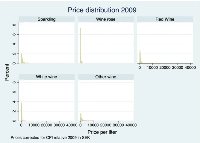
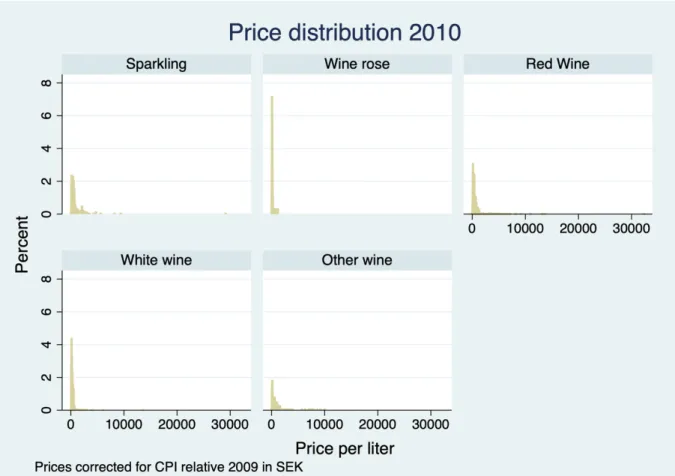
Since the price of wine in the study varies from year to year and also across the varieties. To give an example of the price range figure 3 shows the distribution in 2009 for all five varieties of wine. Distribution curves for all years are found in the appendix. Figure 3 underline the skewness observed in the descriptive statistics.
Figure 3 Distribution of prices in 2009 for all five wine categories
In recent studies observations have been excluded with sales below 10 liters per year (Dahlström & Åsberg, 2009). Other studies have used similar data but only used the
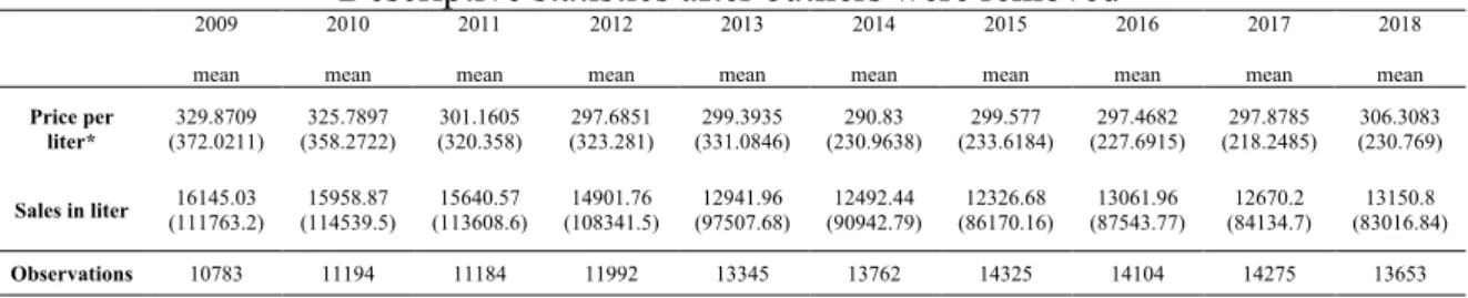
observations with 750 ml bottles (Cuellar et al., 2010). With hopes of removing an as small amount of observations as possible, observations were not removed from the dataset due to the sales nor what kind of bottle the beverages are sold in. This study keeps the observations which are within 2 ∗ 𝜎 from the mean, 95 percent for each commodity detail for each year to control for skewness. Table 2 shows the descriptive statistics after the large outliers were
Descriptive statistics before outliers were removed
2009 2010 2011 2012 2013 2014 2015 2016 2017 2018
mean mean mean mean mean mean mean mean mean mean
Price per
liter* (827.054) 413.7738 (773.9983) 407.1572 (662.3717) 373.213 (924.7472) 388.1784 (898.6481) 382.4316 (753.1491) 378.8557 (773.8938) 393.8945 (723.4539) 392.1017 (718.1912) 397.311 (832.188) 417.3975
Sales in liter 16226.45 (114272) (116189.5) 16199.74 (123063.8) 16459.13 (119242.9) 15625.28 14284.54 (113765) (105977.1) 13777.43 (97888.57) 13189.51 (94765.65) 13496.28 (91768.73) 13338.87 (95335.19) 14214.95 Observations 11182 11599 11608 12451 13855 14358 14980 14764 14961 14326
removed and comparing with table 1, an important change in both mean and standard deviation can be observed. The real price of wine decreased until 2014 when an increase in real prices can be observed until 2018. In figure 4 the distribution of price, the price range is less skewed.
Descriptive statistics after outliers were removed
2009 2010 2011 2012 2013 2014 2015 2016 2017 2018
mean mean mean mean mean mean mean mean mean mean
Price per
liter* (372.0211) 329.8709 (358.2722) 325.7897 (320.358) 301.1605 (323.281) 297.6851 (331.0846) 299.3935 (230.9638) 290.83 (233.6184) 299.577 (227.6915) 297.4682 (218.2485) 297.8785 (230.769) 306.3083
Sales in liter (111763.2) 16145.03 (114539.5) 15958.87 (113608.6) 15640.57 (108341.5) 14901.76 (97507.68) 12941.96 (90942.79) 12492.44 (86170.16) 12326.68 (87543.77) 13061.96 (84134.7) 12670.2 (83016.84) 13150.8 Observations 10783 11194 11184 11992 13345 13762 14325 14104 14275 13653
Standard deviation in parentheses. *Corrected for CPI Table 2 Descriptive statistics after outliers were removed
4.1.1 Creating an agregated data set
This study assume that wine is a differentiated good, however it is difficult to differentiate over each observation of wine, why the total sales were used to estimate the demand for wine. The dataset was aggregated over each wine category per year and a pooled dataset of 50 observations was created. With the total sales and simple average price and a weighted arithmetic mean which was calculated before the dataset was aggregated:
𝑠( =…_†_
a‡ (17) 𝑅ˆ = 𝑝f𝑞f+ ⋯ + 𝑝Z𝑞Z
𝑖 = Observation of the unique product
𝑐 = Variety, Sparkling, Rose, Red, White or Other wine 𝑠( = Budget share
∑Z)D(ln(𝑝() ∗ 𝑠( = ln (pR∗) (18)
The aggregated data set is strongly balanced, since no observations are missing. The new dataset consists out of 5 groups and observations for 10 years, the number of observations is therefore 50.
4.2 Limitations
The data does not contain the degree of alcohol, and the levels of ethanol can therefore not be accounted for. Since the degree of ethanol is not provided in the dataset, the impact of tax changes to the demand for alcohol is not estimated. Due to the annual data, this study cannot control for differences in consumption patterns throughout the year.
This study uses sales data and not households or per capita consumption, the socio-economic perspective is not taken into account in the price elasticities estimates which have been raised as a problem when estimating price elasticities (Babor et al., 2010). However, this is
suggested for further studies on the demand elasticities of Wine and alcohol in Sweden as supposed by Green & Alston (1990). No controls for regional differences in consumption will be accounted for since the dataset correspond only to the national sales of alcohol.
5 Analysis and discussion
In this chapter the results from the Single equation model will be discussed first followed by the results from the L/AIDS model to be concluded with a brief comparison between the results from the two models.
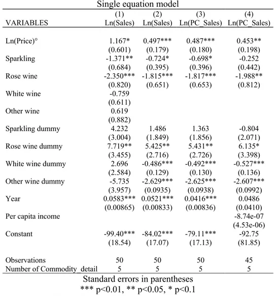
5.1 Single equation model
In total five models were estimated, in the first estimation it can be observed that the
estimates for White and Other wine are not significant when included in the model. If the two categories are included in the intercept together with Red wine, as can be observed in the second regression. The own price elasticity for Sparkling is -1.227, for Rose wine -2.318 and the own price elasticity for the unobserved values, Red, White and other wine is -0.503. The demand for Sparkling and Rose is elastic since the own price elasticities in absolute terms are greater than one and significant at least at the 10 percent level. The clustered demand for Red, White and other is however inelastic and significant at the 1 percent level.
Single equation model
(1) (2) (3) (4)
VARIABLES Ln(Sales) Ln(Sales) Ln(PC_Sales) Ln(PC_Sales)
Ln(Price)° 1.167* 0.497*** 0.487*** 0.453** (0.601) (0.179) (0.180) (0.198) Sparkling -1.371** -0.724* -0.698* -0.252 (0.684) (0.395) (0.396) (0.442) Rose wine -2.350*** -1.815*** -1.817*** -1.988** (0.820) (0.651) (0.653) (0.812) White wine -0.759 (0.611) Other wine 0.619 (0.882) Sparkling dummy 4.232 1.486 1.363 -0.804 (3.004) (1.849) (1.856) (2.071)
Rose wine dummy 7.719** 5.425** 5.431** 6.135*
(3.455) (2.716) (2.726) (3.398)
White wine dummy 2.696 -0.486*** -0.492*** -0.527***
(2.584) (0.129) (0.130) (0.136)
Other wine dummy -5.735 -2.629*** -2.625*** -2.607***
(3.957) (0.0935) (0.0938) (0.0992)
Year 0.0583*** 0.0521*** 0.0416*** 0.0486
(0.00865) (0.00833) (0.00836) (0.0410)
Per capita income -8.74e-07
(4.53e-06)
Constant -99.40*** -84.02*** -79.11*** -92.75
(18.54) (17.07) (17.13) (81.85)
Observations 50 50 50 45
Number of Commodity_detail 5 5 5 5
Standard errors in parentheses *** p<0.01, ** p<0.05, * p<0.1
°Controlled for CPI, weighted arithmetic mean
Table 3 Single equation model
In regression 3-4 the Per capita sales are estimated. The outcome variable is therefore total per capita sales in natural log. The estimates do not vary a lot comparing to regression 1 and 2. The own price elasticity for Sparkling is --1,211, for Rose wine -2.33 and the own price elasticity for the reference group, Red, White and other wine is -0.513. The time effects seams
to capture the change in per capita income, since when adding the control variables Per capita income, none of the control variables are significant and however the estimated elasticity for Rose and the clustered elasticity show a marginal change, however, Sparkling becomes insignificant.
5.2 LAIDS
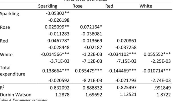
The Durbin Watson test for the Sparkling and Red are close but still not close enough in order to reject the autocorrelation. The Durbin Watson for Rose and White are relatively close to 2 and autocorrelation can therefore be rejected. The adding up constraint is tested and satisfied, homogeneity is also tested and rejected for all except for Other, were homogeneity cannot be rejected. The R2 are relatively close to zero and indicates a somewhat fit model, even though,
one should not put too much weight into the R2.
Parameter estimates
Sparkling Rose Red White
Sparkling -0.05302** -0.026198 Rose 0.025099** 0.072164* -0.011283 -0.038081 Red 0.046778* -0.013669 0.020861 -0.028448 -0.02187 -0.037258 White -0.014566*** -1.22E-03 -0.034102*** 0.055552*** -3.71E-03 -7.12E-03 -7.15E-03 -2.25E-03 Total
expenditure 0.138664*** 0.055479*** -0.144469*** -0.010714*** -0.020592 -8.21E-03 -0.021793 -2.74E-03
R2 0.832092 0.888832 0.825497 .991849
Durbin Watson 1.2878 1.69692 1.12521 1.8722
Table 4 Parameter estimates
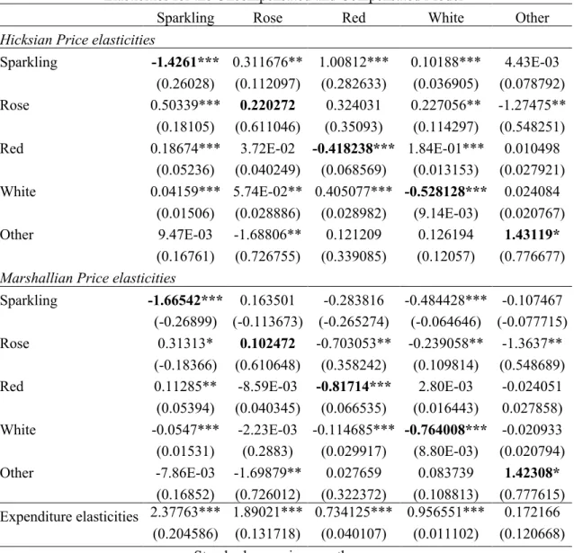
The Marshallian own price elasticities in Table 5 are negative and significant at the one percent level for Sparkling, Red and White. But positive for Rose respectively Other wine and statistically insignificant and significant at the 10 percent level respectively, Since all the Marshallian own price elasticities in, does not have negative estimates, we can conclude that this does not satisfy consumer theory (Edgerton et al., 1996). Reasons for this might be that the number of observations is fairly low and might lead to ambiguous results.
Elasticities for the Uncompensated and Compensated Model
Sparkling Rose Red White Other
Hicksian Price elasticities
Sparkling -1.4261*** 0.311676** 1.00812*** 0.10188*** 4.43E-03
(0.26028) (0.112097) (0.282633) (0.036905) (0.078792)
Rose 0.50339*** 0.220272 0.324031 0.227056** -1.27475**
(0.18105) (0.611046) (0.35093) (0.114297) (0.548251)
Red 0.18674*** 3.72E-02 -0.418238*** 1.84E-01*** 0.010498
(0.05236) (0.040249) (0.068569) (0.013153) (0.027921)
White 0.04159*** 5.74E-02** 0.405077*** -0.528128*** 0.024084
(0.01506) (0.028886) (0.028982) (9.14E-03) (0.020767)
Other 9.47E-03 -1.68806** 0.121209 0.126194 1.43119*
(0.16761) (0.726755) (0.339085) (0.12057) (0.776677)
Marshallian Price elasticities
Sparkling -1.66542*** 0.163501 -0.283816 -0.484428*** -0.107467
(-0.26899) (-0.113673) (-0.265274) (-0.064646) (-0.077715)
Rose 0.31313* 0.102472 -0.703053** -0.239058** -1.3637**
(-0.18366) (0.610648) (0.358242) (0.109814) (0.548689)
Red 0.11285** -8.59E-03 -0.81714*** 2.80E-03 -0.024051
(0.05394) (0.040345) (0.066535) (0.016443) 0.027858) White -0.0547*** -2.23E-03 -0.114685*** -0.764008*** -0.020933 (0.01531) (0.2883) (0.029917) (8.80E-03) (0.020794) Other -7.86E-03 -1.69879** 0.027659 0.083739 1.42308* (0.16852) (0.726012) (0.322372) (0.108813) (0.777615) Expenditure elasticities 2.37763*** 1.89021*** 0.734125*** 0.956551*** 0.172166 (0.204586) (0.131718) (0.040107) (0.011102) (0.120668) Standard errors in parentheses
*** p<0.01, ** p<0.05, * p<0.1
Table 5 AIDS - Price elasticities
In table 5, representing the Uncompensated and Compensated model, the elasticities are calculated from budget share, which means that the elasticities does not imply that an increase in disposable income would increase the spending in quantity but increasing the budget share, as well as an increase in price is not associated with a decrease in quantity but a potential decrease in budget share. The demand for Sparkling is elastic since the estimate is greater than one in absolute terms. The demand for Red and White is price inelastic, meaning that consumers of Red and White wine are less responsive to price changes.
For the Compensated elasticities, the own price elasticities are lower for the significant values than in the Uncompensated elasticities which is expected since the uncompensated elasticities result in more elastic estimates (Fogarty, 2009). The own-price elasticity estimates have the same elasticity as in the uncompensated estimates.
For the cross-price elasticities however, the elasticities have a higher degree of statistically significant estimates. For Sparkling, Rose and White are net substitutes, and Red wine net complement differing from the Uncompensated model. For Rose, White is a net supplement
compared to the Uncompensated, where it is considered a compliment. For Red, Sparkling and White are net substitutes. For White, Sparkling, Rose and Red are considered net substitutes ranging from 5.74E-02 to 0.405077, except Other which is not statistically significant. Rose is a net complement for Other. When estimating the Hicksian demand, the utility is kept constant, the estimates represents the mean elasticities for the different varieties of the Swedish consumer.
Concerning the cross-price elasticities in the Uncompensated model, only a few of them are statistically significant. For Sparkling, the estimate implies that White wine is a gross complement. For Rose, Sparkling is a gross substitute whereas Red, White and Other are gross complements. For Red, Sparkling is a gross substitute. For White, Sparkling and Red are gross complements. For Other, Rose is a gross complement. For the remaining estimates, were not statistically significant why no assumption regarding potential substitution or complementary effects can be made.
The expenditure elasticities are all statistically significant, except for Other, the estimated elasticities for Sparkling and Rose, are greater than one indicating that both are luxury goods. Red is well below one, indicating that Red is a necessary good. The expenditure elasticity for White is very close to one indicating that it is very close to be considered a luxury good, however, it still falls into the category of a necessary good. The expenditure elasticities resembles the results shown by Carew et al. (2004) where White wine has a higher elasticity than Red wine. Dahlström & Åsberg (2009) argues that this is a result of shifts in the food consumption, since swedes tend to eat more shellfish and fish when income increases which may coincide with the consumption of White wine.
The results for the estimates for own-price elasticities are not consistent over the two models, in the Single equation model, the demand for White, Rose and Sparkling are elastic whereas in the L/AIDS model, the demand for Rose and White are inelastic. L/AIDS have the imposed adding up, symmetry and homogeneity restrictions, not imposed in the Single equation model. The differences in the accuracy in the models have been discussed and argued that the Single equation model may lead to ambiguous results (Fogarty, 2009). By providing both results in this study capture that wine is a heterogenous good even at a color level, why a system approach is necessary to account for consumer demand.
6 Conclusions
Over the time period studied, the numbers of choice for wine for the Swedish consumer have increased as well as the levels of total sales of wine. Using the system demand approach this study have shed light over the own price elasticities and cross price elasticities within wine. The results suggest that Sparkling and Rose are luxury goods, whereas red is a necessity and White wine is in an ambivalent zone between luxury and necessity. Concerning the cross-price elasticities, the compensated and uncompensated estimates varied quite substantially, which may depend on lack of observations or the limitation of time. The demand for Red and White wine is inelastic which implies that consumers are not sensitive regarding changes in price whereas the demand for Sparkling is elastic and is more sensitive to price changes. To decrease the consumption in order to achieve the WHO goals for 2025 it might be interesting to look further into the elasticities of demand across varieties in order to go about the
substitution effects. Since sensibility in prices may affect policy outcome, in order to estimate potential tax implications, accessibility for the ethanol data is required for further studies. The two approaches toward the demand of wine shows that a Single equation model does not manage to capture the differences within the varieties of wine, why a system demand, is more relevant to apply to such a heterogeneous good. However, including more control variables such as organic, vintage and quality factors using ethanol levels, would acquire a more in depth understanding of the wine market in Sweden.
The quality of data for similar demand estimations have been discussed and in order to analyze the demand for wine as well as other alcoholic beverages in comparison with other food stuff, the data needs to be more detailed and collectable in the same place. Which would open up for more analysis regarding consumption patterns and taxation.
References
Afifi, A. A., Kotlerman, J. B., Ettner, S. L., & Cowan, M. (2007). Methods for Improving Regression Analysis for Skewed Continuous or Counted Responses. Annual Review of
Public Health, 28(1), 95–111.
https://doi.org/10.1146/annurev.publhealth.28.082206.094100
Alley, A. G., Ferguson, D. G., & Stewart, K. G. (1992). An almost ideal demand system for alcoholic beverages in British Columbia. Empirical Economics, 17(3), 401–418. https://doi.org/10.1007/BF01206301
Alston, J. M., Foster, K. A., & Gree, R. D. (1994). Estimating Elasticities with the Linear Approximate Almost Ideal Demand System: Some Monte Carlo Results. The Review
of Economics and Statistics, 76(2), 351. https://doi.org/10.2307/2109891
Asplund, M., Friberg, R., & Wilander, F. (2007). Demand and distance: Evidence on cross-border shopping. Journal of Public Economics, 91(1–2), 141–157.
https://doi.org/10.1016/j.jpubeco.2006.05.006
Babor, T. F., Caetano, R., Casswell, S., Edwards, G., Giesbrecht, N., Graham, K., … Rossow, I. (2010). Alcohol: No Ordinary Commodity.
https://doi.org/10.1093/acprof:oso/9780199551149.001.0001
Barnett, W. A., & Seck, O. (2008). Rotterdam model versus almost ideal demand system: will the best specification please stand up? Journal of Applied Econometrics, 23(6), 795– 824. https://doi.org/10.1002/jae.1009
Barten, A. P. (1964). Consumer demand functions under conditions of almost additive preferences. Econometrica, 32, 1–38.
Carew, R., Florkowski, W. J., & He, S. (2004). Demand for Domestic and Imported Table Wine in British Columbia: A Source-differentiated Almost Ideal Demand System Approach. Canadian Journal of Agricultural Economics/Revue Canadienne
D'Agroeconomie, 52(2), 183–199.
https://doi.org/10.1111/j.1744-7976.2004.tb00101.x
Clements, K. W., & Gao, G. (2015). The Rotterdam demand model half a century on.
Economic Modelling, 49, 91–103. https://doi.org/10.1016/j.econmod.2015.03.019
Cook, P. J., & Moore, M. J. (2000). Alcohol (1st ed; A. J. Culyer & J. P. Newhouse, Eds.). Amsterdam ; New York: Elsevier.
Cuellar, S. S., Colgan, T., Hunnicutt, H., & Ransom, G. (2010). The demand for wine in the USA. International Journal of Wine Business Research, 22(2), 178–190.
https://doi.org/10.1108/17511061011061739
Cuellar, S. S., & Huffman, R. (2008). Estimating the Demand for Wine Using Instrumental Variable Techniques. Journal of Wine Economics, 3(2), 172–184.
https://doi.org/10.1017/S193143610000119X
Dahlström, T., & Åsberg, E. (2009). Determinants of Demand for Wine – price sensitivity and perceived quality in a monopoly setting. CESIS Electronic Working Paper Series, 182, 40.
Dameus, A., Richter, F. G.-C., Brorsen, B. W., & Sukhdial, K. P. (2002). AIDS versus the Rotterdam demand system: a Cox test with parametric bootstrap. Journal of
Davis, T. R., Ahmadi-Esfahani, F. Z., & Iranzo, S. (2008). Demand under product
differentiation: an empirical analysis of the US wine market*. Australian Journal of
Agricultural and Resource Economics, 52(4), 401–417.
https://doi.org/10.1111/j.1467-8489.2008.00419.x
Deaton, A., & Meullbauer, J. (1980). An Almost Ideal Demand System. The American
Economic Review, 70(3), 312–326.
Duffy, M. H. (1987). Advertising and the inter-product distribution of demand. European
Economic Review, 31(5), 1051–1070. https://doi.org/10.1016/S0014-2921(87)80004-1
Edgerton, D. L., Assarsson, B., Hummelmose, A., Laurila, I. P., Rickertsen, K., & Vale, P. H. (1996). The Econometrics of Demand Systems. https://doi.org/10.1007/978-1-4613-1277-2
Fogarty, J. (2006). The nature of the demand for alcohol: understanding elasticity. British
Food Journal, 108(4), 316–332. https://doi.org/10.1108/00070700610657155
Fogarty, J. (2009). THE DEMAND FOR BEER, WINE AND SPIRITS: A SURVEY OF THE LITERATURE. Journal of Economic Surveys. https://doi.org/10.1111/j.1467-6419.2009.00591.x
Friberg, R., & Grönqvist, E. (2012). Do Expert Reviews Affect the Demand for Wine?
American Economic Journal: Applied Economics, 4(1), 193–211.
https://doi.org/10.1257/app.4.1.193
Green, R., & Alston, J. M. (1990). Elasticities in AIDS Models. American Journal of
Agricultural Economics, 72(2), 442. https://doi.org/10.2307/1242346
Gruenewald, P. J., Ponicki, W. R., Holder, H. D., & Romelsjo, A. (2006). Alcohol Prices, Beverage Quality, and the Demand for Alcohol: Quality Substitutions and Price Elasticities. Alcoholism: Clinical and Experimental Research, 30(1), 96–105. https://doi.org/10.1111/j.1530-0277.2006.00011.x
Gujarati, D. N. (2003). Basic econometrics (4th ed). Boston: McGraw Hill.
Lööv, H., & Widell, L. M. (2009). Konsumtionsförändringar vid ändrade matpriser och
inkomster (No. 2009:8).
Mitchell, L. (2016). Demand for Wine and Alcoholic Beverages in the European Union: A Monolithic Market? Journal of Wine Economics, 11(3), 414–435.
https://doi.org/10.1017/jwe.2016.17
Regeringskansliet. (2018, June 29). Regeringen vill se permanent hemkörning från Systembolaget [Text]. Retrieved May 10, 2019, from Regeringskansliet website: https://www.regeringen.se/pressmeddelanden/2018/06/regeringen-vill-se-permanent-hemkorning-fran-systembolaget/
Room, R. (2004). Att lappa ihop en politikstudie. Nordic Studies on Alcohol and Drugs,
21(4–5), 345–349. https://doi.org/10.1177/1455072504021004-501
SCB. (2019a, January 14). Priserna i Sverige – Konsumentprisindex (KPI). Retrieved May 2, 2019, from Statistiska Centralbyrån website: http://www.scb.se/hitta-statistik/sverige-i-siffror/samhallets-ekonomi/kpi/
SCB. (2019b, April 29). Inkomster och skatter. Retrieved May 18, 2019, from Statistiska Centralbyrån website: http://www.scb.se/hitta-statistik/statistik-efter-amne/hushallens-ekonomi/inkomster-och-inkomstfordelning/inkomster-och-skatter/
Selvanathan, E. A. (1991). Cross-country alcohol consumption comparison: an application of the Rotterdam demand system. Applied Economics, 23(10), 1613–1622.
https://doi.org/10.1080/00036849100000126
Selvanathan, S., & Selvanathan, E. A. (2005). Empirical Regularities in Cross-Country Alcohol Consumption*. Economic Record, 81(s1), S128–S142.
https://doi.org/10.1111/j.1475-4932.2005.00250.x
Skatteverket. (n.d.). Skattesatser på alkohol [Tax agency]. Retrieved February 21, 2019, from Skatteverket.se website:
https://www.skatteverket.se/foretagochorganisationer/skatter/punktskatter/alkoholskatt /skattesatser.4.4a47257e143e26725aecb5.html
Stock, J. H., & Watson, M. W. (2015). Introduction to econometrics (Updated third edition, global edition). Boston Columbus Indianapolis New York San Francisco Hoboken Amsterdam Cape Town Dubai London: Pearson.
Sundén, D. (2019). Synd och skatt. ESO-rapport 2019: En ESO-rapport om politiken inom
områdena alkohol, tobak och spel. Norstedts Juridik AB.
Systembolaget. (2018). Systembolaget’s Responsibility Report 2017 (p. 128) [Statistiska meddelanden]. Retrieved from https://www.omsystembolaget.se/globalassets/pdf/om-systembolaget/responsibility-report-2017.pdf
Systembolaget. (n.d.-a). Försäljningsstatistik. Retrieved January 26, 2019, from omsystembolaget.se website: https://www.omsystembolaget.se/om-systembolaget/foretagsfakta/forsaljningsstatistik/
Systembolaget. (n.d.-b). Från bergsmän till Bratt. Retrieved February 20, 2019, from http://www.systembolagethistoria.se/teman/ursprunget/
Systembolaget. (n.d.-c). Om vår organisation | Systembolaget. Retrieved May 10, 2019, from /om-systembolaget/foretagsfakta/organisation2/
Systembolaget. (n.d.-d). ”Operation vin”. Retrieved January 26, 2019, from http://www.systembolagethistoria.se/teman/kampanjer/operation-vin/
Systembolaget. (n.d.-e). Vi säljer alkohol med ansvar | Systembolaget. Retrieved May 11, 2019, from /vart-uppdrag/salja-med-ansvar/
Systembolaget. (n.d.-f). Viktiga vändpunkter. Retrieved May 24, 2019, from http://www.systembolagethistoria.se/teman/handelser/
Theil, H. (1965). The information approach to demand analysis. Econometrica, (33), 67–87. Trolldal, B., & Leifman, H. (2018). Alkoholkonsumtionen i Sverige 2017 (No. 175; p. 54).
Retrieved from CAN website:
https://www.can.se/contentassets/00aedc7994c94a34b2f35880ba8e1083/alkoholkonsu mtionen-i-sverige-2017_webb.pdf
Varian, H. R. (2010). Intermediate microeconomics: a modern approach (8. ed). New York, NY: Norton.
World Health Organization, & Management of Substance Abuse Team. (2018). Global status
report on alcohol and health 2018. Retrieved from
Appendix
Figure 6 Price distribution 2011
Figure 10 Price distribution 2015
Figure 12 Price distribution 2017
Figure 14 Price distribution 2010 - Corrected for skewness
Figure 16 Price distribution 2012 - Corrected for skewnes
Figure 18 Price distribution 2014 - Corrected for skewness
Figure 20 Price distribution 2016 - Corrected for skewness
Figure 22 Price distribution 2018 - Corrected for skewness
Fixed effect
VARIABLES Sparkling Rose Red White Other LN(Simple mean price)° (0.338) (4.511) (0.189) 0.323 -5.132 -0.147 1.522** (0.634) (0.192) 0.389* Year 0.128*** 0.254 0.0148*** 0.00228 -0.0110*** (0.00900) (0.139) (0.00213) (0.0109) (0.00310) Constant -238.0*** -465.3 -6.121 9.335 40.33*** (19.85) (257.6) (4.713) (19.36) (6.793) Observations 10 10 10 10 10 R-squared 0.988 0.910 0.890 0.715 0.801 Standard errors in parentheses
*** p<0.01, ** p<0.05, * p<0.1 °Controlled for CPI