Modelling and simulation of heat conduction in 1-D polar spherical coordinates using control volume-based finite difference method

http://www.diva-portal.org

Postprint

This is the accepted version of a paper published in International journal of numerical methods for heat & fluid flow. This paper has been peer-reviewed but does not include the final publisher proof-corrections or journal pagination.

Citation for the original published paper (version of record): Diószegi, A., Diószegi, E., Tóth, J., Svidró, J T. (2016)

Modelling and simulation of heat conduction in 1-D polar spherical coordinates using control volume-based finite difference method.

International journal of numerical methods for heat & fluid flow, 26(1): 2-17 http://dx.doi.org/10.1108/HFF-10-2014-0318

Access to the published version may require subscription. N.B. When citing this work, cite the original published paper.

Permanent link to this version:

Modelling and simulation of heat conduction in 1-D

polar spherical coordinates using control

volume-based finite difference method

Attila Diószegi

Jönköping University School of Engineering, Department of Materials and Manufacturing -

Foundry Technology, Jönköping, Sweden

Éva Diószegi

Diocore AB, Jönköping, Sweden

Judit Tóth

University of Miskolc, Department of Foundry Technology, Miskolc, Hungary

József Tamás Svidró

Jönköping University School of Engineering, Department of Materials and Manufacturing -

Foundry Technology, Jönköping, Sweden

Abstract

Purpose - The purpose of this paper to obtain a finite difference method (FDM) solution using control volume

for heat transport by conduction and the heat absorption by the enthalpy model in the sand mixture used in casting manufacturing processes. A mixture of sand and different chemicals (binders) is used as moulding materials in the casting processes. The presence of various compounds in the system improve the complexity of the heat transport due to the heat absorption as the binders are decomposing and transformed into gaseous products due to significant heat shock.

Design/methodology/approach - The geometrical domain were defined in a 1D polar coordinate system and

adapted for numerical simulation according to the control volume based finite difference method (CV-FDM). The simulation results were validated by comparison to the temperature measurements under laboratory conditions as the sand mould mixture was heated by interacting with a liquid alloy.

Findings - Results of validation and simulation methods were about high correspondence, the numerical method

presented in this paper is accurate and has significant potential in the simulation of casting processes.

Originality/value - Both numerical solution (definition of geometrical domain in 1D polar coordinate system)

and verification method presented in this paper are state-of-the-art in their kinds and present high scientific value especially regarding to the topic of numerical modelling of heat flow and foundry technology.

Keywords Casting, heat absorption, heat conduction, modelling, moulding materials, polar spherical

coordinates, thermal analysis, CV-FDM.

Nomenclature Small letters: p c Specific heat, Jkg-1_K-1 * p

c Relative heat capacity, Jkg-1K-1

V

c

Volumetric heat capacity, Jm-3_K-1

a

f Volume fraction of transformed phase

k Thermal conductivity, Wm-1_K-1

cond

q

Diffusive heat flow perpendicular through the surface of the area, W

r

Spatial parameters for spherical coordinate systems, m

x

Descriptive space parameter perpendicular to the surface, m

2 1

, x

x

Wall-surface positions, m x ∆ Wall thickness, m t ∆ Time difference, s Capital letters:

A Area of the surface, through which the heat flow takes place, m2

L Heat required for binder decomposition, Jkg-1

i i

M

_−1→ Heat resistance coefficient between nodes i-1 and I,

1 + →i

i

M

Heat resistance coefficient between nodes i and i+1

gen

Q Released heat during solidification, Wm-3

abs

Q

Heat absorbed by moulding material, Wm-3

R

R_thcond, Heat conduction resistance, m2_KW-1

T Temperature, °C 2 1

,T

T

Wall-surface temperatures, °C T ∆ Temperature difference, °C V Volume, m3 Greek symbols: ρ Density, kgm-3

Θ Linear combination parameter

T

2

∇

Laplace operator, °Cm-2

1. Introduction

Using of moulding materials (moulds and cores) are essential in the majority of casting manufacturing processes. Internal channels and complex geometries are formed by the placement of sand cores within the mould cavity. These cores consist of refractory materials (different types of sands) and organic or inorganic binders.

Sand cores suffer significant heat shock as interacting with liquid metal due to high heating rates, various gases evolve from the moulding material as a result of binder decomposition. Thermo physical properties of moulding materials such as heat capacity influence the solidification process, the microstructure of casting and the formation of different casting defects. The thermo physical properties of sand cores are depend on the binder content, the type of binder, the type of used sand, etc.

Hence, the moulding material related heat transfer processes are considerably complex, databases and models regarding to this phenomena are underdeveloped even in the state-of-the-art casting simulation software products. Thus, much detailed understanding and more accurate modelling methods are required to develop the casting production process.

Modelling and simulation of casting processes are widely spread in foundry research, including models for simulating solidification of liquid metals, microstructure formation, mechanical properties, stresses and strains in castings. (Svensson and Diószegi, 2000) (Bhattacharya and Dutta, 2013) (Svensson and Dugic, 1999) (Ransing et al., 1999) (Cruchaga et al., 2004) (Lewis et al., 2004) (Lee et al., 2004) (Nastac and Stefanescu, 1997) (Ramirez and Beckermann, 2005) (Chang and Dantzig, 2004)

Heat transfer processes taking place inside sand moulds and cores are considerably complex, related models and databases are less developed then for phenomenon related to the cast metal. For this reason, a detailed understanding and accurate modelling is required to investigate the “sand side” of the entire casting production circle.

In previous works (Winardi et al., 2007) (Krajewski et al., 2014) efforts have been dedicated to improve the understanding of the heat transfer in sand moulds including the investigation of heat absorption due to the gas binder decomposition. An experimental method presented by the authors (Svidró et al., 2014) include spherical shaped sand core samples to be immersed in the liquid metal for investigating the thermal properties of the sand mixtures. A well-known numerical procedure from the literature (Hattel, 2005) is the FDM-CV method which have been found described only for Cartesian and polar cylindrical coordinates. The scope of the present work is to adapt the FDM-CV method to polar spherical coordinates thereby allowing the comparison between measured and calculated temperature changes in spherical shaped sand core samples.

1.1 Basic types of heat transfer in moulding materials

Heat transfer in granular moulding materials proceed in three separate ways: by conduction, convection and radiation. Thermo physical properties are relatively difficult to describe in sand cores because of appearance of all basic types of heat transfer methods in one time, and the presence of chemical reactions resulting in material transports due to the heat introduced by the molten metal.

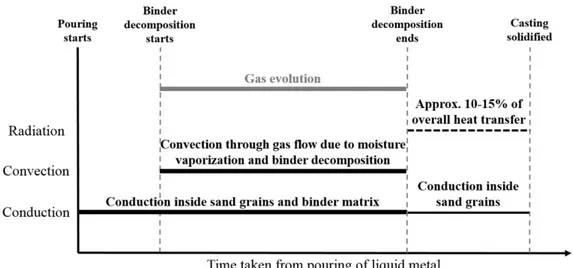
Figure 1 shows the schematics of heat transport modes inside a sand core versus time taken from the beginning of the mould filling.

Figure 1. Basic heat transfer methods inside a sand core during metal casting process.

Conduction is the most significant type of heat transport inside moulds and sand cores, which takes place inside the sand grains through the entire casting production from the mould filling process until the solidification of the casting. Furthermore heat is transported also by conduction inside binder matrices keeping the sand grains together. This phenomenon plays a part in until the complete decomposition of binder matrices inside the core.

Inside sand cores, heat can be transported by forced convection due to the vaporization of free moisture and bonded water content, and decomposition of the binders resulting in gas evolution. The thermo physical properties of overheated steam and different organic gases are similar to the properties of air. As far as gas flow is present in the system (during the binder decomposition process), forced convection affects the effective heat transport inside the moulding materials. This phenomenon can be actually considered as energy transport driven material transport.

Heat is transported by radiation between non-contacted sand grains after the decomposition of the binder matrices and depends on pore size and temperature. In case of lower temperatures, radiation can be neglected up until 900°C due to the small pore size in moulding materials. Above 900°C the rate of radiation is increasing and subjects about 10-15% of the overall effective heat transport. However, this

has slight effect from foundry technology point of view because the cast part has already solidified until the temperature in sand cores reach high rates. Before binder decomposition, casting skin should usually form.

In this work only heat conduction is modelled and simulated, thus discussed in general in the next chapter.

1.2. Heat conduction

When a temperature gradient exists in a body, experience has shown that there is an energy transfer from the high temperature region to the low temperature region. In this case, it is said that the energy is transferred by conduction. The heat flow per unit area is proportional to the normal temperature gradient, where the proportionality constant is the thermal conductivity

x T kA q ∂ ∂ − = cond (1)

Equation 1 is called Fourier’s law of heat conduction and it should be noted that it is the defining equation for thermal conductivity (k).

Term of thermal resistance is important to define considering heat conduction. For this purpose a plane wall is considered. If steady-state conditions are assumed, i.e. no time dependence, that is T=T(x) only, Fourier’s law can be integrated as

∫

=−

∫

→ ∂ ∂ − = 2 1 2 1 d d cond x x T T T k x A q x T kA q (2)

Where x1, x2 and T1, T2 are wall-surface positions and temperatures, respectively. Equation 2 is often

referred as Fourier’s law on integral form. Assuming a constant thermal conductivity, k, the integration now yields

(

2 1

)

1 2 cond T T x x kA q − − − = (3)

Rearranging in terms of wall thickness ∆x and temperature difference ∆T gives

kA

x

R

R

T

q

=

−

∆

→

_thcond

=

∆

cond th cond (4)

Based on this equation a different conceptual viewpoint is introduced for Fourier’s law. The heat transfer rate is considered as a flow, and the combination of thermal conductivity, thickness of material and area as resistance to this flow. The temperature is the potential or driving parameter for the heat flow. This way Equation 4 can be interpreted as

resistance conductive Thermal difference potential Thermal cond =− q (5)

The concept of thermal resistance is very useful when analysing the solidification of real 3-D castings, although being based on 1-D steady-state assumptions. This holds for the derivation of analytical solutions as well as formulation of numerical methods. (Hattel, 2005)

2. Theory for heat distribution in sand cores

2.1 Analytical definition of Fourier’s law of heat conduction in spherical coordinates

Figure 2 shows arbitrary control volume in a spherical system with radius r as the only space parameter. Three nodes are considered as sphere layers, i-1, i and i+1. Distance from the centre out to the point i in the control volume is termed r.

Figure 2. Mesh in the 1-D spherical formulation.

Area of sphere inserted to Equation 1

2 4 r A x T kA q → = π ∂ ∂ − = (6) Gives T k r r q d d 4π 2 =− (7)

Which, integrated yields

∫

∫

− =− 2 1 2 1 d d 4 2 T T r r T k r r q

π

(8)

(

_{2 1}

)

1 2 1 1 4 k T T r q r r − − =         − − π (9)

(

)

(

2 1

)

1 1 1 2 4 r r k T T q − ₋ − _{=− −} π (10)

Equation 10 expressed to q gives

(

)

(

)

2 1 2 1 1 2 1 2 1 1 4 1 1 4 r r T T k q r r T T k q − − = → − − =

π

π

(11)

the analytical definition of the heat conduction in spherical coordinates.

2.2 Numerical definition of Fourier’s law of heat conduction in spherical coordinates

Heat balance was written for a control volume by earlier author (Hattel, 2005) in the process of creating mathematical models for calculating latent heat released during casting solidification: Change of heat content pr. time unit = Sum of heat fluxes into the volume over N surfaces + Released heat during solidification.

∑

= + ₊ − = N j j j _{q Q} Q 1 gen 1 ) 1 ( (12)

where overall heat content of the system is given by t T c V Q _p ∂ ∂ = ρ (13)

The heat fluxes are expressed by means of thermal resistances (Equation 4). From the centre of node i-1 to the centre of node i yields

i i i i i i R T T q → − − → − =− − 1 1 1 (14)

and from the centre of node i to the centre of node i+1 yields

1 1 1 + → + + → =− − i i i i i i R T T q (15)

In case of sand cores “+” in Equation 12 should be change to “-“, thus heat absorption processes are considered besides latent heat released during solidification. Therefore the correct form of Equation 12 for heat absorption is given by

∑

= + ₋ − = N j j j Q q Q 1 abs 1 ) 1 ( (16)

Inserting Equation 13 together with Equation 14 and Equation 15 into Equation 16, yields

( )

i i i i i i i i i i i i i i i i p i Q R T T R T T Q q q t T c V _abs, 1 1 1 1 abs, 1 1 −     ₋ − − − − = − − = ∂ ∂ + → + → − − + → → −

ρ

(17)

Equation 17 rearranged gives the numerical definition of heat conduction in spherical coordinates

( )

i i i i i i i i i i i p i Q R T T R T T t T c V abs, 1 1 1 1− ₊ − ₋ = ∂ ∂ + → + → − − ρ (18)

2.3 Numerical definition of heat resistance and spherical geometry

On the basis of Equation 11, thermal resistance in spherical coordinates is given by

k r r R π 4 1 1 2 1 cond th − = (19)

Thermal resistance is changing inside the nodes, so it is necessary to define it from the centre of node i-1 to the centre of node i:

k r r r R i i i i _π 4 1 2 1 left − ∆ − = (20)

k r r r R i i i i _π 4 2 1 1 right ∆ + − = (21)

Thermal resistance from the centre of node i-1 to the centre of node i, now yields

interface 1 left right 1 1 i i i i i i R R R R_−→ = ₋ + + _−→ (22) 1 1 1 1 right 1 4 2 1 1 − − − − − ∆ + − = i i i i i k r r r R π (23) i i i i i k r r r R π 4 1 2 1 left − ∆ − = (24) 2 1 interface 1 2 4       ₋∆ = −→ → − i i i i i i r r M R π (25) 2 1 1 1 1 1 1 2 4 4 1 2 1 4 2 1 1       ₋∆ + − ∆ − + ∆ + − = −→ − − − − → − i i i i i i i i i i i i i i r r M k r r r k r r r R

π

π

π

(26)

Thermal resistance from the centre of node i to the centre of node i+1 yields

interface 1 left 1 right 1 + →+ + →i = i + i + i i i R R R R (27) i i i i i k r r r R π 4 2 1 1 right ∆ + − = (28) 1 1 1 1 left 1 4 1 2 1 + + + + + − ∆ − = i i i i i k r r r R π (29) 2 1 1 1 interface 1 2 4       ₋∆ = + + + → + → i i i i i i r r M R π (30)

2 1 1 1 1 1 1 1 1 2 4 4 1 2 1 4 2 1 1       ₋∆ + − ∆ − + ∆ + − = + + + → + + + + + → i i i i i i i i i i i i i i r r M k r r r k r r r R

π

π

π

(31)

The volume of sphere based on nodes is written as:

3 3 3 2 3 4 2 3 4 3 4       ₋∆ −       ₊∆ = = i i i i r r r r r V π π π (32)               ∆ +       ∆ + ∆ + = 3 2 2 3 2 2 3 2 3 3 4 i i i i i i r r r r r r V

π

(33)               ∆ −       ∆ + ∆ − − = 3 2 2 3 2 2 3 2 3 3 4 i i i i i i r r r r r r V

π

(34) 3 2 2 2 3 4 2 6 3 4       ∆ + ∆ = i i i r r r V π π (35)               ∆ + ∆ = 3 2 2 2 2 6 3 4 i i i r r r V

π

(36)               ∆ +       ∆ + ∆ = 3 3 2 2 2 3 3 4 i i i i r r r r V

π

(37)         _{∆ +}∆ = 4 3 3 4 2 i3 i i r r r V π (38)         _{∆ +}∆ = 12 4 3 2 i i i r r r V π (39)

2.3 Solution of Fourier’s law of heat conduction in 1-D polar spherical coordinates with control volume based finite difference method

Inserting Equation 26 and Equation 31 regarding to thermal resistance and to spherical volume (Equation 39), Equation 18 is rewritten into

( )

i i i i i i i i i i i i i i i i i i i i i i i i i i i i i i i p i i i Q r r M k r r r k r r r T T r r M k r r r k r r r T T t T c r r r , abs 2 1 1 1 1 1 1 1 1 2 1 1 1 1 1 1 3 2 2 4 4 1 2 1 4 2 1 1 2 4 4 1 2 1 4 2 1 1 12 4 −       ∆ − + − ∆ − + ∆ + − − +       ₋∆ + − ∆ − + ∆ + − − = ∆ ∆         _∆ + ∆ + + + → + + + + + → − − − − − − π π π π π π ρ π (40)

which rearranged gives

( )

π ρ 4 2 1 2 1 2 1 1 2 1 2 1 2 1 1 12 , abs 2 1 1 1 1 1 1 1 1 2 1 1 1 1 1 1 3 2 i i i i i i i i i i i i i i i i i i i i i i i i i i i i i i i p i i i Q r r M k r r r k r r r T T r r M k r r r k r r r T T t T c r r r −       ∆ − + − ∆ − + ∆ + − − +       ₋∆ + − ∆ − + ∆ + − − = ∆ ∆         ∆ + ∆ + + + → + + + + + → − − − − − − (41)

Different modules of Equation 41 in now named as

( )

t c r r r i p i i i  _∆       _{∆ +}∆ = 1 12 HOR 3 2 _{ρ (42)} 2 1 1 1 1 1 2 1 2 1 2 1 1 1 HXR       ∆ − + − ∆ − + ∆ + − = → − − − − − i i i i i i i i i i i i i r r M k r r r k r r r (43) 2 1 1 1 1 1 1 1 1 2 1 2 1 2 1 1 1 HXR       ∆ − + − ∆ − + ∆ + − = + + + → + + + + + i i i i i i i i i i i i i r r M k r r r k r r r (44)

Equation 40 now yields

(

)

(

)

_π 4 HXR HXR HOR_i∆T_i = _i T_i−1−T_i + _i+1T_i+1−T_i −Qabs,i (45)

Numerical approach of the phenomenon

(

)

(

)

(

)

(

)

(

)

i t t i i i i i i t i i i i i i i i Q T T T T Q T T T T ∆ + + + − + + −       _{− + − −} Θ +       _{− + − −} Θ − = π π 4 HXR HXR 4 HXR HXR 1 HOR , abs 1 1 1 , abs 1 1 1 (46)

(

)

(

)

(

)

(

)

(

)

        − − + − Θ +         − − + − Θ − = ∆ ∆ + ∆ + ∆ + + + ∆ + ∆ + − + + − π π 4 HXR HXR 4 HXR HXR 1 HOR , abs 1 1 1 , abs 1 1 1 t t i t t i t t i t i t t i t t i t i t i t i t i t i t i t i t i i t i Q T T T T Q T T T T T (47) where, Θ = 0 explicit method Θ = 1 implicit method

Heat balance can be defined with two different methods, the explicit and implicit method (Hattel, 2005). Implicit method was used in this work for solving Fourier’s law of heat conduction.

The Implicit format of Equation 45 now yields

(

)

(

)

(

)

_π

4

HXR

HXR

HOR

_{1 1 1} abs, t t i t t i t t i t i t t i t t i t i t i t t i t i

Q

T

T

T

T

T

T

∆ + ∆ + ∆ + + + ∆ + ∆ + − ∆ +

₋

₌

₋

₊

₋

₋

(48)

Rearranging unknown variables to the left side:

(

)

π

4

HOR

HXR

HXR

HXR

HOR

HXR

-

_{1 1 1 1} abs, t t i t i i t t i i t t i i i i t t i i

Q

T

T

T

T

∆ + ∆ + + + ∆ + + ∆ + −

+

+

+

+

=

−

(49)

Equation 49 is simplified by naming coefficients of unknown temperature values

i t t i i t t i i t t i iT bT cT d a ₋+₁∆ + +∆ + ₊+₁∆ = (50) where i i

a

=

-HXR

(51) 1

HXR

HXR

HOR

+

+

₊

=

_{i i i} i

b

(52) 1

HXR

₊

−

=

_i i

c

(53)

π

4

HOR

abs, t t i t i i i

Q

T

d

∆ +

−

=

(54)

Thus Equation 50 can be solved with matrix operation (Hattel, 2005)

                            =                             ⋅                             − − − − − − − − − − n n n n n n n n n n n n n n d d d d d d T T T T T T b a c b a c b a c b a c b a c b 1 2 3 2 1 1 2 3 2 1 1 1 1 2 2 2 3 3 3 2 2 2 1 1 ... ... ... ... ... ... ... ... ... (55) 3. Calculation

The constant geometrical terms now seeded in the modules HOR, HXRi and HXRi+1 are defined

regarding to the mesh in order to create simulation. HOR: 12 3 2 i i i i r r r l = ∆ +∆ (56) HXRi, HXRi+1:

(

i i

)

i i i r r r r p ∆ + ∆ = 2

(

i i

)

i i i r r r r s ∆ − ∆ = 2 2 2      ₊∆ = i i i r r o (57)

Heat resistance coefficients Mi-1→i and Mi→i+1 are 0, because interface of nodes separates identical material qualities. In case of two different materials, heat resistance coefficients are to be calculated by inverse heat transfer coefficients.

3.1 Input parameters

Material properties are now given by functions HOR (ρ ,cp ) and HXR (k). Volumetric heat capacity

values at the beginning and at the end of the heat absorption process are calculated on the basis of p

V c

c =ρ (58)

Heat capacity and density data of polyurethane cold-box (hereinafter referred to as PUCB) moulding mixture are tabulated from the database of a MAGMAsoft 5.0 casting process simulation software. In foundry practice PUCB mixtures consist of quartz sand as a refractory matrix (98 wt%) and a two-component binder containing phenolic resin and isocyanate (2 wt%).

Temperature (°C) Heat capacity (Jkg-1K-1) Density (kgm-3) Volumetric heat capacity (Jm-3K-1) At the beginning of heat absorption 98 816 1500 1224000

At the end of heat

absorption 580 1087 1500 1630500

Heat required for binder decomposition is considered on the basis of enthalpy method known in literature (Lewis et al., 1996) (Voller, 2008) (Caldwell and Chan, 2000) (Rostami et al., 1992).

L

f

Q

_abs'''

=

_a

ρ

(59) Based on Equation 59 L t f Q ρ ∂ ∂ = a '' ' abs  ₍₆₀₎ L dt dT T f Q ρ ∂ ∂ = a '' ' abs  ₍₆₁₎

Inserting Equation 61 in analytical form of basic heat conduction equation (Equation 62) (Svidró et al., 2014) (“+” in Equation 62 is changed to “-“, thus heat absorption processes are considered instead of latent heat released during solidification):

(

)

''' gen Q T k t T c_p =∇ ∇ +  ∂ ∂ ρ (62)

(

)

L dt dT T f T k t T c_p a ρ ρ ∂ ∂ − ∇ ∇ = ∂ ∂ (63)

(

k T

)

t T L T f cp a _∂ =∇ ∇ ∂       ∂ ∂ + ρ (64)

Installing the heat absorbed by moulding material in the numerical solution:

L T f c c_{p p} ∆ ∆ + = a * (65)

Figure 3 shows basic heat capacity (cp) and relative heat capacity (cp*) versus temperature. Several heat

absorbing processes taking place during the decomposition of the PUCB mixture are indicated by the numbered maximum peaks of the relative heat capacity curve. According to the known composition of the mixture, these processes are the vaporization of free moisture and bound water content at approx. 100°C (I.), the thermal degradation of different resin components at approx. 150-550°C (II. and III.) and the allotropic transformation of quartz sand at approx. 570°C (IV.).

Figure 3. Basic heat capacity (cp) and relative heat capacity (cp*) versus temperature. 4. Validation

The experimental method previously developed by the authors (Svidró et al., 2014) to investigate the thermal behaviour of common moulding materials used spherical sand samples with different diameters made of PUCB mixture (Figure 4.). Temperature was measured inside the sample while immersing into aluminium melt of 660 °C. One measuring point was in the geometrical centre of the core, another lateral measuring point was near the sample wall. Exact dimensions of measuring points are shown in Table 2.

Table 2. Dimensions of measuring points.

a b c x 50 15 10 20 5 Sample diameter (mm) Dimensions (mm)

Figure 4. Test sample geometry with locations of measuring points. (Svidró et al., 2014)

5. Results

Figure 5 shows comparison between experimental and simulated approaches of heat distribution in a spherical PUCB core sample.

Heat distribution curves determined by the CV-FDM method discussed in the present paper (dashed lines) showed almost identical characteristics with the experimental results (full lines), thus served as a really good approximation to the actual measurement results. However, in the temperature interval of 100-550°C heat transfer by convection is present by gas evolution due to vaporization of free moisture and bound water content and decomposition of binder components. Hence measured and simulated curves start to deviate, since only heat transfer by conduction is implemented in the present method.

6. Conclusion

In the presented work, the heat conduction problem was discussed by analytical terms and have been numerically solved in 1-D polar spherical coordinates using the control volume-based finite difference method (CV-FDM). This type of numerical solution using the CV-FDM method was applied before only for Cartesian and polar cylindrical coordinates. The practical relevance of the method is connected to the foundry practice where sand mixture made cores are engulfed by liquid metal causing heat absorption to the sand binders. The heat absorption was implemented in the calculation as the opposite to the heat release due to solidification of metals, called the enthalpy method. Validation of the numerical method indicate a good accuracy when heating curves are simulated using the developed numerical code and compared to heating curves registered during real casting processes. The remaining challenge to develop the heat transport phenomena at casting of metals in sand mould is to introduce a convective and a radiative term in the calculation thereby taking care of the heat transport due to convection and radiation at heating of the sand mixture system during casting.

References

BHATTACHARYA, A. & DUTTA, P. 2013. An enthalpy-based model of dendritic growth in a convecting binary alloy melt. International Journal of Numerical Methods for Heat & Fluid Flow, 23, 1121-1135.

CALDWELL, J. & CHAN, C.-C. 2000. Spherical solidification by the enthalpy method and the heat balance integral method. Applied Mathematical Modelling, 24, 45-53.

CHANG, A. & DANTZIG, J. 2004. Improved sand surface element for residual stress determination. Applied Mathematical Modelling, 28, 533-546.

CRUCHAGA, M. A., CELENTANO, D. J. & LEWIS, R. W. 2004. Modeling fluid-solid thermomechanical interactions in casting processes. International Journal of Numerical Methods for Heat & Fluid Flow, 14, 167-186.

HATTEL, J. 2005. Fundamentals of numerical modelling of casting processes, Polyteknisk Forlag Kgs. Lyngby. KRAJEWSKI, P. K., PIWOWARSKI, G. & KRAJEWSKI, W. K. Determining Temperature Dependencies of Sand Mould Thermal Properties. Materials Science Forum, 2014. Trans Tech Publ, 452-457. LEE, P. D., CHIRAZI, A., ATWOOD, R. & WANG, W. 2004. Multiscale modelling of solidification

microstructures, including microsegregation and microporosity, in an Al–Si–Cu alloy. Materials Science and Engineering: A, 365, 57-65.

LEWIS, R., RANSING, R., PAO, W., KULASEGARAM, K. & BONET, J. 2004. Alternative techniques for casting process simulation. International Journal of Numerical Methods for Heat & Fluid Flow, 14, 145-166.

LEWIS, R. W., MORGAN, K., THOMAS, H. & SEETHARAMU, K. 1996. The finite element method in heat transfer analysis, John Wiley & Sons.

NASTAC, L. & STEFANESCU, D. M. 1997. Stochastic modelling of microstructure formation in solidification processes. Modelling and Simulation in Materials Science and Engineering, 5, 391. RAMIREZ, J. & BECKERMANN, C. 2005. Examination of binary alloy free dendritic growth theories

with a phase-field model. Acta Materialia, 53, 1721-1736.

RANSING, R., LEWIS, R. & GETHIN, D. 1999. Lewis-Ransing correlation to optimally design the metal-mould heat transfer. International Journal of Numerical Methods for Heat & Fluid Flow, 9, 318-334.

ROSTAMI, A. A., GREIF, R. & RUSSO, R. E. 1992. Modified enthalpy method applied to rapid melting and solidification. International journal of heat and mass transfer, 35, 2161-2172.

SVENSSON, I. L. & DIÓSZEGI, A. On modelling of volume related defect formation in cast irons. Proceedings of the Ninth International Conference on Modeling of Casting, Welding and Advanced Solidification Processes, 2000. 102-109.

SVENSSON, I. L. & DUGIC, I. 1999. Modelling of volumes in cast iron solidification to predict shrinkage and expansion defects. International Journal of Cast Metals Research, 11, 489-494.

SVIDRÓ, J. T., DIÓSZEGI, A. & TÓTH, J. 2014. The novel application of Fourier thermal analysis in foundry technologies. Journal of Thermal Analysis and Calorimetry, 115, 331-338.

WINARDI, L., LITTLETON, H. E. & BATES, C. E. 2007. Gas pressures in sand cores. AFS transactions, 115.

VOLLER, V. 2008. An enthalpy method for modeling dendritic growth in a binary alloy. International Journal of Heat and Mass Transfer, 51, 823-834.