Evaluation of 6TiSCH network performance for SDN-enabled IoT networks

(1)

M

ÄLARDALEN

U

NIVERSITY

S

CHOOL

OF

I

NNOVATION

, D

ESIGN

AND

E

NGINEERING

V

ÄSTERÅS

, S

WEDEN

Thesis for the Degree of Bachelor of Science in Engineering - Computer Network

Engineering, 15 HP

Evaluation of 6TiSCH network performance

for SDN-enabled IoT networks

Adam Sandström

asm17005

_{@student.mdh.se}

Nico Klerks

nks17001

_{@student.mdh.se}

Examiner:

Mats Björkman

Mälardalen University, Västerås, Sweden

Supervisor:

Shunmuga Priyan Selvaraju

Supervisor:

Hossein Fotouhi

Supervisor:

Iliar Rabet

(2)

Adam Sandström Nico Klerks

Evaluation of 6TiSCH network performance for SDN-enabled IoT networks

Abstract

Within the Internet of Things (IoT) a need for new IP-compatible communication technologies has grown stronger during the last few years as the need to connect these IoT networks to the Internet has become increasingly more important. In this report, we evaluate IPv6 over the TSCH mode of IEEE 802.15.4e (6TiSCH) with the purpose of observing how different values for the enhanced beacon (EB) period affect certain network metrics such as delay, energy consumption, join time, and throughput. The EB period is a periodic message used in the Time Slotted Channel hopping (TSCH) protocol used to advertise the network. Our goal is to evaluate the effect of different EB periods on the network and determine if there would be a benefit of integrating SDN to change the EB period dynamically. To fulfill our goal, we will evaluate the effect of the change in EB period on the network metrics. This would be an indication that the 6TiSCH network benefits from an integration with SDN. The reason that we would draw this conclusion is because SDN would be capable of predicting the state of the network and from that update the EB period for the 6TiSCH network. Our results indicate that a lower EB period has a positive effect on join times in the network while a longer EB period has a positive effect on the end-to-end delay. Our results display a promising future for future research on the integration of SDN and 6TiSCH.

(3)

3.3 CORAL-SDN: A software-defined networking solution for the Internet of Things 11 3.4 Collision-Free Advertisement Scheduling for IEEE 802.15.4-TSCH Networks 11 3.5 Instant: A TSCH Schedule for Data Collection from Mobile Nodes 12 3.6 Novel Routing Approach for the TSCH mode of IEEE 802.15.14e in Wireless Sensor

Networks with Mobile Nodes 12

3.7 Sink-to-Sink Coordination Framework Using RPL: Routing Protocol for Low Power and

Lossy Networks 12

4. Problem Formulation 13

5. Method 14

6. Ethical and Societal Considerations 15

7. Experimental setup 15

7.1 Programming the motes 16

7.1.1 Creating the makefile 16

7.1.2 Creating the project-conf.h file 16

7.1.3 Creating the RPL root node 16

7.1.4 Creating the 6TiSCH pledge mote 17

7.2 Cooja tools 17

7.3 Running the simulations 20

8 Results 23

8.1 Results for the single hop with no mobility 23 8.2 Results for the multi hop with no mobility 29 8.3 Results for the multi hop with mobility 34

(4)

9. Discussion 39

10. Conclusions 41

11. Future Work 42

12. References 43

Appendices 45

Appendice A - Mote code 45

Appendice A1 Makefile 45

Appendice A2 project-conf.h file 45

Appendice A3 time_server.c file 46

Appendice A4 time_node.c file 48

Appendice B - Scripts used for the simulation 50 Appendice B1 - Bash script for calculating delay from cooja mote output 50 Appendice B2 - Javascript for timing the cooja simulation runs to 20 minutes 51

Appendice C - Simulation data 52

Appendice C1 - Simulation results for the multi-hop without mobility scenario 52 Appendice C2 - Simulation results for the multi-hop with mobility scenario 53 Appendice C3 - Simulation results for the single-hop with mobility scenario 54

(5)

List of Figures

Figure 1 - A graphical representation of TSCH scheduling matrix 7

Figure 2 - Scenario 1, Cooja multi-hop with no mobility 18

Figure 3 - mobility plugin build.xml settings 19

Figure 4 - Adding the path to the Cooja mobility plugin to Cooja 19

Figure 5 - Scenario 2 - Cooja multi-hop with mobility 20

Figure 6 - Scenario 3 - Cooja single-hop with no mobility 21

Figure 7 - Mote output - Network convergence time 21

Figure 8 - Mote output - Latency 22

Figure 9 - single-hop, no mobility, eb period effect on throughput 23 Figure 10 - single-hop, no mobility, eb period effect on radio ON 24 Figure 11 - single-hop, no mobility, eb period effect on radio TX and RX time 25 Figure 12 - single-hop, no mobility, eb period effect on total radio usage time 26 Figure 13 - single-hop, no mobility, eb period effect on joining delay 27 Figure 14 - single-hop, no mobility, eb period effect on end-to-end delay 27 Figure 15 - single-hop, no mobility, eb period effect on minimum delay 28 Figure 16 - single-hop, no mobility, eb period effect on maximum delay 29 Figure 17 - Multi-hop, no mobility, eb period effect on throughput 30 Figure 18 - Multi-hop, no mobility, eb period effect on radio ON 30 Figure 19 - Multi-hop, no mobility, eb period effect on radio RX and TX time 31 Figure 20 - Multi-hop, no mobility, eb period effect on radio usage time 31 Figure 21 - Multi-hop, no mobility, eb period effect on radio RX and TX time for choke node 32 Figure 22 - Multi-hop, no mobility, eb period effect on joining delay 32 Figure 23 - Multi-hop, no mobility, eb period effect on end-to-end delay 33 Figure 24 - Multi-hop, no mobility, eb period effect on minimum delay 33 Figure 25 - Multi-hop, no mobility, eb period effect on maximum delay 34 Figure 26 - Multi-hop with mobility, eb period effect on throughput 35 Figure 27 - Multi-hop with mobility, eb period effect on radio ON% 35 Figure 28 - Multi-hop with mobility, eb period effect on radio transmit and receive 36 Figure 29 - Multi-hop with mobility, eb period effect on radio usage time 36 Figure 30 - Multi-hop with mobility, eb period effect on joining delay 37 Figure 31 - Multi-hop with mobility, eb period effect on end-to-end delay 37 Figure 32 - Multi-hop with mobility, eb period effect on minimum delay 38 Figure 33 - Multi-hop with mobility, eb period effect on maximum delay 38

(6)

1. Introduction

Today, the Internet of Things (IoT) has become increasingly important in our society and especially in the industry [1]. Mobile nodes like robots and sensors are being used to gather information about its environment and exchange this information between each other within an IoT network. The usage of IoT has for some time demanded a new generation of IP-compatible protocols capable of meeting the demands of today and the future [2]. Especially important demands are those on performance that enable the nodes to integrate with each other and also cloud based monitoring systems and other similar systems that require the connection over the Internet.

A significant increase in new and advanced devices in the IoT has been ongoing for some time while the network infrastructure on the other hand might not have been fully prepared for the requirements of these devices [3]. The industrial vision for the IoT today is to combine information technology with Operational technology together with support for automation. Historically protocols such as WirelessHART and ISA100.11a have been used for wireless nodes within IoT networks. Both of these protocols have successfully implemented the time-slotted channel hopping (TSCH) protocol. TSCH is a protocol that has successfully incorporated time division multiplexing (TDM) to fight interference and to reduce multipath fading by the use of several channels. While this has worked great historically, today there is a growing need for connecting nodes in large IoT networks to the Internet. TSCH alone can not fulfill these requirements due to its lack of IP compatibility. The IETF IPv6 over the TSCH mode of IEEE802.15.4e (6TiSCH) are a set of protocols and standards that could solve this issue by adding IP compatibility through IPv6 on top of the TSCH protocol and thus making it fully routable on the Internet.

Scheduling in 6TiSCH can be hard, especially when networks are scaling up fast [3]. New designs must be provided and new topologies need to be created when doing so. While the network scales up in terms of size and number of nodes every aspect that has an impact on non functional real time requirements such as jitter, energy consumption, latency, availability, reliability, security or bandwidth needs to be considered to meet the demands placed on these networks. To combat all of this complexity automation needs to play a key part and therefore Software defined networking (SDN) combined with 6TiSCH has been a current topic for research lately. The main concept of SDN is to centralize the control of the network by a separation of the control plane from the data plane from each node to a central server called an SDN controller this works towards simplifying the complexity in networks [1,3]. The nodes within a SDN network have to send updates of their states to the SDN controller such as a list of their neighbours and link quality [1]. While this adds some overhead traffic to the network there are some positive aspects of these updates too, such as that the SDN controller will be able to keep an up-to-date view of the network topology and thereby rapidly react to changes within the network. SDN adds more positive benefits for the network such as better management of the network and the nodes within the network. Previous works have shown that SDN can be implemented in a TSCH network to handle the TSCH scheduling by installing an application for this within the application layer of the SDN controller. The application installed in the SDN controller in this case handled assignment of both channels and time slots for the nodes within the TSCH network.

(7)

Evaluation of 6TiSCH network performance for SDN-enabled IoT networks Our goal with this work is to evaluate the possible benefits in terms of certain real time requirements of implementing SDN in a 6TiSCH based IoT network. To conduct this evaluation we have created different simulation scenarios in an emulator called Cooja which is a part of the contiki-ng operating system [4]. From running these different simulation scenarios we hope to show that by adjusting a certain parameter in the TSCH protocol certain real time requirements will respond in a predictable way to this. The parameter we will be adjusting in our simulations is the enhanced beacon (EB) period. The EBs are a certain message that are used within the TSCH protocol and these EBs are sent out periodically by each node within the TSCH network with the purpose of letting other nodes join the network [5]. Having these sent out frequently would let other nodes join the network faster and in addition it should let the network be more resilient to disruptions caused by nodes moving in and out of the network due to mobility. Increasing the period between these EBs would reduce the total amount of data sent within the network and thereby letting the nodes use less of their assigned time slots for EBs and thereby reducing the delay. With this theory about different values for the EB period in mind and the work done in [1] which showed that SDN could be used within a TSCH network to improve the scheduling we believe that SDN has potential for improving 6TiSCH based IoT networks.

If we can show that certain network metrics are better for certain values of the EB period in terms of real time requirements we would be able draw the conclusion that the 6TiSCH network would benefit from SDN since this would let the SDN controller change the EB period in the network depending on the condition of the environment and the network.

2. Background

The devices within the Internet of Things (IoT) need a way to connect to the traditional Internet for these networks to become connected and to build up the IoT [6]. For this to work the devices need IP compatibility which has historically not been provided in industrial networks [2,6]. If these industries want to connect their devices and networks to the IoT, IP compatibility is a necessity. The devices which these industrial networks are built on can be both wired and wireless. The wireless devices tend to be battery powered which makes their efficient usage of energy a very important factor for the IoT networks. Most of the energy in these wireless devices are consumed by usage of their radios. Therefore minimizing the usage of the radio within these devices is a very important factor for IoT networks that incorporate wireless battery powered devices. The 6TiSCH protocol stack adds both IP compatibility through IPv6 and through the TSCH protocol it keeps the energy consumption very low.

2.1 TSCH

TSCH was implemented to a revision of the IEEE 802.15.4 standard during 2015 by the IEEE802.15.4 Task Group as the IEEE802.15.4e mode of the IEEE802.15.4 standard [5]. The purpose of TSCH is to provide reliability and energy efficiency for embedded systems. TSCH has been shown to produce wirelelike reliability and very low power consumption resulting in battery lifetimes of over a decade [2]. The physical layer of the IEEE802.15.4 standard is designed to work on the Industrial, Scientific and Medical (ISM) bands on 2.4 GHz and sub 1 GHz bands. The physical layer of the IEEE802.15.4 uses direct sequence spread spectrum (DSSS) for frequency modulation while IEEE802.15.4.e TSCH uses both time and frequency modulation for scheduling communication creating a structure referred to as a slotframe [5]. A slot frame can be further divided in time slots at different frequencies creating cells in which nodes can communicate. A cell is defined by its slotoffset which refers to its position in time and its channel

(8)

Evaluation of 6TiSCH network performance for SDN-enabled IoT networks offset which refers to the frequency allocated for the cell _{(figure 1)}. The grey cells are called minimal cells, or control cells and are used to establish the scheduling during network boot, that is by sending enhanced beacons (EBs) in minimal TSCH implementations. Green cells are scheduled for recieving, and orange cells are scheduled for transmission.

Figure 1 - A graphical representation of TSCH scheduling matrix.

TSCH defines a process for synchronization called pairwise communication [5]. For pairwise communication a child node will synchronize with its parent both when receiving a packet (packet-based synchronization) and when it receives an acknowledgement from the parent (acknowledgement-based synchronization). In both cases the parent is the time source. Whenever a child node receives a packet from its parent the child creates a timestamp of the received time of the first bit in the sequence of bits making up the packet and compares this time to the ideal reception time. Using the timestamp and the ideal reception time the child node can compensate for synchronization errors by either decreasing or increasing the duration of its time slot. The main difference between acknowledgement-based synchronization and packet-based synchronization is that the synchronization error is sent within the acknowledgement. When a node sends a frame to a neighbour the neighbour will timestamp the receival of the first bit of the frame and calculate the synchronization error just like in packet-based synchronization but instead of adjusting for this error it self it will send back the synchronization error to the node sending the frame in the acknowledgement. The sending node can then compensate for this error by either increasing or decreasing the current time slot.

2.2 6TiSCH

The IETF IPv6 over the TSCH mode of IEEE802.15.4e (6TiSCH) are a set of standards and protocols being primarily developed by the 6TiSCH Working Group (WG) but it is also an open standard [5]. 6TiSCH is being developed as an open standard which means that anyone can support the work [2]. The 6TiSCH WG deems it necessary to develop 6TiSCH as an open standard for the reason that doing this will make it easier for the industry to adopt the protocol. 6TiSCH builds upon the IEEE802.15.4e Time Slotted Channel Hopping (TSCH) protocol and implements several other protocols on top of that to handle multi-hop routing and provide support for ip compatibility through ipv6 [5]. 6TiSCH provides solutions for several problems as specified by the 6TiSCH WG. These include solutions for zero-configuration network bootstrap of TSCH, network access authentication and parameter distribution, and management of the wireless medium through scheduling [2].

(9)

Evaluation of 6TiSCH network performance for SDN-enabled IoT networks 2.2.1 Zero-configuration and network bootstrap of TSCH

A problem with the IEEE802.15.4 standard is that all of the nodes implementing the standard need to agree on several parameters to be able to communicate with each other. These include parameters such as which slot and channel a new node joining the network should communicate on, what the slotframe length should be set to, and how the nodes should synchronize with each other [2]. 6TiSCH provides a solution for the network bootstrap problem through what is called a minimal profile . The 6TiSCH minimal profile is defined in RFC8180 and the purpose of this minimal profile is to schedule a certain minimal amount of bandwidth on the network for network advertisements and join traffic for new nodes joining the network [5].

2.2.2 Dynamic Scheduling

The 6top protocol (6p) and a scheduling function (SF) are being used within 6TiSCH to handle allocation and deletion of cells [5]. A cell in 6TiSCH is the same type of cell being used in TSCH meaning it is a combination of a time interval and a frequency range where nodes are able to communicate. These two techniques, 6p and SF, provide support for dynamic scheduling of cells. The default scheduling function used in 6TiSCH is called the Minimal Scheduling Function (MSF) [5]. MSF is the technique used to handle the actual scheduling of cells in 6TiSCH and it is MSF that lets 6p know how to handle certain scenarios such as a lost acknowledgement and which commands should be issued by 6p in these scenarios. 6TiSCH uses both autonomous and negotiated cells. Autonomous cells can establish connections for communication to any other cell without any form of negotiations. Negotiated cells are handled by 6p negotiations and are added or deleted in response to the traffic in the network based on a traffic policy.

6p is a protocol used between neighbouring nodes that lets the nodes conduct transactions for allocation of new cells where they can communicate with each other [5]. This is done by sending commands over 6p such as DELETE to delete a cell from the schedule, ADD to add cells where the neighbours are able to communicate, and CLEAR command which is a command that clears all cells between two neighbors. In addition to these commands 6p also uses the commands RELOCATE, COUNT, LIST, and SIGNAL. MSF handles allocation and deletion of autonomous cells through 6p [5]. There are two kinds of autonomous cells defined by MSF, the first is an autonomous receive (RX) cell that is always available to a node after it boots up and they are permanently installed in the schedule. Autonomous transmit (TX) cells on the other hand are installed on demand and removed as soon as the node has sent its data. Autonomous RX cells are calculated by each node from the hash of its own MAC address and autonomous TX cells are calculated from the neighbours MAC address using the IPv6 neighbour cache [2]. These cells are used to establish a minimal amount of bandwidth for communication of both control and application traffic between two neighbouring nodes.

In addition to handling allocation and deletion of cells 6p uses acknowledgements (ACK) and sequence numbers for secure communication between nodes. This allows the node to detect lost messages (if a node receives a higher sequence number than what it is expecting) and resets (if a node detects a sequence number of 0 from a neighbour it is expecting a higher sequence number from). MSF and 6p can also handle scheduled collisions. A schedule collision occurs if two or more pairs of neighbours accidentally schedule the same negotiated cells for communication. This is handled by the MSF by relocating the affected cells to other locations in the schedule. MSF detects schedule collisions by comparing the packet delivery ratio (PDR) to each cell's parent and compares this PDR of each cell to the cell with the highest PDR. If the difference between one of the cells PDR compared to the cell with the highest PDR MSF consider that cell as colliding and

(10)

Evaluation of 6TiSCH network performance for SDN-enabled IoT networks issue a 6p RELOCATE request, which is a 6p command used to relocate cells in the schedule for handling collisions.

2.2.3 The Secure Join Process

6TiSCH uses a process called secure join to let new nodes join the 6TiSCH network [5]. Entities involved in the secure join process are a central entity called the Join Registrar/Coordinator (JRC), a Join Proxy (JP), and a pledge which is what the node wanting to join the network is called. For a pledge to join the network it will listen for enhanced beacons (EBs) which are messages containing parameters needed for the pledge to learn the minimal schedule and MAC layer configuration of the network. From all of the EBs the pledge receives it will select one and the sender of this will become the JP for the pledge. When the pledge has selected a JP it will create its own IPv6 address through the EUI64 process by constructing the address from its MAC address. The pledge also constructs the IPv6 address for the JP by its MAC address since it knows that the JP has constructed its address in this way too. Now the pledge can communicate with the JRC several hops away by using the JP as a proxy in both directions. The pledge sends a Join Request message to the JRC through the JP, the JRC then processes this message and sends back a Join Response message to the pledge. The communication during the join process between the pledge and JRC are protected by encryption of the messages with pre-shared keys (PSK).

2.2.4 Multi-hop IP communication in 6TiSCH

IPv6 over Low-Power Wireless Personal Area Network (6LowPAN) is a set of standards that enable IPv6 communication in 6TiSCH networks by transporting the IPv6 datagrams on top of the data-link layer [5]. Therefore 6LoWPAN creates the link between the network layer and the data-link layer providing support for IP-communication. To handle multi-hop routing in 6TiSCH in addition to 6LoWPAN and IPv6 a routing protocol called the Routing Protocol for Low-Power and Lossy networks (RPL) is used. The primary goal of RPL is to provide multi-hop communication in an energy efficient way for low-power devices. The network topology in a RPL network is designed as a tree-structure where the root is usually a border router to an external network.

2.3 SDN

The traffic handled in a router is divided into different types of traffic and separated on different layers within the router, control plane and data plane [1]. Decisions for routing are handled inside the controlplane, the decisions include how traffic should be sent, where it is supposed to be sent and how the routers will find each other in exchange for routing protocols. The dataplane handles the transmitting and receiving of users traffic. When traffic in the dataplane is forwarding traffic it uses information held within the control plane to know what the receiver address is. Software defined networking (SDN) is a technique where the control plane is moved up from the router to a central unit called a controller. By moving the control plane for each router up to the central unit within a network routing decisions will be moved further up the network, this causes management and administration of the network to be gathered in a central unit. Each router then no longer has to calculate on their own and they can just gather forwarding information from the SDN-controller. However there are still some complications in applying an SDN solution within a network [7]. Overhead traffic is generated by the SDN controller and this traffic is subject to jitter because some links within a network might be unreliable. Important key elements when introducing an SDN-solution to a network is to evaluate how this will impact energy, latency, jitter and packet delivery within the network and take actions to limit the negative impact.

(11)

Evaluation of 6TiSCH network performance for SDN-enabled IoT networks SDN-WISE._{SDN-WISE is an implementation of SDN which is built on primarily flow rules that} are made up of 3 parts, match, action, and statistics [1]. The match part of a flow rule contains information about the destination and packet type and is used to execute an action. The action part of the flow rule determines how to handle a packet that satisfies the conditions in the match part. The statistics part collects data on the usage of the flow rule. Whenever a node receives a packet where it does not have a matching flow rule it will ask the sdn controller how to handle the packet. The controller is usually placed outside of the IWSN in an SDN-WISE network and the nodes will have to periodically report information such as link quality, battery levels, and neighbor states to the controller. To report all of this information to the controller a virtual link has to be maintained between the nodes and the controller. Since the controller is placed outside of the network a node in the network will take on the role of the sink, the sink is used as a gateway between the IWSN and the controller.

To construct the SDN-WISE network the Sink will send out its SDN-WISE beacon in a broadcast to all the nodes which are silently listening [1]. This is the first step in constructing the virtual links between the nodes and the controller. When a node receives the beacon it will send out its own beacon. The beacons contain information such as the sending nodes battery levels and its distance from the sink, where the distance is set to zero for the sink. This process lets all the nodes figure out their shortest path to the sink and the controller. This information is sent to the controller in SDN-WISE report packets using the established virtual links. This process is reported periodically and divided up in beacon and report periods, which can be tuned by the sdn controller. This leads to the nodes being turned into automated machines.

3 Related work

Within this section, several articles and papers are reviewed and compared to our own proposal. We chose papers who had similar proposals and implementations in relation to our work. The papers are summarized and analyzed together with their purpose and results and compared to ours. You can access these papers for more detailed information, links can be found in the reference list.

3.1 Evolving SDN for Low-Power IoT Networks

In this paper the authors introduce μSDN which is a lightweight SDN framework for the Contiki operating system (OS) where μSDN is implemented with both IPv6 and interoperability with RPL, which is the underlying routing protocol used by μSDN [7]. The authors have also made some optimizations within the SDN architecture to reduce the overhead caused by the control trafic. An evaluation of the SDN implementation is then made in regards to latency, energy consumption, and packet delivery. The results of this evaluation shows how the cost of the added control traffic caused by implementing SDN in regards to both bootstrapping, and management, can be reduced to a point where both the performance and the scalability of the networks is comparable to the performance and scalability of a IEEE 802.15.4-2012 RPL-based network. In addition to this the authors conduct a demonstration of microSDN in a simulation where they show how the configurability of microSDN can be used to provide QoS for critical networks flows to provide considerable reductions in both delay and jitter, while affected by interference. And how this compares to a similar scenario without SDN.

(12)

3.2 Software- Defined Networking for Dynamic Control of Mobile Industrial Wireless Sensor Networks

Supporting real time requirements in industrial wireless sensor networks (IWSN) is challenging due to both mobility and handling of the routing in these networks [1]. In this paper the author looks at SDN as a promising solution for these problems for its ability to reduce the complexity of network management. The SDN approach the authors look at in this paper is focused on handling node mobility and scheduling in IWSN through time slotted channel hopping (TSCH). The work in this paper proposes a novel SDN-based approach for mobility management in IWSN combined with TSCH called the Forwarding and TSCH scheduling over SDN (FTS-SDN) which is based SDN-WISE. The authors have implemented an extensive test environment in Contiki/Cooja to test the performance of FTS-SDN for mobile nodes. The results of the simulation show some packet drops at the MAC-layer but no packet drops at the application layer. The results also show that the speed of the mobile node does not seem to affect either the delay or packet drop as long as the speed is low enough for the frequency of topology changes to be lower than the report time period. This is because if the report time is lower than the time for each topology change the controller will always have an up to date picture of the topology and therefore the controller will be able to send correct flow rules to all of the nodes.

3.3 CORAL-SDN: A software-defined networking solution for the Internet of Things

In this article [8], the authors are implementing Coral SDN in a WSN network. The Openflow-like Coral-SDN protocol is used to show how CORAL-SDN improves WSN management, control and operations in terms of performance and resource utilization and enhances network control intelligence through centralized control and dynamic protocol adjustments. The protocol is implemented inside of the IoT-devices by C-programming code. Coral SDN has a similar architecture as traditional SDN but instead of using the same medium to communicate data and control messages like most traditional SDNs. Coral SDN splits the network communication control to a separate dedicated radio channel. The results of the measurements show that SDN techniques can improve the network control in IoT networks, while providing robust and vigorous solutions.

3.4 Collision-Free Advertisement Scheduling for IEEE 802.15.4-TSCH Networks In this paper [9] the authors present a scheduling method for EBs called collision-free advertisement scheduling (CFAS). Simulations were done by the authors to compare this scheduling technique to other techniques including a minimal 6TiSCH implementation where the authors show that CFAS have both lower joining times and lower energy consumptions. This is explained by 6TiSCH having a too high probability of collisions mainly due to minimal 6TiSCH having a total of five advertisement cells in each slotframe which means each advertisement will repeat five times in each slotframe. The authors explain that this is the reason for 6TiSCH having such a high probability of collision, the authors further explain that other authors [10] recommend using a single shared cell for bootstrapping the network with EBs to reduce contention. The authors show that there being a EB scheduling mechanism for dynamic adaptation of the EB advertisement rate in such a way to reduce collisions by not sending too many EBs and at the same time sending enough EBs to not increase the joining times too much. This technique is discussed in [10]. The technique is based on the Bayesian broadcast algorithm and builds on the standard slotted Aloha cell in the minimal profile defined by the IETF-6TiSCH working group.

(13)

Evaluation of 6TiSCH network performance for SDN-enabled IoT networks Using these technologies and adjusting the parameters for DIO and EB periods the authors show that 6TiSCH can support up to 45 neighbouring motes. Where [9] showed that without this technique it would have close to a 100% probability of full collision with only 30 neighbouring nodes.

3.5 Instant: A TSCH Schedule for Data Collection from Mobile Nodes

In this paper [11] the authors evaluate a distributed scheduling technique for TSCH called instant for mobile nodes and compare the results with a more traditional RPL network with a Orchestra network solution for scheduling. The experiment is carried out by using these two solutions on stationary access points while moving a mobile node within the network to measure connectivity. The results show that the Instant distributed schedule in IEEE 802.15.4 TSCH is actually really good for mobile nodes since it exploits additional access points in some scenarios. This leads to an increase in its performance when the network size is increased compared to traditional RPL options available. However, Instant does not scale very well with higher density of nodes within a network. RPL does scale very well either as that approach shows similar results. If there are a large number of access points however, the Instant schedule performs better even in larger networks compared to the traditional RPL solution.

3.6 Novel Routing Approach for the TSCH mode of IEEE 802.15.14e in Wireless Sensor Networks with Mobile Nodes

The authors [12] of this paper propose a routing approach with a mixture of nodes where some nodes will be assigned as static nodes with well-known positions while some nodes will have unknown locations further TSCH is being used to support node mobility. This is an extended approach of an RPL solution. RPL is combined with position based routing. Their results show an increase of reliability in the network compared to other geographical routing strategies since the design is meant for mobile nodes which often exist in harsh industrial environments. To achieve these results another important technique is implemented named "Blacklisting". Blacklisting is described as a list of nodes that will be avoided due to their excessive distance or their unreliability.

3.7 Sink-to-Sink Coordination Framework Using RPL: Routing Protocol for Low Power and Lossy Networks

Sink-to-sink coordination defines the exchange of certain network parameters between sink nodes, such as traffic load, mobility, etc [13]. This coordination allows a sink node to learn the network state from neighbouring sink nodes. This coordination allows the sinks to increase or decrease their own network size to optimize the network by increasing the network lifetime and lowering the delay. In this paper the authors have tried implementing a sink-to-sink coordination framework in RPL by utilizing the period route maintenance messages in RPL to exchange the status of the network between different neighbouring sink nodes. The results show that implementing this functionality in an RPL network lets the sinks communicate in such a way so that each sink node can change the size of its own network to load balance the traffic. This improves the network in terms of higher throughput, packet delivery ratio, and lower energy consumption in comparison to a standard RPL implementation.

(14)

4. Problem Formulation

The purpose of our work is to determine if SDN could be used to benefit IoT networks using 6TiSCH by dynamically changing the EB period to improve certain real time requirements such as delay, join time to the network, and energy consumption depending on the state of the network. SDN works by having the SDN controller receive information about the state of the network and the nodes within the network, from these nodes [1,3]. The SDN controller will then build a view of the state of the network from this information and from this instruct the nodes within the network for example how to route traffic. Several benefits can be gained from using SDN such as faster reactions to topology changes since the SDN controller has a complete view of the state and topology of the network and is continually receiving updates from the nodes within the network [1]. While there are several possible benefits to using SDN there can also be some negative aspects with SDN. One negative aspect of implementing SDN in a network is that it will add some extra overhead traffic to the network, caused by the traffic sent between the nodes and the SDN controller.

The TSCH protocol which is a part of 6TiSCH uses EBs to advertise the 6TiSCH network and for nodes to join the network. A longer EB period should lead to fewer EBs being sent within the network and thereby using up less of each nodes time slot which leads to the nodes having more time during their time slots to send other data. While this is a good benefit of a longer EB period there are some negative effects of a longer EB period too. A longer EB period could lead to worse fault tolerance and longer join time since EBs would get sent out less frequently which could lead to a longer time for nodes to join the network. In scenarios where the nodes lose connectivity to other nodes and thereby leaving the 6TiSCH network, a longer EB period could lead to a longer time for the node to rejoin the network again in comparison to a shorter EB period. Since there are both pros and cons to longer and shorter EB periods on the network we believe that the EB period is a good candidate to use change and measure the effects of this change, since there should be situations where the state of the network would benefit more from a shorter EB period than a longer EB period and other situations where a longer EB period might be more beneficial. To show the possible benefits of an integration of SDN for 6TiSCH enabled IoT networks we conducted several measurements of the previously mentioned real time requirements for different values of the EB period in three different simulation scenarios in the cooja emulator. Cooja is an emulator included in the contiki-ng operating system. We did not implement SDN in our simulation instead we manually changed the EB period and measured its effect on the real time requirements.

Drawbacks of conducting our tests in a simulation instead of the real world are that the simulation creates an artificial picture of the real world and therefore might not include every additional variable which might be included in the real world. Benefits of conducting the measurements in a simulation is that it could be harder to isolate the tests to just a few parameters in the real world compared to a simulation since several factors from the real world that we are not in control of could affect the results. Additional benefits conducting the measurements in simulations such as Cooja are that we much more easily can control and change specific variables for the simulation, such as topology, adding mobility, and changing certain parameters such as the EB period. The motivation for conducting this study is to show the effects of integrating SDN in an IoT network, more specifically a 6TiSCH network. If our results show that a longer EB period is

(15)

Evaluation of 6TiSCH network performance for SDN-enabled IoT networks beneficial for certain real time requirements while a shorter EB period are beneficial for other real time requirements, then we believe that this could be used as an argument for future research on the integration of SDN in 6TiSCH IoT networks. The question we aim to answer in this work is if it is beneficial to change the EB period for the TSCH protocol in terms of certain real time requirements such as delay, throughput, and power consumption. In addition we would also like to find out if these benefits are greater in certain scenarios. For example in a more unstable network where nodes experience a lot of mobility. More specifically:

● How does a short EB period affect delay, join time, throughput, and radio usage ● How does a longer EB period affect delay, join time, throughput, and radio usage

5. Method

We began our work by conducting a literature study of the technologies involved, such as SDN, TSCH, and 6TiSCH. The purpose of this was to gather as much knowledge and information as possible before figuring out how testing and results could be achieved. Research of these technologies were conducted by reading various scientific peer reviewed papers related to these technologies and implementations of them.

To conduct our measurements and test cases we chose to simulate the tests in software. The benefits of this are that we can much more easily change certain variables for the simulation, such as the topology, rebooting all of the nodes, resetting the network, and changing certain variables, such as in our case the EB period. Additional benefits of using a simulator instead of real hardware are the cost of all the hardware components. We chose to use an emulator for the simulations. We noticed in our literature study that various papers and guides were using the Contiki emulator for testing different scenarios, which is a part of the Contiki operating system. This seemed to work really well for what we wanted to do.

The next step of our work was to learn how to use the Cooja emulator. This was done by reading documentation about contiki and cooja. Further, we looked into guides that were designed for learning how to set up simple networks with TSCH in Contiki. This was done parallel to our literature study with the purpose of learning how the emulator works and to get a brief overview of how the TSCH protocol works in practice.

EBs are used within 6TiSCH networks to advertise the network and are sent out periodically by each node that has joined the network. The EB period is the time between the transmission of each EB for a node. We choose to change the EB period in our simulations and to measure the effect of this on delay, join time, radio usage time, and throughput. If different values for the EB period show different benefits for some of the network metrics being measured and other values show benefits for other metrics, then this could be used as an argument for the possible benefits of an integration of SDN for 6TiSCH enabled IoT networks and future research in this area where the SDN controller could change the EB period based on its view of the state of the network. We will evaluate the effect of different values for the EB period. We believe that different values for the EB period will have different effects on the network. For example, a shorter EB period would increase the total amount data being sent which could lead to not enough time during each time slot for all of the data to be sent and some data being stored for future time slots, which would lead to delays and possibly starvation of other data. A shorter EB period could lead to better fault tolerance since this would allow nodes to more rapidly rejoin the network in cases

(16)

Evaluation of 6TiSCH network performance for SDN-enabled IoT networks where they have lost connectivity to the network. A longer EB period could lead to increased times for nodes to discover and join the 6TiSCH network but it could also lead to shorter delays, since more of the time slots can be used to send other data than EBs.

We designed our simulations based on these ideas and conducted several tests where we measured the previously stated real time requirements, to see how different values for the EB period would affect them in different scenarios. The different scenarios for which we conducted simulations and measurements were a topology with 10 nodes, where one node was the TSCH coordinator and the RPL root, one node was placed as a choke point between the root and the rest of the nodes, and the rest of the nodes where placed in a specific pattern. For this topology we ran 10 different tests for different EB periods. EB period of 10 seconds, 20 seconds, 30 seconds, 40 seconds, 50 seconds, and 60 seconds were tested, 10 times each. We also tested a very simple topology with only 2 nodes, one TSCH coordinator and RPL root node, and one node joining the 6TiSCH network. A third scenario was similar to the first scenario with a TSCH coordinator and RPL root node and 9 other nodes. The difference from the first scenario was that every node was in constant motion and periodically moved in and out of range from the other nodes therefore leaving and re-entering the 6TiSCH network. These 3 scenarios gave us different levels of network stability and network topologies. Having these different scenarios would let us see if a certain pattern was really a pattern that could be observed in different scenarios or just something specific to a certain scenario and network topology.

6. Ethical and Societal Considerations

Our ethical and societal considerations are to be as non-partial as possible while conducting our research. We will not only investigate support for our theory but also contradictions. Our problem formulation does not include any ethical aspects regarding politics or a society, this work is just aiming at figuring out possible benefits of using one technique over another. This work is performed under Open source ideology, meaning that the code is built on decentralized software development models that encourage open cooperation. The final code and configuration are our own work but some code snippets have been adapted and reused from the example code provided in the Contiki-ng. There is a folder in Contiki-ng that holds some example code for different functions and configuration setups. The code included in the example folder has been modified and redefined to fit our purpose and was used in a way that is unique for our simulation scenarios. We distance ourselves from any form of plagiarism, as we consider it to be theft. Everything presented in this report should have references for where the information has been gathered from, unless it's our own conclusions and work. We do not rerun any simulations or change any result to make it fit into our expectations, we want the results to speak for itself.

7. Experimental setup

Here follows a description of how our test cases were set up in contiki-ng for the Cooja emulator. We will not show how to install contiki-ng since there are several instructions for this available for free on the Internet. We will on the other hand show how we have set up our test cases in detail to give the reader insight into how the tests were performed. So prerequisites for this part is a working version of contiki-ng.

(17)

7.1 Programming the motes

This section details how the code used in the simulations work and how we created our project in contiki-ng and what files where required for this. A project in contiki-ng creates a mote and a mote is just an IoT node, that is a network device taking part in the network communication with other nodes, or motes. To create a new project in contiki-ng we simply created a folder within the contiki-ng folder, in our case located at /home/user/contiki-ng/exjobb/test.

7.1.1 Creating the makefile

After creating an empty project folder there are some files which are necessary for compiling and creating the motes. First of all we need a Makefile, this file is used for compiling the code from the project to a mote with the make command and defines which modules should be included, and where the make compiler can find the files needed for this. Our complete Makefile can be found in appendix A1. Most of the code for our Makefile is standard code used in the Makefiles of most contiki-ng projects.

The only non-standard features implemented in our Makefile were the shell module so that we could manually see certain stats such as the ipv6 address of the node, some rpl and tsch information, and to be able to manually ping other nodes. This feature was mostly used for troubleshooting while building the final code and not necessary for running the simulations.

MODULES += $(CONTIKI_NG_SERVICES_DIR)/shell

The other row used in the Makefile to actually alter the functionality of the motes where the following.

MAKE_MAC = MAKE_MAC_TSCH

This activates TSCH as the layer two protocol to be used by the motes in this project, which is a necessity to run 6TiSCH.

7.1.2 Creating the project-conf.h file

Another essential file for the mote to compile is the project-conf.h file. This file defines which libraries should be included in the code for the mote in addition to certain macros to be used within the c code of the mote. Our complete project-conf.h file can be found in appendix A2. 7.1.3 Creating the RPL root node

With our Makefile and project-conf.h file done we could now start building our c files that contain the c code for the motes. These files will define how the motes will function. We wanted to have two different kinds of motes, one mote should be a TSCH coordinator and the RPL root node. And the other mote was to be used as a pledge joining the 6TiSCH network and also sending a timestamp to the RPL root node, for measuring delay.

The RPL root node was designed to receive udp-data in the form of a timestamp of when the message was sent from the sending mote, in this way we could then later measure the end-to-end application level delay in the network. An important part of the code for the RPL root mote is the callback function. This function will be called every time this mote receives a udp message.

(18)

Evaluation of 6TiSCH network performance for SDN-enabled IoT networks static void udp_rx_callback(struct simple_udp_connection *c,

const uip_ipaddr_t *sender_addr, uint16_t sender_port,

const uip_ipaddr_t *receiver_addr, uint16_t receiver_port,

const uint8_t *data, uint16_t datalen) {

uint64_t local_time_clock_ticks = tsch_get_network_uptime_ticks();

uint64_t remote_time_clock_ticks;

if(datalen >= sizeof(remote_time_clock_ticks)) {

memcpy(&remote_time_clock_ticks, data, sizeof(remote_time_clock_ticks));

LOG_INFO_(" latency %lu clock ticks\n", (unsigned long)(local_time_clock_ticks - remote_time_clock_ticks));

} }

What this does is it prints out a message containing the end-to-end delay. We could use this message to filter the output in Coojas mote output window to see all of these messages and use them to measure the delay for the network. The complete code for this mote is located in Appendix A3.

7.1.4 Creating the 6TiSCH pledge mote

The main purpose of this mote was to join an existing 6TiSCH network and periodically send a timestamp to the RPL root mote so that we in turn could measure the delay. This mote will send a timestamp every 60 seconds to the RPL root node. The complete code for this mote can be found in appendix A4.

Note that a lot of the final code was borrowed from several example files in contiki-ng, mainly the contiki-ng/exampeles/6tisch/timesync-demo, contiki-ng/exampeles/6tisch/simple-node, and the contiki-ng/examples/rpl-udp/ example projects, included in contiki-ng.

7.2 Cooja tools

The data was collected via several built-in Cooja tools. A simple script was used in the simulation script editor to have each test run for 20 minutes and then automatically stop. The script was also used to print out the exact running time of the simulation, which could differ by about a few hundred milliseconds each run. Delay and joining delay was gathered from the Mote output window.

(19)

Figure 2 - Scenario 1, Cooja multi-hop with no mobility

Data for energy consumption was measured with the powertracker tool (figure 2) and it shows the amount of time each node has used its radio in either passive listening mode (on), sending (tx) or receiving (rx) data. These values are shown in a percentage of the total runtime of the simulation. In addition to these tools which are native to contiki-ngs version of Cooja, we also had to install a non-native tool for implementing mobility in Cooja. This tool is the RWMMsim mobility plugin for Cooja by github user sloth [14]. This tool requires a working version of python 2 with the python module Numeric installed. Having this installed we just cloned the github project.

git clone https://github.com/msloth/RWMMSim

This gave us the folder RWMMSim on our ubuntu machine which contains the folders Mobility, and RWMMSim. We then copied the mobility folder to our cooja apps folder located at the path /home/user/exjobb/contiki-ng/tools/cooja/apps/. In the RWMMSim subfolder run the python program called generate-mobility.py.

python2 generate-mobility.py

This produces a file called positions.dat which will be used by the Cooja mobility plugin. We then moved the positions.dat file to the _{/home/user/exjobb/contiki-ng/tools/cooja/apps/mobility} folder. In the _{contiki-ng/tools/cooja/apps/mobility} folder change the build.xml file on line 7 to the correct path to your cooja.jar file, in our case we set it to: _{../../dist/cooja.jar} as seen in figure 3.

(20)

Figure 3 - mobility plugin build.xml settings

Now we ran cooja and created a new simulation. In the new simulation we clicked on the settings in the top window menu bar and then external tools path. Within these settings we added the text ;[CONTIKI_DIR]/tools/cooja/apps/mobility as seen in figure 4.

Figure 4 - Adding the path to the Cooja mobility plugin to Cooja.

Now we restarted cooja and created a new simulation. From this simulations top menu bar, under the tools option we can see that we have the mobility plugin and we had all of our tools setup, installed, and ready to run the simulations.

(21)

7.3 Running the simulations

The simulations were performed in the Cooja emulator. We ran three different simulation scenarios, in the first scenario the topology was chosen by having the nodes placed according to the premade elliptic topology in Cooja. This scenario had a total of 10 nodes where one node was the RPL root node and also the one receiving the UDP timestamp packets from the other 9 nodes the Cooja setup and topology for this scenario is shown in figure 2. In the second _{scenario the} nodes were randomly placed, within range of each other. The reason for not having the same topology each run for this scenario was because this was a mobility test so the topology does not really matter since it will change so rapidly. This scenario had a total of 9 nodes just like the first scenario, with one node acting as the RPL root node. This second multi-hop with mobility scenario can be seen in figure 5. The third scenario was the simplest possible scenario without any mobility and consisting of only 2 nodes, a RPL root node and a 6TiSCH pledge node. The pledge joins the 6TiSCH network of the root node and periodically sends its time stamped UDP packet to the root which in turn compares the value of the timestamp with the received time to determine end-to-end delay.

Figure 5: Scenario 2 - Cooja multi-hop with mobility

(22)

Figure 6: Scenario 3 - Cooja single-hop with no mobility

For the multihop with no mobility test shown in _{figure 2, we placed the TSCH coordinator node} so that it was in range of only node number 6, which means that node number 6 is a bottleneck. We used this topology for all of our tests for multihop with no mobility to reduce the number of variables to only the EB period. All 3 tests were performed 10 times to get a good average for each measurement. Each of these 10 tests were also performed six times for each different EB period, 10, 20, 30, 40, 50, and 60 seconds. Making a total of 60 runs for each scenario. We hard coded the EB period for each test before running the test in the _{tsch-conf.h file located in the} folder: _{contiki-ng/os/net/mac/tsch}.

The network convergence time or as we called it in our graphs the join time was measured by filtering the mote output window in cooja for the message “assocation done” as seen in _{figure 5}.

Figure 7: Mote output - Network convergence time

For the mobility test, all of the nodes were in constant motion and periodically moved out of range of nodes connected to the 6TiSCH network, therefore the join time was determined by the time it took for the last node to join the TSCH network. For the single-hop and multi-hop tests

(23)

Evaluation of 6TiSCH network performance for SDN-enabled IoT networks without the mobility plugin activated we simply measured this by looking for the last row of mote output as in figure 5.

Delay was measured by having each of the 6TiSCH pledge nodes send a timestamp as a udp packet to the root node which in turn compares this received timestamp to the current time and print the time difference in the cooja mote output window as seen in _{figure 6} . The time is printed out as a clock tick. According to [

15

] a clock tick is typically defined as 1-10ms. With a quick test by comparing when a node sent out a clock tick message and the content of the message we could determine that a clock tick in our implementation of Cooja was set to one millisecond. The mote output filtered on latency was then copied to a file where we had a bash script calculate the minimal, maximal, and average delay of the simulation (see appendix B1 for the full script).

Figure 8: Mote output - Latency

We measured throughput by looking at how many packets were sent during a simulation via the radio message tool (visible in figure 2,5, and 6) showing the number of transmitted packets for the run. We then divided the number of packets with the time elapsed for the run and got results for packets per ms.

Energy consumption was measured with the cooja powertracker feature, which shows the percentage of total simulation time each node had its radio on, how much of the time the node was using its radio to transmit, and how much of the time each node was using its radio to receive data. Since most of the nodes energy consumption comes from using the radio this will give us a good indication of how much energy is consumed by seeing how much of the time the radio was used.

Each test ran for 20 minutes. The reason for this is because the mote output log in cooja seems to save data for 30 minutes only, we chose 20 minutes because it’s long enough for the network to converge and still keep all of the message logs. We implemented our own script in the cooja script editor to have each simulation run for exactly 20 minutes (the full script can be found in appendix B2). The script ran for 20 minutes and at the end of the 20 minutes it printed out the exact time it ran for since the final time can differ by a few hundred milliseconds. The Cooja simulation script editor can be found under the tools menu options at the top of the Cooja window and is also visible in _{figure 2,5}, and ₆.

(24)

8 Results

In this section the data that has been gathered from the cooja simulations are presented and a graphical representation of how different EB periods affect the network will be shown in this section in the form of several different graphs measuring important network metrics such as delay, time for nodes to join the 6TiSCH network, radio usage, which in turn can be used to gauge how much power is being consumed. For all of these scenarios each metric was measured 10 times for each different EB period and the scenarios were run for six different EB periods, 10 seconds, 20 seconds, 30 seconds, 40 seconds, 50 seconds, and 60 seconds.

8.1 Results for the single hop with no mobility

This was the most simple simulation scenario consisting of only 2 nodes as pictured in figure 6. The reasoning behind conducting these simulations was to get a good idea of how only the EB period affects the different network metrics.

In _{figure 9 we can see that the throughput, measured as the total amount of packets sent in the} network per seconds, is clearly decreasing as the EB period is increasing. This behaviour is to be expected because there are only two nodes in this scenario and the only traffic being sent between them except for control traffic, such as the EBs, are a UDP packets once every 60 seconds from each non root 6TiSCH node to the 6TiSCH root node. This curve should have a strong relationship to the amount of EB packets being sent in the network.

Figure 9 - single-hop, no mobility, eb period effect on throughput

In_{figure 10 we can observe how much time, measured as the percentage of total simulation time,} the average node has its radio in the ON state. That is how much time the radio is active but

(25)

Evaluation of 6TiSCH network performance for SDN-enabled IoT networks neither transmitting or receiving, meaning it is listening. We can observe that as the EB period is increasing the average time each node is spending in the ON state, listening is increasing.

Figure 10 - single-hop, no mobility, eb period effect on radio ON

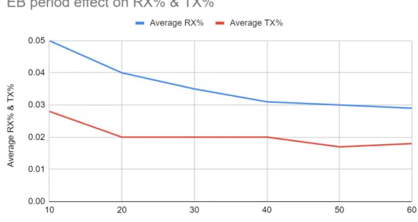
In_{figure 11 we can observe how both the average times each node is spending receiving data or} transmitting data is changed as the EB period changes. The reason we can only see the red line in figure 11 is because the blue and red lines are completely overlapping. The reason for this is because this scenario consists of only 2 nodes, so for each packet sent the receiving node has to receive it. And apparently, according to the measured values that takes the same amount of time in this case.

(26)

Figure 11 - single-hop, no mobility, eb period effect on radio TX and RX time

In_{figure 12 we have added the percentage values from the previous graphs in figure 9} , 10, and 11 and multiplied those values with the running times of each simulation for each EB period and thereby creating a graph representing the total time the average node has its radio active, either by listening (ON), receiving (RX) data, or transmitting (TX) data. We can observe that there is not much change as the EB period is increasing in this simulation scenario. On average, the graph tends to move slightly upwards as the EB period is increasing. With exception for the EB period 40 and 50 seconds. This is related to the graph in _{figure 11 since most the radio usage time seems} to come from having the radio in the ON state, that is only listening and not processing and packets by either receiving or transmitting data.

(27)

Figure 12 - single-hop, no mobility, eb period effect on total radio usage time

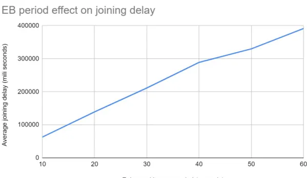
In figure 13 we can observe how the EB period affects the time it takes all of the nodes to join the TSCH network. The graph increases up until the EB period is set to 40 seconds and then it decreases. It makes sense for the joining delay to increase as the EB period is increasing since fewer EB messages are sent. We would expect the radio to stay in the ON state for longer times when the nodes are spending more time listening for EB packets but this is not the case here since we can observe in _{figure 13} that the join time is the longest for the EB period set to 40 seconds but in _{figure 10} and_{figure 12} we can not see this reflected in the radio usage time. This could be due to us entering the wrong values from the tests or for some factor for this scenario that we do not understand. In the same way we can observe in _{figure 13} that the join delay is about as low for the EB period of 60 seconds as the EB period of 30 seconds but in _{figure 10} and_{figure 12} the radio usage time and radio listening times have their greatest values.

(28)

Figure 13 - single-hop, no mobility, eb period effect on joining delay

In _{figure 14 we can see how the EB period affects the average end-to-end delay in the network.} There is a slight tendency that the average delay is decreasing in relation to a higher EB period. Since there is only 1 node connected to the RPL server there will be less messages sent in total during each run. Therefore the EB period does not seem to change much since less packets are being sent. Average end-to-end delay will therefore not change much. This effect will probably be more revealing in a simulation with more nodes connected since more traffic will flow to the server.

Figure 14 - single-hop, no mobility, eb period effect on end-to-end delay

(29)

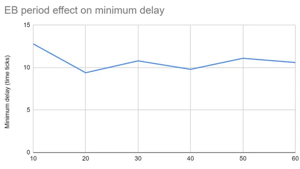
In _{figure 15 and 16 we can observe a slight increase in minimum and maximum delay} respectively. From our understanding the delay should not be increasing as the EB is increasing, since an increased EB period leads to fewer data packets being sent over the network. However, since this network consists of only 2 nodes we believe that the slight increase is not a real pattern but only the way the curve was shaped on average over the few runs we ran. This makes since because the curves are very close to being flat which suggests that the results, on average for each EB period is the same, and with only 2 nodes there will be very little data flowing through the nodes, and most likely they did not meet their maximum throughput capacity and therefore everything being sent could just be forwarded without much delay at all, except the time scheduling caused by TSCH which probably happened to be causing longer delays for the shorter EB periods in this scenario.

Figure 15 - single-hop, no mobility, eb period effect on minimum delay

(30)

Figure 16 - single-hop, no mobility, eb period effect on maximum delay 8.2 Results for the multi hop with no mobility

This scenario is slightly more complicated and realistic than the single-hop scenario presented in the previous section. This scenario consists of a 6TiSCH root node, and 9 pledge nodes as pictured in figure 2. The reason for this being more realistic is that there is often more than 1 node connected to a server. Also there will be more traffic overall introduced to the network, this will likely have a greater impact on the network in terms of latency, throughput and energy consumption. Since the scenario is considered to be more realistic, this data will be also considered to be more accurate to the reality.

In_{figure 16 we can observe the throughput decreasing just as we did in the previous scenario and} figure 9.

Evaluation of 6TiSCH network performance for SDN-enabled IoT networks

M

​

U

​

S

​

​

I

​

, D

​

​

E

​

V

​

, S

​

Thesis for the Degree of Bachelor of Science in Engineering - Computer Network

Engineering, 15 HP

Evaluation of 6TiSCH network performance

for SDN-enabled IoT networks

Adam Sandström

asm17005

​@student.mdh.se

Nico Klerks

nks17001

​@student.mdh.se

Examiner:

Mats Björkman

Supervisor:

Shunmuga Priyan Selvaraju

Supervisor:

Hossein Fotouhi

Supervisor:

Iliar Rabet

Abstract

Table of Contents

List of Figures

1.

Introduction

2.

Background

3

Related work

4.

Problem Formulation

5.

Method

6.

Ethical and Societal Considerations

7.

Experimental setup

15

​

8 Results

_{@student.mdh.se}

_{@student.mdh.se}