Fuel Efficiency in AWD-system

(1)

Fuel Efficiency in AWD-system

Robert Fredriksson

Milovan Trkulja

THESIS WORK 2008

(2)

(3)

Fuel efficiency in AWD-system

Robert Fredriksson

Milovan Trkulja

This thesis work is performed at Jönköping Institute of Technology

within the subject area mechanical engineering. The work is part

of the university’s three-year engineering degree.

The authors are responsible for the given opinions, conclusions

and results.

Supervisor: Patrik Cannmo

Credit points: 15 points (C-level)

Date: 2008-05-19

(4)

(5)

Abstract

This degree project has been made in cooperation with engineers working for GM Engineering/Saab Automobile AB in Trollhättan. The given name by Saab for the project is “Fuel efficiency improvements in All Wheel Drive(AWD)-system”. The main tasks of this thesis work were to investigate the size of the power losses in different parts on the propeller shaft, to design a computer program that calculates coordinates and angles on a propeller shaft and to investigate the possibilities to put together a simplified formula that calculates the natural frequencies on a propeller shaft.

The main parts of this report are a compilation of the theory about AWD and mostly about the parts on the propeller shaft, and also a description of the developed

computer program called Propeller Shaft Calculator. This report doesn’t concern power losses in the different joints because there were no such general equations to be found. The most common way to calculate the power losses inside a joint is to do tests were the power loss is measured at different angles, torque and speed and then use that data to put together an approximated equation.

Most of the work on this project has been on theory studies and on programming. The main result of the project is the program Propeller Shaft Calculator. Propeller Shaft Calculator is a program that is designed in Microsoft Excel. All the menus are programmed in the visual basic editor in Excel. The program is supposed to be used as a help while designing new propeller shafts.

Propeller Shaft Calculator can calculate all the coordinates, lengths, angles and directions on a propeller shaft. It also calculates natural frequencies, plunge, estimated power loss on the second shaft and angles in the joints. In the program you can choose to do calculations on four different configurations of propeller shafts but can quite easy upgrade the program with more choices.

Basically the program works like this:

First you choose the right propeller shaft in the main menu. Then you fill out the in-data sheet with coordinates, lengths, material in-data and so on. As you type in the input data the output data will appear in the out-data sheet next to the in-data. Every propeller shaft has also a calculations sheet were more detailed calculations can be found.

The program also has a built in help function and a warning function that lights a warning sign next to the values if they are outside the limits.

(6)

Key Words

GM Engineering Saab Automobile AB Car Joint Coupling XWD AWD Propeller shaft Cardan Natural frequency Program Calculation Power loss

(7)

Prefatory note

The authors would like to give a big thanks to the employer Saab Automobile for taking us in for the project. They would also thank their supervisor Mats Ullman, and all the other engineers at the AWD department for all the help that has been given through the project and has made the thesis work possible.

(8)

(9)

1 Introduction ... 1

1.1 BACKGROUND...1

1.2 PURPOSE AND AIMS...2

1.2.1 Requirement specifications ...2 1.2.2 Aims ...3 1.2.3 Assignments ...3 1.3 DELIMITATIONS...7 1.4 OUTLINE...7

2 Theoretical background... 9

2.1 SHAFTS...9 2.2 JOINTS...11

2.2.1 Cardan joint (Hooke´s joint)...11

2.2.2 CV-joints (Constant velocity joints)...12

2.2.3 Other joints ...15

2.3 LUBRICATION AND PERFORMANCE...20

2.4 NATURAL FREQUENCY ON ROTATING SHAFTS...21

2.5 POWER LOSSES DUE TO SPEED VARIATION ON A SHAFT...22

2.5.1 Calculations based on changes in kinetic energy...22

2.5.2 Calculations based on acceleration on the shaft...25

2.6 VECTOR CALCULATIONS...27

2.7 HOW 4-WHEEL DRIVE WORKS...28

2.8 SAAB XWD...29

3 Implementation... 31

4 Results... 33

5 Conclusions and discussions ... 35

6 References... 37

7 Search words... 39

(10)

(11)

1 Introduction

There is always an interest in lowering the fuel consumption within the Automotive industry because of the competition when the fuel price increases. New cars are supposed to consume less fuel all the time. The requirements on the different systems are constantly increasing. All this is carefully followed up in the development projects off new car models.

In this report a number of components in the AWD-system will be studied to se if there are any possible improvement potentials. The chosen components that will be studied are the propeller shaft, the joints and the bearings. The parts will be studied to se if they could be designed to be me more effective or if there are any better options on the market that are more energy saving.

To make the design of a new propeller shaft easier and more time saving a new computer program has been developed together with engineers at Saab Automobile. The program is made in Microsoft Excel and can calculate lengths, angles, natural frequencies, plunge and power losses on the propeller shaft.

This work has been made as a thesis work for a bachelor degree and the report together with the computer program is the result.

1.1 Background

Saab Automobile is a subsidiary company completely owned by General Motors from the year 2000.

GM has a very large enterprise in Europe and counts as the world’s largest

manufacturer within the private car segment. Saab sells about 130 000 cars in over 60 countries, and has most of its production in Trollhättan with approximately 4700 employees.

The main office is centered in Trollhättan but parts of the group operations are stationed in Gothenburg and Pixbo.

All Wheel Drive is a growing and strategically very important area within the car industry. GM is carrying out an offensive staking on this area and has established a global AWD Center in Sweden, Trollhättan. The goal is to become world leading within AWD.

Since the requirements on low fuel consumptions and lower discharges among cars are getting fierce the car manufacturers must constantly work on better solutions to make the cars more energy efficient. Fuel efficient AWD is a project in progress on Saab Automobile AB which job is to investigate all parts in the AWD cars drive train with the aim to minimize the energy losses.

This work is just a little part in a larger project and the main focus is to make a tool that simplifies concept studies and to give suggestions to improvements on the propeller shaft, joints and bearings. [9][15]

(12)

1.2 Purpose and aims

The purpose with this report is to make a tool that can make the daily work for the engineers on the AWD-department easier when redesigning propeller shafts. Instead of searching in several sources for the basic facts about different shafts, joints and calculations, all of the most important facts will be put together in one single report. A program will also be provided which can calculate the most useful data about the propeller shaft.

1.2.1 Requirement specifications

• Set up guidelines how to construct an energy effective propeller shaft. • Set up guidelines how to choose an energy effective joint.

• Set up guidelines on which bearing would be the most energy effective. • Choose the component on the propeller shaft with the highest energy losses. • Create a tool in excel that can calculate the propeller shaft angles in 3D with

the help of input of measures and coordinates.

• Create a model for the calculation of the propeller shafts natural frequency with the help of velocity, measures and material.

• Find out which suppliers that offers the most efficient components. • Write the report of the work in English.

(13)

1.2.2 Aims

• Obtain deeper knowledge about the chosen parts on the propeller shaft to find the greatest causes to power losses and to give proposals how these can be reduced.

• Write a report with facts about the propeller shaft and its components that can be used as a support while designing an efficient driveline.

• Create a program that calculates the different angles and directions between the parts on the propeller shaft after inserted specific data.

• Create a model for calculating the natural frequency of the propeller shaft. • Get to know engineers within the Automotive industry.

• Learn how a modern AWD-system works.

• Increase the knowledge about the car manufacturing industry.

1.2.3 Assignments

These are the assignments that will be done in the respective areas.

Planning

• Project description • Background • Goal/Purpose • Requirements Specification • Procedure

(14)

Theory studies of AWD-components

• Bearings • Joints

• Propeller shaft

• Suspension mounting for support bearings

Investigate energy losses and causes to these

• Bearings – (e.g. dimension, friction, vibration, lubrication) • Joints – (e.g. angle, vibration, mass, friction, dimensions) • Propeller shaft – (e.g. vibration, mass, dimensions, material)

• Suspension mounting for support bearings – (e.g. material, dimensions, vibration, hardness)

• Develop a tool to calculate angles on propeller shafts

• Work with a tool or a formula to estimate the natural frequency on the propeller shaft

• Identify the most critical component.

Investigate alternative solutions/improvements for each component

• Study competing companies – Racing/Private cars • Study other similar applications.

• Contact subcontractors for information – Future/Other solutions/Aware of problems

(15)

Further development of chosen critical component with the greatest

improvement potential

• Perform calculations • (Simulations) • (Prepare tests)

Result control

• Investigate the reasonableness of a solution.

-Cost, delivery time, subcontractors, advantages/disadvantages. • Reliability control.

Report writing

• Report parts • Disposition • Dependency • Pictures – Copyright • Diagrams • References • Draft • Copy-typing • Check-up • Secrecy

(16)

Presentation

• Disposal • PowerPoint • Copyright

Disputation

• Opposition on group.

Printing

• Print at least 2 hardback copies + 1 loose-leaf

Follow-up

• What went good/bad

• Did the goals and requirements get fulfilled • Can the result be used or develop further

(17)

1.3 Delimitations

The degree project will not consider the area about natural oscillation on a shaft with a suspension mounting because those calculations are far more complex than those for a stiff mounted shaft. These calculations would also be very hard to make into a

universal equation that could be used in a computer program. This report won’t either go into the area of power losses in joints or suspension mountings because no such equations could be found during the project. There wasn’t enough time in this project to find those equations through different laboratory tests so the time had to be

prioritized for the development of the computer program instead. The same goes for calculations concerning bearings were we assumed that the power losses would be very small.

There aren’t any price comparisons made between the different joints because the joint manufacturers that were contacted didn’t want to leave out any prices.

1.4 Outline

This report has four main parts. First is the introduction part. Then comes the biggest part of this report which is the theoretical background. Here are all the facts that have been put together. The third big part is the result together with the conclusions. Here is all the information about the developed computer program. The last main part is the attachments. Most of the important calculations for the program and the instruction manual are some of the documents that can be found here.

The theoretical background together with the development of the “Propeller Shaft Calculator” has been most essential for this project and its result. The result will not be very deeply presented in the paper because it’s a computer based program made in Microsoft Excel. The program will be handed in separately on a CD to Saab and if permission is given by Saab then the school will get a copy as well.

(18)

(19)

2 Theoretical background

The theoretical background contains all the facts for the respective area that has been found in books, on the internet and in documents at Saab. Here is theory for shafts and joints, calculations on natural frequency on tubes, power losses due to speed variation on a shaft, lubrication and performance, 4WD, Saab XWD.

2.1 Shafts

The most commonly used shaft to transfer torque between the gearbox and the rear axle on cars is the propeller shaft, also called cardan shaft. The name cardan comes from the famous Italian professor and mathematician Geronimo Cardano (1501-1576).

The first shafts that were used were solid shafts. Those aren’t very good because they are heavy, they don’t allow any axial movements between the gearbox and the rear axle and they transmit a lot of vibrations. Due to these problems the new shafts had a different design. They were hollow to save weight, and also had the ability to plunge (a sliding ability so that the length can vary). Even later the shaft was divided into two and three shorter shafts with joints mounted to the chassis between them. The reason for this was to prevent the shaft from working in the range of natural frequency which would make it vibrate.

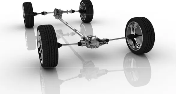
The main task for an axle is to transfer torque and rotation. Two of the axles on the car that transfer most torque are the propeller shaft that transfer torque between the gearbox and the differential and the drive shaft that transfer torque between the differential and the wheel hubs.

A shaft in the driveline of a car should be designed to be able to transfer the given amount of torque during the whole life of the car without any maintenance. Other demands on the shaft are that it should neither produce nor transfer vibrations. It should also have low losses of energy and be as light as possible.

Shafts that have direct contact with the wheels are called unsprung mass. These shafts have even higher demands on their weight and vibration properties.

On some shafts there are mounted a vibration absorber to reduce the vibrations. A disadvantage with these is that they increase the total weight of the shaft.

The shafts in the driveline of the car are mostly manufactured from steel, but also aluminum and composites are used.

When calculating the dimensions of a shaft it’s important to take fatigue failure and stability into consideration. This means that calculations should be made with varying load and also different kinds of loads like bending, torsion and tension.

(20)

One method to use when you are dimensioning a shaft is to first do approximate calculations for both the shaft and the bearings. When that’s complete, continue with more accurate calculations. First when the shaft is setting the design load and then when the bearing is setting the design load. Calculations should be made for both static and dynamic loads.

When calculations are done on a shaft with statically stated bearings were the load is setting the dimensions you should do a force- and a torque-graph.

When calculating and the deformations are setting the dimensions, it should also include deformation relations in the calculations.

While calculating on a shaft with statically unstated bearings it should also include the geometrical relations. [2][3][5][11][12][13][14]

(21)

2.2 Joints

A joint is supposed to transfer torque and rotation between two shafts. There are many different kinds of joints for different applications. When choosing a joint for a specific use then following issues has to be considered: [3][6][11][13]

• Use

• Kind of joint • Motion

• Forces and torque • Driving conditions • Running speed • Design

• Dimensions and weight • Environment

• Assembly and dismounting • Replacement

• Length of life • Price

2.2.1 Cardan joint (Hooke´s joint)

The cardan joint consist of a cross, where each shaft end is connected through bearings with the two opposite arms of the cross. There are different kinds of cardan joints on the market. In some designs the cross is replaced by a ball. One disadvantage with the cardan joint is that the rotational speed on the output axle is pulsating when you bend the joint. The size of the pulsations in rotational speed is depending on the bending angle and this causes vibrations. The nominal angle should be between 0,6 and 6 degrees according to GM best practice. The maximum angle should never exceed 20 degrees. During one revolution the second axle is going through two phases of accelerating and retardation. An equation for the angular speed on the second axle is shown below. α ϕ α 2 1 2 1 2 sin cos 1 cos ⋅ − ⋅ Ω = Ω Equation 2.1 Where:

Ω1=Angular speed shaft 1

Ω2=Angular speed shaft 2

α=Deflection angle between shafts φ1=Rotational angel shaft 1

(22)

The angular speed on the second shaft is highest and lowest for these values of φ1: α ϕ cos 1 180 0 max 1 2 1  =      Ω Ω ⇒ ° ° = Equation 2.2 α ϕ 90 90 cos min 1 2 1  =      Ω Ω ⇒ ° − ° = Equation 2.3

To counteract the pulsations on the second shaft mounted to the rear axle it is possible to assemble two cardan joints with a middle shaft. The result is three shafts and two cardan joints. The first and the third shaft then get constant speed. To get this working it is important that the U-shaped claws on the middle shaft-ends are mounted right depending on the angles in the joints, otherwise the pulsations will be even greater. The main reason that the cardan joint is used to a great extent in spite of the pulsations is because of its relatively high efficiency, and because it’s often used with small angels which doesn’t give very large pulsations. However it’s important that the joint isn’t working without any angel at all because the lubrication would then fail.

[3][4][6][8][11][13][14][17]

2.2.2 CV-joints (Constant velocity joints)

CV-joints are able to transfer torque with constant angular speed even in quite large angles. These joints are more effective than cardan joints when it’s necessary with large angles. [11]

2.2.2.1 Ball joints (Rzeppa-joints)

The ball joint is the most commonly used joint on FWD cars. It consists of an inner and an outer half with tracks for balls that transfer the torque between the two halves. Except for FWD-cars this joint is also used on RWD and AWD cars. The appropriate angles for different kinds of ball joints varies. The nominal angle should normally lie between 1 and 6 degrees. The maximum angle varies for different joints and it can be up to about 50 degrees.

(23)

Some different kinds of ball joints are: • AC (Angular Contact) Fixed Joint

This joint is useful in passenger cars and lighter vehicles. This joint can work up to 45 degrees. This joint is practical when high motions are needed for example on the front wheels.

• UF (Undercut Free) Fixed Joint

The UF joint can be used for similar applications as the AC joints. The advantage is that it can work with larger angles.

Figure 2.2 - Ball joint

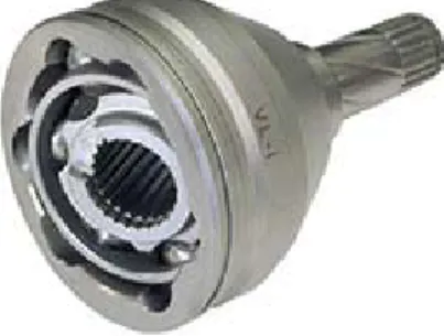
• VL (Verschiebegelenk Löbro) Disc Joint

The VL joint can work in great angles and does also admit some plunging motion. This is good when you have motions in the driveline or want to lower the assembly tolerances. This joint has very good performance on high rotational speeds. VL Disc joint is often mounted to the gearbox with a flange coupling.

Figure 2.3 - VL disc ball joint

• VL (Verschiebegelenk Löbro) Monoblock Joint

The VL-Monoblock joint is mounted to the gearbox or to the wheel hub with a shaft. It has a very compact design which saves space and weight.

(24)

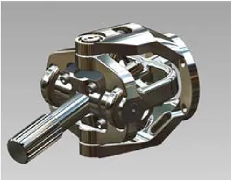
• DO (Double Offset) Joint

The DO joint is similar to the VL joint and allows high plunging motions up to 50mm and working angles up to 30 degrees. This joint has also similar

properties as the tripod joints. One advantage to the tripods is the low rotational lash which improves the NVH (noise, vibration, harshness) properties. [7][11]

Figure 2.4 - DO ball joint

2.2.2.2 Tripod joint

One alternative to the ball joint is the tripod joint. It consists of an inner part with three short shafts with bearings and an outer part with tracks for the bearings. This joint demands very low forces for plunging. This prevents vibrations to be transmitted trough the joint and does also give lower power losses when working in large angels than the ball joint. One disadvantage with the tripod joint is that it has a play in rotational direction. This can cause NVH. The tripod joints are used for relatively small angles and for applications that requires great plunging motions. One example is in AWD vehicles where the tripod joint is used to prevent vibrations and movements from the engine and the drive train to be transmitted into the car.

Some different kinds of tripod joints are: • GI (Glaenzer Interieur)

The GI joint is suitable as inner joint on the drive shafts on most vehicles. It has a working range up to 20 degrees and allows plunging up to 50mm. The low plunging forces in the GI joint gives good NVH properties.

(25)

• AAR (Angular Adjusted Roller)

The AAR joint has the same plunging length and can manage larger angles than the GI joint and has even lower plunging forces. This improves the NVH properties even more. [7][8][11]

2.2.3 Other joints

This paragraph is about new CV-joints that were found on the internet. These joints seem to be quite new. There have not been any facts found that these joints are being used in mass produced cars but if they are as good as the manufacturers say they should be suitable as a substitute to ordinary universal and CV-joints. All facts about these joints are collected from the respective manufacturer’s website.

2.2.3.1 Thompson Constant Velocity Coupling

The Thompson Coupling is essentially two Cardan joints assembled coaxially where the cruciform-equivalent members of each are connected to one another by trunnions and bearings which are constrained to continuously lie on the homokinetic plane of the joint.

At tests carried out by the manufacturer, The Thompson Coupling outlasted its rivals and it needed 9.3% less energy to do the same job, promising significant energy and fuel savings. [18]

Advantages according to the manufacturer

• The Thompson Coupling is the world's first and only true CV-joint: • Has all loads carried by roller bearings

• Has no sliding or skidding surfaces whatsoever

• Can tolerate axial and radial loads without degradation • Constructed to any torque level

• Does not require special lubrication • Does not require a dust boot

• No wearing components except replaceable bearings and trunnions • Is suitable for automotive tail or propeller shaft applications • Is less bulky than a double coupling or double Cardan joint. [18]

Disadvantages according to the authors

• The size? The minimum size is limited by the bearings.

• The price? No price comparisons between ordinary joints and the Thompson Coupling are made but the coupling is quite advanced and consists of many parts so the price should be quite high.

• The Thompson coupling does not allow any plunging movements. • The accessibility. Because it’s a quite new invention there is no mass

(26)

Manufacturing

In mass production each and every component of the Thompson Coupling can be produced by forging and/or casting with the only further requirement being to drill and machine the bearing journals, holes and circlip grooves.

No dedicated machinery is required as is the case with Rzeppa type joints. The assembly is simple but there are many parts. The bearings for most of the applications are standard bearings.

The Thompson Coupling has essentially the same construction as a normal Cardan joint but does not suffer the dynamic loads due to fluctuating angular velocity of intermediate shafts as is the case where Cardan joints are used.

The Thompson Coupling is very compact and may be over-engineered to increase reliability without adding substantially to bulk and weight. [18]

(27)

2.2.3.2 The Cornay Universal Joint

The Cornay Universal joint has a compact and balanced design, higher torsional rigidity, a great resistance to deflection and good lubrication. [19]

Advantages according to the manufacturer compared to a traditional universal joint

• True constant velocity at all angels • High torque loads

• High RPM`s

• Angles up to 90 degrees

• 65% less vibration than a universal joint • Little required space

• Low maintenance • Long service life • Price

• No boot required [19]

Disadvantages according to authors

• It rotates in a strange way which seems to produce vibrations.

• The price? No price comparisons between ordinary joints and the Cornay universal joint are made.

• Maximum speed is 5000 rpm for the Cornay 30 degree CV joint according to the website. Max rpm on the propeller shaft is more than 5000 rpm.

The Cornay Universal Joint design is said to give major performance improvements in every area where traditional universal joints suffer weaknesses.

• It‘s designed specially for high-speed, high-torque, high-angle applications that no existing joint could handle.

• Recent developments, including a newly patented centering device, allow the joint to work at a constant velocity.

• It can operate up to 98% efficiency at angles up to 90 degrees. A double Cornay joint can eliminate a gearbox in many applications.

• It handles high torque loads at high rpm, even at large angles.

• Vibrations are decreased up to 65%, thanks to concentrated mass and the balance of its concentric design.

• It increases longevity and reliability. Its unique channeled ring-type bearing housing maintains a constant supply of lubricant to all bearing surfaces and is completely purge able. [19]

(28)

Figure 2.7 - Cornay universal joint

(29)

2.2.3.3 Hardydisk

The hardydisk consist of rubber and flanges and it is used when small angles are needed. It has very good damping properties and the hardness of the rubber can be altered. The construction of the hardydisk is very simple and effective but it has some flaws such as it can only be used with small angles, nominal angle is 1 degree and maximum angle is 3 degrees. After a long time of usage the rubber tends to dry and it has to be replaced to keep the properties. [9]

Figure 2.9 - Hardydisk

(30)

2.3 Lubrication and performance

The efficiency and the performance of a joint are determined by the following parameters:

• Weight

• Variations in rotational speed • Friction

• Vibrations • Heat resistance • Tolerances

To lower the weight it’s necessary to use as small and compact joints as possible. This put high demands on the materials that have to have high strength and low density. To avoid variations in speed, a constant velocity joint can be used or design the car so that there are very small angles between the shafts. The joint should also have very good tolerances so there will be no lash which could give vibrations. This puts high demands on the manufacturing process and will also increase the price. It is also important to avoid friction and grinding in the joints to avoid power losses and wear. To keep the friction low and to avoid unwanted wear it is important that the joint is designed so that all parts are properly lubricated during all working conditions. Another disadvantage with friction except power losses and wear is the generation of heat. The hotter the joint will get the higher the demands on the grease or oil will get. The properties of the lubricant are depending on the ingredients which are oil, thickener and additives. [3][6][11][13]

(31)

2.4 Natural frequency on rotating shafts

If the shaft gets in the range of its natural frequency then it will start to vibrate and possible even cause noises. The shafts natural frequency depends on material, thickness and the length. The longer the shaft is the lower natural frequency will be. Almost every object with a natural frequency also has others, more higher

frequencies.

Following calculations on the natural frequency applies on a rotating, free laid up, round, thin-walled shaft.

Input data:

La=Length (m)

D=Outer diameter shaft (m) d=Inner diameter shaft (m) Ea=Young’s modulus (Pa)

ρa=Density (kg/m3)

Calculations:

The shafts mass, ma (kg): [12]

(

)

4 2 2 _d D L m_a = _a⋅ρ_a⋅π⋅ − Equation 2.4

The shafts moment of inertia, Ia (m4): [4][12]

) ( 64 4 4 _d D I_a = π ⋅ − Equation 2.5

The shafts natural frequencies, ωen (rad/s): [4][17]

3 2 2 a a a a en L m I E n ⋅ ⋅ ⋅ = π ω Equation 2.6 n = 1, 2, 3, 4, …

Equation 2.4 and Equation 2.5 inserted into Equation 2.6 yields:

4 2 2 2 2 16 ) ( a a a en L d D E n ⋅ ⋅ + ⋅ ⋅ = ρ π ω Equation 2.7

(32)

2.5 Power losses due to speed variation on a shaft

Following calculation will only calculate the energy that is used when a shaft between two cardan joints accelerates and retards due to the pulsations in the angular velocity that occurs in-between the input and output shaft due to deflecting angle.

2.5.1 Calculations based on changes in kinetic energy Input data:

nin=rpm

α=Deflecting angle Ra=Outer radius shaft

ra=Inside radius shaft

Rk=Radius joint la=Length shaft lk=Length joint ρa=Density shaft ρk=Density joint Calculations:

Angular velocity, ωin (rad/s), on input shaft: [12]

in in in n n ₌ _⋅ ⋅ = 6 60 360 ω Equation 2.8

Highest/ lowest angular velocity on output shaft at constant velocity on input shaft: [3][4][17] α ω ω cos max ín ut− = Equation 2.9 α ω ω_ut₋_min = _incos Equation 2.10

Mass moment of inertia shaft, Ja (Kgm2): [12]

2 2 2 a a a a r R M J = + Equation 2.11

(33)

Approximated mass moment of inertia joint, Jk (Kgm2): [12] 2 2 k k k R M J = Equation 2.12 Mass shaft, Ma (kg): [12]

(

2 2

)

a a a a a l R r M =ρ ⋅ ⋅π − Equation 2.13

Approximated mass joint, Mk (kg): [12]

2 k k k k l R M =ρ ⋅ ⋅π ⋅ Equation 2.14

Difference in angular velocity on middle shaft, ∆ωut (rad/s):

min max − − − = ∆ωut ωut ωut Equation 2.15

Equation 2.9 and Equation 2.10 into Equation 2.16 yields:       ₋ = ∆ α α ω ω cos cos 1 in ut Equation 2.16

Equation 2.8 into Equation 2.16 yields:

      ₋ ⋅ = ∆ α α ω cos cos 1 6 _in ut n Equation 2.17

Kinetic energy, Wk-a (J), to accelerate the shaft with ∆ωut: [12]

2 2 ut a a k J W ₋ = ⋅∆ω Equation 2.18

Kinetic energy, Wk-k (J), to accelerate the joint with ∆ωut: [12]

2 2 ut k k k J W− = ⋅∆ω

(34)

Kinetic energy, Wk (J), to accelerate the shaft and joint with ∆ωut: k k a k k W W W = ₋ + ₋ Equation 2.20

Equation 2.18 and Equation 2.19 into Equation 2.20 yields:

(

a k

)

ut k J J W = ∆ + 2 2 ω Equation 2.21

Equation 2.11, Equation 2.12 and Equation 2.17 into Equation 2.21 yields:

(

)

(

2 2 2

)

2 cos cos 1 3 in a a a k k k n M R r M R W _ ⋅ + + ⋅            ₋ ⋅ = α α Equation 2.22

(

)

(

4 4 4

)

2 cos cos 1 3 _in _a _a _a _a _k _k _k k n l R r l R W _ ⋅ ⋅ ⋅ − + ⋅ ⋅ ⋅            ₋ ⋅ = α ρ π ρ π α Equation 2.23

The frequency, f, for the pulsations on the middle shaft (the shaft will accelerate and retard two times per evolution): [12]

15 60 4 nin nin

f = ⋅ =

Equation 2.24

Power loss, Ptot, due to the pulsations: [12]

k tot f W

P = ⋅

Equation 2.25

(

)

(

4 4 4

)

2 3 cos cos 1 5 3 k k k a a a a in tot l R r l R n P  ⋅ ⋅ ⋅ − + ⋅ ⋅ ⋅      ₋ ⋅ ⋅ = α ρ π ρ π α Equation 2.26

(35)

2.5.2 Calculations based on acceleration on the shaft Input data:

nin=rpm

α=Deflecting angle Ra=Outer radius shaft

ra=Inside radius shaft

Rk=Radius joint la=Length shaft lk=Length joint ρa=Density shaft ρk=Density joint Calculations:

Angular speed of propeller shaft, ωin (rad/s): [12]

30 60 2π π ω = in⋅ = in⋅ in n n Equation 2.27 Mass of shaft, Ma (kg): [12]

(

2 2

)

a a a a a l R r M =ρ ⋅ ⋅π − Equation 2.28

Approximated mass of joint, Mk (kg): [12]

2 k k k k l R M =ρ ⋅ ⋅π ⋅ Equation 2.29

Mass moment of inertia shaft, Ja (Kgm2): [12]

2 2 2 a a a a r R M J = + Equation 2.30

Approximated mass moment of inertia joint, Jk (Kgm2): [12]

2 2 k k k R M J =

(36)

(

)

2 4 4 a a a a a r R l J = ρ ⋅ ⋅π − Equation 2.32

2 4 k k k k R l J = ρ ⋅ ⋅π⋅ Equation 2.33

Equation 2.32 + Equation 2.33 yields total mass moment of inertia, J(Kgm2):

(

)

2 2 4 4 4 k k k a a a a k a R l r R l J J J = + = ρ ⋅ ⋅π − + ρ ⋅ ⋅π⋅ Equation 2.34

Resulting inertia torque in propeller shaft, Minertia (Nm): [17]

2 2 2 2 2 ) sin sin 1 ( 2 sin sin cos 2 ϕ β ϕ β β ω − ⋅ ⋅ = in inertia J M Equation 2.35

Equation 2.27 and Equation 2.34 into Equation 2.35 yields:

(

)

2 ₂ 2 ₂ ₂ 4 4 4 ) sin sin 1 ( 2 sin sin cos 30 ) ( ϕ β ϕ β β π π ρ π ρ − ⋅       ⋅ ⋅ ⋅ ⋅ ⋅ + − ⋅ ⋅ = in k k k a a a a inertia n R l r R l M Equation 2.36

(37)

2.6 Vector calculations

Figure 2.9 - A vector in A3

A vector v in A3 (three dimensions) consists of an X, a Y and a Z component. A vector v between the coordinates P1 and P2 in A3_{is calculated with the following}

equation: [1]           =           − − − = Z Y X Z Z Y Y X X v v v P P P P P P v r r r r 1 2 1 2 1 2 Equation 2.37 The dot product between the vectors u and v is: [1]

Z Z Y Y X X v u v u v u v ur• r= →⋅→ + →⋅→ + →⋅→ Equation 2.38

| v | is the length of vector v and is calculated with the following equation: [1]

2 2 2 | |vr = vrX +vrY +vrZ Equation 2.39

The angle α between vectors u and v are calculated with the following formula: [1]         ⋅ • = − _→ _→ | | | | cos 1 v u v u rr α Equation 2.40

Vector vu is the projection of vector v on vector u and is calculated with the following formula: [1]

→ →

(38)

2.7 How 4-Wheel Drive works

A 4WD car is always superior a 2WD car when you are comparing the grip while accelerating or driving through a curve. But 4WD doesn’t always mean that all wheels drift at all times. The worst case scenario is that the car could drift only on 1 wheel. If one wheel is spinning on ice and the rest are standing still on rough ground. Some different kinds of 4WD and some terms concerning 4WD will be explained below. Disconnect able 4WD:

This is the original and simplest form of 4WD. Normally on asphalt the car is 2WD, generally RWD (Rear Wheel Drive). But with a so called dispursion box (an extra gearbox) the FWD (Front Wheel Drive) can be connected and the car gets 4WD. Constant 4WD:

It’s getting more common with constant (permanent) 4WD. The advantage is that the cars chassis can be optimized for just only 4WD and the driver doesn’t have to think about when ether or not he has connected the 4WD. Cars with constant 4WD

sometimes call their system for AWD (All Wheel Drive). Differentials:

A car driven on the road must have differentials in the axles. When the car turns in a curve then the outer wheels travels a longer distance and spins faster than the inner wheels. The differentials in the axels consists of a system of cog pinions that allows the right and the left driving shafts and with that the wheel spinning at different speed. If the “open” differentials did not exist then the axles would “tie it self” and the steering would be very heavy. The mechanical tensions in the driving shafts could make them break.

Middle-differential:

A car with 4WD must also have a middle-differential (central differential) – a differential between the front and the rear propeller shaft. Because in a curve it’s not just the outer and the inner wheels that spins at different speed, but also the front and the rear wheels. Even when driving straight forward the wheel can spin at different speed depending on how much the wheels are worn out. The middle-differential allows the front and the rear axle to revolve at different speed which prevents the transmission to “tie it self”.

Haldex coupling:

The Haldex coupling is the latest within 4WD-system. It's a Swedish invention from the beginning and it consists of a multiple-plate lamella coupling that lies in an oil bath along with an electronically maneuvered pump-piston system. The pressure from the pumps affects various different sensor-cylinders where the pistons press the lamell-package together so that the force can disperse between one axle to another. The system reacts very fast and has the advantage to quickly disperse the driving-force to the axle (wheel) with grip. [16]

(39)

2.8 Saab XWD

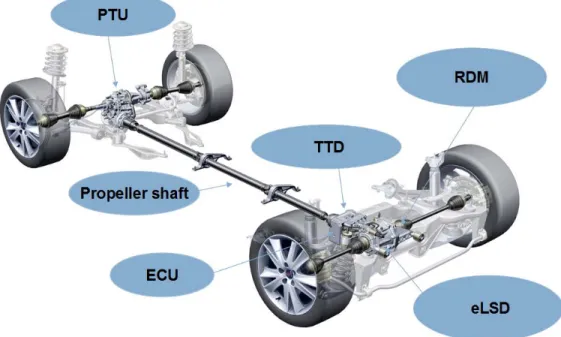
The XWD (Cross Wheel Drive) system that is used in the new Saabs is a high torque, active on demand AWD (All Wheel Drive) system. The XWD system helps the driver to stabilize the car while driving fast through curves or while changing lanes very quickly. The system gives stability at high speed and throttle off. The pre-emptive function adds the possibility to fully engage the XWD system before takeoff to maximize the acceleration. That gives massive traction and no front wheel spin, and also a mechanical stiffness feeling like a permanent XWD system. The XWD system can be tuned for different handling characteristics, under steer, neutral or over steer. It uses among others the engine torque, wheel speed signals and the yaw rate sensors to know the vehicles movement. The XWD system also uses the pre-emptive function to increase the possibilities for handling.

Figure 2.10 - Complete XWD system

First, the gearbox transfer torque to the front axle. The PTU (Power Take-off Unit) then transfer torque from the front axle to the propeller shaft. The propeller shaft is transferring torque from the PTU to the TTD (Torque Transfer Device). The TTD contains a clutch which distributes torque between the front and rear axles. The TTD is connected to the RDM (Rear Drive Module) which contains the rear differential. On some models there are an eLSD(electronically controlled Limited Slip

Differential) mounted to the RDM. The eLSD contains a clutch that distributes torque between the rear wheels. The locking level of both the TTD and the eLSD are fully controllable between 0 and 100%. It’s the ECU (Electronic Control Unit) that is assembled to the TTD, which controls the pressure on the clutches in the TTD and the eLSD. The ECU is collecting data such as wheel speed, steering wheel angle, yaw rate, acceleration, ABS signals, ESP signals, engine speed and engine torque from the

(40)

The eLSD increases the traction and helps the driver at cornering and throttle off situations like avoidance maneuvers.

This XWD system is compatible with 5 different engine families and 3 different transmission families that are used within GM. The software is tunable for the different brand characters and the system is fully integrated in the ESC (Electronic Stability Control). The system can also be tuned for yaw damping if necessary.

Figure 2.11 – The parts of the AWD system

The system has an electro-hydraulic system with an electrical hydraulic pump and one or two electronically controlled hydraulic valves that control hydraulic pressure to the TTD and the eLSD couplings. The oil is first pushed through a paper based oil filter – and then to an accumulator. The accumulator stores the pressure, and thereby speeds up the system when pressure is quickly needed.

There are PWM (Pulse Width Modulation) controlled valves for the TTD (Torque Transfer Device) and the eLSD, both feed by the same pump/accumulator. The valve controls the oil pressure to a piston that presses on a clutch pack, and when the clutch pack is pressed, it transfers torque. [9][10]

(41)

3 Implementation

This thesis work is executed during the spring semester of 2008. Most of the work has been done in the office at Saab. The first weeks were spent on planning and

discussions what to do, how to do it and when. When all the documents concerning goals, background, assignments and background where done a detailed time table in form of a GANTT-schedule was made.

After this was done the theoretical studies begun. Literature about, joints, propeller shafts and bearings from different books where put together. The literature was also complemented with information from different websites. Questions about facts were asked to the employees at GM, competitors and subcontractors. Previous calculations made by engineers at GM were studied to make it easier to get started.

Next step was to start with the calculations concerning power losses and try to find the greatest source to power losses on the propeller shaft. Calculations concerning natural oscillation on shafts were made parallel as the calculations of power losses.

At first all calculations were made by hand to find the most efficient way to calculate the angles on the propeller shaft with as few input data as possible.

When most of the facts and the calculations were found the development of a excel program for calculations on propeller shafts started. This was the main part of the thesis work and took several months. The first version of the program did only include one model of a propeller shaft and did only calculate the angles in the joints and the lengths between the different coordinates. As the first version seemed to work well the program was developed further and included more versions of propeller shafts and more output data then the first version. The program was also made more user

friendly with buttons, a main menu and a help menu. Between every large change with the program engineers on the AWD-department (All-Wheel-Drive) were asked for ideas and critics. Tests that the calculations in the program were correct were also carried out between the main changes.

Along with the development of the excel program research were made to find more information about joints and propeller shafts. This research included literature studies of more specialized books and comparisons to other calculations made.

The last work on this thesis was to finish the report together with the presentation material. This was mostly carried out at Jönköping University. The final account was held first at Saab in Trollhättan and later at Jönköping University. After the final account at Jönköping University only correcting and adjustments of the report and printing of the finished report remains.

(42)

(43)

4 Results

After have done the studies and calculations along with the developing of the calculation program for the propeller shaft, the final conclusion regarding fuel efficiency has been established from the authors and Saab’s point of view. The conclusion is that the power losses in the propeller shaft are insignificant when acceptable angles are used to get the right design.

However if the acceptable maximum angles are slightly increased the power losses will also increase exponential, which concludes that the changes can easily be seen in the program.

When talking about power losses in the different joints it’s not simple to get an answer. To get to this information, experimental test methods are needed to establish equations for each joint. And so far no information has been found regarding

equations on power losses in joints.

The excel program that has been named “Propeller shaft Calculator” is the final product in this degree project. It took approximately four months to complete the final version. All the versions were tested by the engineers that we had contact with, and after each testing a briefing meeting was held so that they could give feedback and that the program could be updated following their demands.

The program is based on advanced excel programming for the calculation part while including visual basic programming for the appearance part of the program. It consists of many sheets which basically are the different layouts of propeller shafts that can be chosen in the main menu of the program. Every layout consists of two sheets, the first one is called “in data/out data” where you put in your obtained information and then look at the outcome.

The second sheet is called “calculations”, here is more detailed information that are not shown in the “in data/out data” sheet and here is where all the calculations are done before the result is exported to output data.

There are two kinds of layout sheets for each of the propeller shaft and the second one ends with “CAD”. The main difference between these two is that if you for example have the lengths on the shafts as input data you will choose the first layout, however if you don’t have the lengths and must use a CAD program to get the coordinates of the shaft you have to use the second layout ending with “CAD”.

To see more detailed information about how the program works then there is an instruction manual attached to the paper in the attachment section.

(44)

(45)

5 Conclusions and discussions

The goal with this degree project was to get both general and deep knowledge about the AWD-system. The general part was mostly about how the AWD-system works in practice and which components that are involved. The deeper knowledge was to learn more about a specific part namely the propeller shaft and its components, this was decided from the beginning by Saab. The main problem was to find out if there were any power losses due to the design of the propeller shaft or its components and how these can be reduced.

With the final product “Propeller Shaft Calculator” completed the authors feel that the goal was fulfilled in many ways. The part from learning about the AWD-system and the propeller shaft, the authors has also made great connection with many engineers in the AWD-department.

After having a guided tour through the Saab factory where the cars are assembled the authors got a better insight in how the production works and how they work together with the technical department that includes the AWD department.

Also having test-driven the new Turbo X helped us understand how the AWD-system responds in practice.

Regarding the power losses in different joints that couldn’t be solved at the moment, the authors have put forward some suggestions on how to get to that information. By setting up the different joints in some kind of testing device that could measure the power losses and from there equations can be made for each joint.

General calculations on power losses on bearings were made but they were so insignificant that the authors choose not to include them in the thesis work. Both the authors and Saab agree that the “Propeller Shaft Calculator” works and compared to data from subcontractors the results is almost exact. However Saab feels that the program could be filled out with more propeller shaft layouts later on but for now it’s enough to work with.

(46)

(47)

6 References

[1] Adams, Robert. A (2003) Calculus a complete course, fifth edition ISBN 0-201-79131-5

[2] Dahlberg, Tore (2001) Teknisk Hållfasthetslära, tredje upplagan, Studentlitteratur, 2001, ISBN 91-44-01920-3

[3] Eriksson, E; Kassfeldt, E; m.fl. (1993) Maskinelement. Siriuslaboratoriet, Luleå tekniska universitet.

[4] F.Schmelz, Count H.-Chr.Seherr, E.Aucktor (1991) Universal Joints and Drive shafts (Analysis, Design, Applications),Springer-Verlag, 1992,

ISBN 3-540-53314-1, ISBN 0-387-53314-1 [5] Gerbert, Göran (1993) Maskinelement del A

Maskin- och fordonskonstruktion, Chalmers tekniska högskola.

[6] Gerbert, Göran (1993) Maskinelement del B Maskin- och fordonskonstruktion, Chalmers tekniska högskola.

[7] GKN-Driveline (2008), http://www.gkndriveline.com (Acc.29/01/2008 ) [8] GM Best practice: Id 111066

Id 109024

Id 102147

Id 102158

[9] GM Europe AWD Center Trollhättan

[10] Haldex (2008), http://www.haldex-xwd.com (Acc.23/04/2008 )

[11] Landsberg; Lech (1998) Constant velocity driveshafts for passenger cars.

Verlag Moderne Industrie, D-86895

[12] Lindström, Bo; Mårtensson, Nils; m. Fl. (1992) Karlebo handbok, utgåva 14. Liber, 1992, ISBN 91-21-13273-9

(48)

[14] Robert Bosch GmbH (2004), Bosch Automotive Handbook, 6th edition ISBN 0-7680-1513-8

[15] Saab Automobile AB (2008), http://www.saabsverige.com/main/SE/sv/ (Acc.28/01/2008 )

[16] Sweden offroad (2008),

http://www.swedenoffroad.com/sv/skola/4hjulsdrift.html (Acc.14/05/2008 )

[17] The society of Automotive Engineers, Inc. Universal Joint and Driveshaft Design Manual (1979), Advances in Engineering series No.7

[18] Thompson Couplings Limited (2008) http://www.cvcoupling.com (Acc.04/03/2008 )

[19] Universal drive technologies (2008), http://www.universaldrivetech.com (Acc.18/03/2008 )

(49)

7 Search words

A Abstract ...I Aims ...3 Assignments...3 Attachments ...41 B Background ...1 Ball joints ...12 C Cardan joint...11 Conclusions and discussions ...35 CV-joints...12 D Delimitations...7 G GANTT Schedule ...67 Gates...73 H Hardydisk ...19 How 4-Wheel Drive works...28 I Implementation ...31 important formulas...66 Instruction-Manual...55, 57 Introduction...1 J Joints ...11 L

Lubrication and performance...20 N

Natural frequency on rotating shafts...21 O

Outline...7 P

Power losses due to speed variation on a shaft ...22 R References ...37 Requirement specifications...2 Results ...33 Rzeppa-joints...12 S Saab XWD...29 Shafts ...9 T Table of Contents ...V The Cornay Universal Joint ...17 Theoretical background ...9 Thompson Constant Velocity Coupling ...15 Tripod joint...14 V,W

(50)

(51)

8 Attachments

Attachment 1 - Vector calculations for the program Attachment 2 - Instruction manual for the program Attachment 3 - GANTT Schedule

(52)

(53)

ATTACHMENT 1

(54)

2-PIECE SHAFT WITH PLUNGE IN FRONT

Figure 8.1 - Coordinates on a propeller shaft

Input data: P0, P1, P4, P5, P6, |2.3|

→

, ||3→.4 , ||4→.5

Vector 0.1 (CVJ1) and its length is calculated between centre of mating surface on CVJ1 and front endpoint CVJ1.

| 1 . 0 | 1 . 0 1 0 → → ⇒ − = P P

Vector 5.6 (CVJ2) and its length is calculated between centre of mating surface on CVJ2 and joint centre CVJ2.

| 6 . 5 | 6 . 5→ = P₆−P₅ ⇒ →

Vector 4.5 (shaft 2 rear) and its length is calculated between joint centre CVJ2 and centre of support bearing.

| 5 . 4 | 5 . 4 5 4 → → ⇒ − =P P

Vector length 3.4 (shaft 2 front) is calculated. | 5 . 4 | | 5 . 3 | | 4 . 3 | → = → − →

Vector 3.4 (shaft 2 front) is calculated.

→ → → → ⋅ = 4.5 | 5 . 4 | | 4 . 3 | 4 . 3

Joint centre UJ1 is calculated.

→

− = 4 3.4

3 P P

Help vector 1.3 and its length are calculated. | 3 . 1 | 3 . 1 3 1 → → ⇒ − = P P

(55)

Help vector 1.7 and its length are calculated by projecting help vector 1.3 on vector 0.1. | 7 . 1 | 1 . 0 | 1 . 0 | 1 . 0 3 . 1 7 . 1 2 → → → → → → ⇒ ⋅ • =

Help vector 7.3 and its length are calculated. | 3 . 7 | 7 . 1 3 . 1 3 . 7→ = →− → ⇒ →

Help coordinate P7 is calculated.

→

− = ₃ 7.3

7 P

P Help vector length 2.7 is calculated.

2 2 _|₇_.₃_| | 3 . 2 | | 7 . 2 | → = → − →

Vector length 1.2 (plunge CVJ1) is calculated. | 7 . 2 | | 7 . 1 | | 2 . 1 | → = → − →

Vector 1.2 (plunge CVJ1) is calculated.

→ → → → ⋅ = 0.1 | 1 . 0 | | 2 . 1 | 2 . 1

Joint centre CVJ1 is calculated.

→

+ = 1 1.2

2 P P

Vector 2.3 (shaft 1) is calculated.

2 3

3 .

(56)

2-PIECE SHAFT WITH PLUNGE ON BOTH SIDES

Figure 8.2 -Coordinates on a propeller shaft

Input data: P0 , P1, P4 , P6 , P7 , → | 1 . 0 | , |2→.3|,|3→.4|, |3→.5|, |6→.7|

Vector 0.1 (CVJ1) and its length is calculated between centre of mating surface on CVJ1 and front endpoint on CVJ1.

→ → ⇒ − = |0.1| 1 . 0 P₁ P₀

Vector 6.7 (CVJ2) and its length is calculated between rear endpoint on CVJ2 and centre of mating surface on CVJ2.

→ → ⇒ − = |6.7| 7 . 6 P7 P6

Help vector 4.6 and its length are calculated. | 6 . 4 | 6 . 4 6 4 → → ⇒ − =P P

Help vector 9.6 and its length are calculated by projecting help vector 4.6 on vector 6.7 (CVJ2). | 6 . 9 | 7 . 6 | 7 . 6 | 7 . 6 6 . 4 6 . 9 2 → → → → → → ⇒ ⋅ • =

Help vector 4.9 and its length are calculated. | 9 . 4 | 6 . 9 6 . 4 9 . 4→ = → − → ⇒ →

→

+ = 4 4.9

9 P P

Vector length 4.5 (shaft 2 rear) is calculated. | 4 . 3 | | 5 . 3 | | 5 . 4 | → = → − →

(57)

Help vector length 9.5 is calculated. 2 2 _|₄_.₉_| | 5 . 4 | | 5 . 9 | → = → − →

Vector length 5.6 which is plunge CVJ2 is calculated. | 5 . 9 | | 6 . 9 | | 6 . 5 | → = → − →

Vector 5.6 (plunge CVJ2) is calculated.

→ → → → ⋅ = 6.7 | 7 . 6 | | 6 . 5 | 6 . 5

→

− = 6 5.6

5 P P

Vector 4.5 (shaft 2 rear) is calculated.

→ → → − =4.6 5.6 5 . 4

Vector 3.4 (shaft 2 front) is calculated

→ → → → ⋅ = 4.5 | 5 . 4 | | 4 . 3 | 4 . 3

→

− = ₄ 3.4

3 P P

Help vector 1.3 and its length are calculated. | 3 . 1 | 3 . 1→ = P₃−P₁⇒ →

(58)

Help vector length 2.8 is calculated. 2 2 _|₈_.₃_| | 3 . 2 | | 8 . 2 | → = → − →

Vector length 1.2 which is plunge CVJ1 is calculated. | 8 . 2 | | 8 . 1 | | 2 . 1 | → = → − →

Vector 1.2 (plunge CVJ1) is calculated.

→ → → → ⋅ = 0.1 | 1 . 0 | | 2 . 1 | 2 . 1

→

+ = ₁ 1.2

2 P P

→ → → − =1.3 1.2 3 . 2

(59)

3-PIECE SHAFT WITH PLUNGE ON BOTH ENDS

Figure 8.3 – Coordinates on a propeller shaft

Input data: P0, P1, P4, P5, P8, P9, ||2.3

→

, ||3→.4 , ||5→.6 , ||6→.7

Vector 4.5 (shaft 2 middle) and its length is calculated between centre of support bearing 2 and centre of support bearing 1.

| 5 . 4 | 5 . 4 5 4 → → ⇒ − =P P

| 1 . 0 | 1 . 0 1 0 → → ⇒ − = P P

Vector 8.9 (CVJ2) is calculated between rear endpoint CVJ2 and centre of mating surface on CVJ2. | 9 . 8 | 9 . 8→ =P₉ −P₈ ⇒ →

→ → → → ⋅ = 4.5 | 5 . 4 | | 4 . 3 | 4 . 3

→ → → → ⋅ = 4.5 | 5 . 4 | | 6 . 5 | 6 . 5

→

− = ₄ 3.4

3 P P

→

− = ₅ 5.6

6 P P

(60)

Help vector 1.10 and its length are calculated by projecting help vector 1.3 on vector 0.1 (CVJ1). | 10 . 1 | 1 . 0 | 1 . 0 | 1 . 0 3 . 1 10 . 1 2 → → → → → → ⇒ ⋅ • =

→

+ = 1 1.10

10 P P

Help vector length 2.10 is calculated.

2 2 _|₁₀_.₃_| | 3 . 2 | | 10 . 2 | → = → − →

Vector length 1.2 which is plunge CVJ1 is calculated. | 10 . 2 | | 10 . 1 | | 2 . 1 | → = → − → Vector 1.2 is calculated. → → → → ⋅ = 0.1 | 1 . 0 | | 2 . 1 | 2 . 1

→

− = ₁ 1.2

2 P P

→ → → − =1.3 1.2 3 . 2

Help vector 6.8 is calculated.

6 8

8 .

6→ = P −P

(61)

Help coordinate P11 is calculated. → + = ₆ 6.11 11 P P

2 2 _|₆_.₁₁_| | 7 . 6 | | 7 . 11 | → = → − →

Vector 7.8 (plunge CVJ2) is calculated

→ → → → ⋅ = 8.9 | 9 . 8 | | 8 . 7 | 8 . 7

→ → → − =6.8 7.8 7 . 6

→

+ = ₆ 6.7

7 P P

(62)

3-PIECE SHAFT WITH PLUNGE ON BOTH ENDS

Figure 8.4 - Coordinates on a propeller shaft

Input data: P0, P1, P4, P6, P8, P9, ||2.3

→

, ||3→.4 , ||5→.6 , ||6→.7

| 1 . 0 | 1 . 0→ = P₁−P₀ ⇒ →

Vector 8.9 (CVJ2) and its length is calculated between rear endpoint CVJ2 and centre of mating surface CVJ2. | 9 . 8 | 9 . 8→ =P₉ −P₈ ⇒ →

Help vector 6.8 and its length are calculated. | 8 . 6 | 8 . 6→ = P₈−P₆ ⇒ →

→

+ = ₆ 6.11

11 P P

Help vector length is calculated.

2 2 _|₆_.₁₁_| | 7 . 6 | | 7 . 11 | → = → − →

(63)

Vector 7.8 (plunge CVJ2) is calculated. → → → → ⋅ = 8.9 | 9 . 8 | | 8 . 7 | 8 . 7

→

− = ₈ 7.8

7 P P

→ → → − =6.8 7.8 7 . 6

→ → → → ⋅ = 6.7 | 7 . 6 | | 6 . 5 | 6 . 5

→

− = ₆ 5.6

5 P P

Vector 4.5 (shaft 2 rear) and its length is calculated. | 5 . 4 | 5 . 4→ =P₅−P₄ ⇒ →

→ → → → ⋅ = 4.5 | 5 . 4 | | 4 . 3 | 4 . 3

→

− = ₄ 3.4

3 P P

Help vector 1.3 and its length are calculated. | 3 . 1 | 3 . 1→ =P₃−P₁⇒ →

(64)

Help coordinate P10 is calculated. → − = ₃ 10.3 10 P P

2 2 _|₁₀_.₃_| | 3 . 2 | | 10 . 2 | → = → − →

Vector 1.2 (plunge CVJ1) is calculated.

→ → → → ⋅ = 0.1 | 1 . 0 | | 2 . 1 | 2 . 1

→

+ = ₁ 1.2

2 P P

→ → → − =1.3 1.2 3 . 2

(65)

ATTACHMENT 2

Instruction-Manual

(66)

(67)

Instruction-Manual

Propeller shaft Calculator is a computer program that calculates coordinates, angles, lengths, natural frequencies, plunge, and power losses on a propeller shaft. This program is developed for Saab Automobile by Robert Fredriksson and Milovan Trkulja from Jönköping University as a thesis work.

The first page you see when you start the Propeller shaft Calculator is the main menu. Here you choose which propeller shaft-layout you want to do calculations on. When you click on the different setups a picture will appear to the right where you can see the setup of the chosen shaft.

Figure 8.5 - Main menu

There are two different choices on every shaft. One with and one without the ending "(CAD)". Which one to choose depends on what in-data you has available. If you already have the lengths of the shafts you should choose the one without the ending "(CAD)" and if you on the other hand don't have any specific lengths you should choose from the ones with the ending "(CAD)".

When you have made your choice, press "Ok" and you will continue to input data. In the in data sheet you are supposed to fill in the fields that are necessary to make the

(68)

Example: If you click on "Angles" in the menu all the fields that are necessary to calculate the angles will be surrounded by gridlines.

As you start to enter the in-data, values on the out data sheet will appear but the output data values aren't correct until all the necessary fields on the in data sheet are filled in correctly. So if you want all of the output data correct you have to fill in the whole in data sheet.

If you aren't sure about the input data you are supposed to fill in you can move the arrow over the names of the different input data’s for an explanation, or you can press the "Help" button in the menu.

Figure 8.6 - In-/Out-data sheet

When you have entered all your input data you can see all the output data in the right sheet. The information you can find in the out data sheet are joint angles, natural frequencies of the shafts, mode separation between natural frequencies, plunge in the CV-joints and estimated power losses due to pulsating speed on the shaft.