The role of ethnic
diversity in influencing
economic growth
BACHELOR THESIS WITHIN: Economics NUMBER OF CREDITS: 15 ECTS
PROGRAMME OF STUDY: International
Economics
Tutor: Pia Nilsson and Helena Nilsson AUTHORS: Ruslan Gatykaev and Bogdan
Voronetskyy
Bachelor Thesis in Economics
Title: The role of ethnic diversity in influencing economic growth Authors: Ruslan Gatykaev and Bogdan Voronetskyy
Tutor: Pia Nilsson and Helena Nilsson Date: 2018-08-29
Key terms: fractionalization, diversity, index, economic growth
Abstract
While previous research largely finds a negative relationship between ethnic diversity and economic growth for the period of 1960-1980, less is known about how this link holds for the recent decades. The aim of this paper is to explore whether the connection between ethnic diversity and economic growth changes when the sample includes the data from 2000s and the measure of ethnic diversity is updated accordingly.We also check the robustness of the new relationship with an index of ethnic diversity employed by previous research. In a large cross-country panel, we find that ethnic diversity no longer contributes negatively and significantly to economic growth.
Table of Contents
1.
Introduction ... 1
2.
Theory ... 3
2.1 Previous research ... 3
2.2 Channels that link economic growth and ethnic diversity ... 4
2.3 Negative outcome links ... 5
2.3.1 Conflict ... 5
2.4 Positive outcome links ... 6
2.4.1 Trust ... 6
2.4.2 Misallocation of labor ... 6
2.5 Ethnic fractionalization within economic growth framework ... 7
3
Background ... 9
3.1 Outline of definitions ... 9
3.2 Measuring diversity ... 9
3.3 Brief history on development of diversity indices ... 10
3.3.1 Ethno-Linguistic Fractionalization Index (ELF) ... 10
3.3.2 Ethnic, Linguistic and Religious Fractionalization (Alesina et al. 2003) 11 3.4 Updated Ethnic Fractionalization Index ... 12
4
Empirical framework ... 14
4.1 Data ... 14 4.2 Variables ... 14 4.2.1 Dependent variable ... 14 4.2.2 Independent variables ... 15 4.3 Data summary ... 16 4.4 Descriptive statistics ... 17 4.5 Correlation matrix ... 18 4.6 Assumptions ... 18 4.7 Model selection ... 18 4.8 Estimated model ... 195
Results ... 24
5.1 Updated Ethnic Fractionalization ... 24
5.2 Ethnic fractionalization (Alesina et al. 2003) ... 25
5.3 Interpretation ... 27
6
Analysis ... 28
7
Limitations ... 31
8
Conclusion ... 32
9
Reference list ... 33
10
Appendix I ... 38
11
Appendix II ... 49
12
Appendix III ... 50
13
Appendix IV ... 51
1. Introduction
An established way of measuring economic development of a country is GDP per capita (McDowell, 2012). When measuring economic development, the majority of studies rely on purely economic variables such as investment or the existing stock of capital that have a proven impact on GDP per capita (Harrod, 1939; Solow, 1956). However, it is perhaps not entirely correct to believe that they are the only underlying reasons behind the economic growth of a country (Alesina et al. 2003). Hence, additional, not strictly economic variables are sometimes added to studies to accompany existing economic models with the aim of providing additional insights into a topic. These variables can vary greatly in nature, they can be of political origin like quality of government, or historical, like colonial ties (see Olson, 1993; Stoler, 2001).
This thesis considers closely one of such non-economic variables, namely ethnic diversity. Ethnic diversity is an important social factor that indirectly affects growth through other intermediate variables, with examples such as government policy decisions, quality of institutions and levels of internal conflict (Collier, 2000; Alesina et al. 2003; Montalvo & Reynal-Querol, 2005).
The influence of ethnic diversity on economic growth is of interest for several reasons. The question of whether this diversity positively or negatively affects economic growth is a highly disputed question among researchers (Bove & Elia, 2016). This topic is a growing field of study that has only relatively recently received serious attention from researchers and seen a growing body of research emerge (Posner, 2004; Bossert et al. 2011; Gören, 2014). However, most widely accepted previous research investigated three decades of 1960s, 1970s and 1980s (see Alesina et al. 2003). This time period captured much of the decolonization, Cold War and breakup of the USSR, all three events associated with conflict, civil wars and general instability (Suny, 1993; Gleditsch et al. 2002). Countries remained largely ethnically unchanged during the time period investigated by previous research. Migration at that time occurred on a much smaller scale, given that there were several barriers that are not as prevalent today. Countries were separated by democratic versus communist ideology, and political allegiance of a particular citizen was a big concern for immigration authorities, this made emigration
from communist to democratic countries, and vice-versa, very difficult. Another barrier, the iron curtain was also in place, outright prohibiting emigration from the Soviet bloc. In addition, emigration was simply more expensive due to more expensive international travel.
We have reasons to believe that the ethnic composition of societies has changed substantially since the time period under consideration by previous research. For one, the means of transportation have improved. Border policies and international environment have become more open since the decades included in previous studies. This has led to mass migration which brought about change in the ethnic composition of modern societies, societies have become more diverse (Castles, 2013; Collier, 2013; Bove & Elia, 2016). This is the reason why we calculate an updated index of ethnic diversity using more modern data on ethnic composition, to capture the changes in diversity that occurred and we expect the world to be more diverse than it was.
The aim of this thesis is to investigate a more modern time period to examine the relationship between ethnic diversity and economic growth in terms of GDP per capita. This can be useful for policy-makers and politicians, especially in Europe with the recent influx of refugees.
The chosen measure of diversity is the index of fractionalization. We update the index using data from Encyclopaedia Britannica, CIA World Factbook, and Census bureaus. Neoclassical growth model is used as a theoretical base to test the role of diversity indices in influencing economic growth. We are investigating a large sample of 217 countries for the period of 2003-2015, hence a panel approach is used.
The results indicate that ethnic diversity does not play a significant role in determining economic growth in terms of GDP per capita. The result has been checked for robustness by the use of an index previously employed by Alesina et al. (2003).
2. Theory
2.1 Previous research
Diversity can be viewed as a double-edged sword (Horwitz & Horwitz, 2007). Meaning there is evidence for both positive and negative outcomes of diversity on growth. Previous research discussed in this section presents findings without going into details as to why a certain outcome was found.
Easterly & Levine (1997) find an inverse relationship between ethnic diversity and economic growth. Their study finds that a large part of the poor economic performance of most African countries is explained by the large number of ethnical groups residing there. Another study done by Alesina et al. (2003) that followed the lines of Easterly & Levine (1997) confirmed the negative impact of diverse ethnicity, as well as language on economic performance.Gören (2012) also finds negative impact of ethnic diversity on economic growth.
Patsiurko et al. (2012) argued that the negative results achieved by previous research were due to the fact that all of the poorest African countries were included in the sample. They explain that Africa is the most diverse continent and also has the largest number of poor countries, hence its inclusion skewed the results towards a negative outcome. Patsiurko et al. (2012) then proceeded to include only OECD countries in their sample and still found a strong inverse relationship between ethnic diversity and economic growth.
On the other hand, Bove and Elia (2016) argue that ethnic and cultural diversity nurture technological innovation, generate new ideas and lead to production of more diverse goods and services. This is supported by their finding that cultural heterogeneity has a positive impact on GDP growth rate over large periods of time. Ashraf and Galor (2011) find that cultural diversity had a positive impact on economic development during the process of industrialization. Ager and Brückner (2013) found a positive relationship between cultural diversity and output per capita on US county level. They examined the time period of 1870-1920 when a large wave of immigration to the United States occurred.
The above positive results are echoed on the micro-level. Lazear (1999) argues that a diverse pool of people with different backgrounds and knowledge can increase productivity by complementing skills. Hong & Page (2001) also show that diverse groups with limited abilities outperform homogenous groups with great problem-solving skills. Another interesting finding was made by Ottaviano and Peri (2006). They performed a study across major US cities and found that natives (US born citizens) had a significant increase in their wage as the share of foreign-born citizens increased. They conclude that this correlation is consistent with a net positive effect of cultural diversity on worker productivity. Alesina et al. (2016) provides a survey of the impact of diversity on productivity in teams and concludes that ethnically diverse teams often work better on micro-level. In contrast to the above negative and positive findings, Barro & Sala-i-Martin (2004) find ethnic fractionalization to be insignificant in explaining economic growth.
2.2 Channels that link economic growth and ethnic diversity
It is important to stress that ethnic diversity acts through “channels” to affect economic growth (Alesina et al. 2003; Montalvo & Reynal-Querol, 2005). By channels it is meant that these diversities affect, for example, government policy decisions, quality of institutions, political stability, generalized trust, misallocation of labor, provision of infrastructure, rate of investment, public consumption and levels of internal conflict, these are all economic indicators that in turn affect economic growth (see Easterly & Levine, 1997; Alesina et al. 2003; Montalvo & Reynal-Querol, 2005; Dincer, 2011; Alesina et al. 2016).
Before moving on let’s take a look at an illustration of how diversity can affect growth through a channel. By doing so, we build intuitive sense about the principle of indirect effect of diversity on growth and at the same time motivate our choice with a random example. Say, three ethnic groups reside in a country, and two of those groups are dissatisfied that the third has been elected or otherwise took power. This can lead to tensions and ultimately result in a breakout of civil war; a notable example of this situation is the collapse of Yugoslavia in the early 1990s. Therefore, in this scenario, conflict acted as a channel through which ethnic diversity negatively affected growth. The negative
impact of conflict and internal strife on GDP growth is well documented (Barro, 1991; Abadie & Gardeazabal, 2003; Blomber et al. 2004).
2.3 Negative outcome links 2.3.1 Conflict
Internal conflict plays a major role in determining the political economy of many nations and it is believed that it leads to political instability, poor quality of institutions, poorly designed economic policy and disappointing economic performance (Alesina et al. 2003). It has been found that armed conflicts and economic development are negatively correlated (Barro, 1991). It was also stated that civil wars have a huge negative and long-lasting effect on the economic success of a country in terms of income per capita (Montalvo & Reynal-Querol, 2005). The negative effect of conflict on economic outcomes of a country is well-documented and is hard to argue with.
Historically, ethnic diversity caused increased levels of conflict because of ethnic nationalism. It caused either interstate conflict as was the case of France and Germany, or intrastate conflict such as Balkan wars after the collapse of the USSR (Suny, 1993; Forrest, 2009; Schulze, 2013). Ethnic nationalism is the belief that a nation should be strictly defined by ethnicity, common language or common faith, among others. Hence, leading to one or more groups within a country to want an independent state for themselves based on one of the above-mentioned common attributes, this can also lead to outright extermination of other ethnicities (Smith, 1981; Triandafyllidou, 1998). Montalvo & Reynal-Querol (2005) also show that ethnic diversity causes increased incidence of civil wars. Hegre & Sambanis (2006) find that ethnic diversity is correlated with the incidence of small-scale conflict. Collier et al. (2004) and Fearon (2004) provide some evidence that in more ethnically diverse societies conflict is harder to stop.
To sum up, higher ethnic diversity has been associated with higher incidence of civil conflict, and in turn, civil conflict has been found to negatively affect economic growth. Hence, ethnic diversity can negatively affect economic growth through conflict.
2.4 Positive outcome links 2.4.1 Trust
A number of studies discuss a possibility of a positive link between ethnic diversity and different economic and social outcomes. One aspect of society is trust in other members of said society, referred to in literature as generalized trust. Dincer (2011) reports a U-shaped relationship between ethnic diversity and trust, with trust being minimized when the ethnic fractionalization index is equal to 0.34, after which level, relationship becomes positive and more diversity induces more trust. Apparently, after that level ethnic groups have troubles coordinating their growth-stifling activities (Olson, 1965). Gerritsen and Lubbers (2010) explore the individual respondents’ data in a multilevel model for European countries and find that ethnic diversity is positively correlated with generalized trust. Recent review of the literature on social cohesion finds no support to the idea that ethnic diversity decreases social cohesion; in fact, the opposite might be the case (van der Meer and Tolsma, 2014).
If one is to consider trust as a channel through which ethnic diversity affects growth, then the link between trust and economic growth is also necessary. Several studies investigate the effect and causal relationship of trust and economic growth. Perhaps the most important study on this topic was done by Helliwell & Putnam (1995). They provided a seminal study which suggested that substantial differences in institutional and economic performance between Northern and Southern Italy could be explained by stable differences in social characteristics such as trust. Dincer & Uslaner (2009) also find a positive relationship between trust and growth on data from U.S. states. Therefore, the above two paragraphs explained that ethnic diversity can positively affect trust, which then positively affects economic growth.
2.4.2 Misallocation of labor
Misallocation means that the factors of production, be it capital, labor or resources are not allocated efficiently across firms in an economy. This can lower aggregate total factor productivity (TFP) and output per worker (Restuccia & Rogerson, 2008; Hsieh & Klenow, 2009). By reducing misallocation, as Hsieh & Klenow (2009) show on examples of China and India, very substantial gains in aggregate TFP can be achieved.
A positive link between ethnic diversity and economic growth that stems from reducing labor misallocation is presented by Alesina et al. (2016). They decompose population diversity into a size (share of immigrants) and variety (diversity of immigrants) components and find that the diversity of immigrants relates positively to measures of economic prosperity. They argue that this result is explained by closing the misallocation and skill complementarity: rich countries attract migrants and more diverse migrants mean that their fit for the job is greater since potential labor pool to draw from is larger.
2.5 Ethnic fractionalization within economic growth framework
To test the effects of diversity on growth we will start with the neoclassical growth model. This model is the starting point of almost all analyses of growth (Romer, 1996) and used extensively as a growth accounting device. The main advantage of using this model is that it provides us with proven variables that explain growth. These variables are used as robust control variables with clearly defined signs and expected effects on economic growth. Therefore, when using the neoclassical model as basis for econometric analysis it can be clearly seen when something is not correct with the model. This clarity and simplicity of the base model are useful given the relative unpredictability and complexity of the diversity measures.
We will use a modified production function from Jones (2016):
𝑌
𝑡= 𝐴
𝑡𝑀
𝑡𝐾
𝑡𝛼𝐻
𝑡1−𝛼Where 𝑌𝑡 is output, 𝐾𝑡 is capital, 𝐻𝑡 is human capital, 𝐴𝑡 is the economy’s stock of knowledge or technology, and 𝑀𝑡 is a misallocation index which goes from 0 to 1, the higher the misallocation, the lower is the index. 𝐴𝑡 and 𝑀𝑡 together are total factor productivity (TFP).
How might ethnic fractionalization affect the society’s ability to produce aggregate output given the resources? In previous chapter we have speculated that the positive effect is likely to come through the misallocation term 𝑀𝑡. If a society is willing to accept people from a variety of birthplaces and does not penalize them for their ethnicity, then the talents of these individuals become available on the labor market. If it instead penalizes them, then this results in misallocation of labor. Costs of misallocation might be huge and their causes are still underexplored (Restuccia & Rogerson, 2017).
𝐴𝑡 denotes the economy’s stock of knowledge which is interpreted by Jones (2016) as a pool of ideas or technology. Negative effect of ethnic diversity on 𝑌𝑡 can come through 𝐴𝑡 term. Ethnic diversity has been associated with low public goods provision (e.g., Alesina, Baqir, & Easterly, 1999; Miguel & Gugerty, 2005). Low public goods provision implies low provision of quality education and research among others. This can hurt development and adoption of new technologies and production techniques which in turn reflects on lower productivity.
Other factors can positively affect 𝐴𝑡, which in turn positively affects 𝑌𝑡. One factor is foreign direct investments since they often come with the knowledge of techniques used in countries currently at technological frontier (Borensztein et al., 1998, Benhabib & Spiegel, 2005). The improved production techniques increase TFP, which increases 𝑌𝑡.
To obtain the equation specification, divide 𝑌𝑡 by the total population 𝐿𝑡 and take logs: 𝑦𝑡 = 𝛽𝑘𝑡+ ℎ𝑡+ 𝑧𝑡
where 𝑦𝑡 is natural log of per capita output, 𝑘𝑡 is natural log of per capita physical capital, ℎ𝑡 is natural log of per capita human capital (could be approximated by average years of schooling), and 𝑧𝑡 is labor-augmenting TFP. The latter term is from Jones (2016). We will decompose it by the labor force participation 𝜆𝑡 (or labor per capita), and two components: one is due to foreign direct investments 𝜙𝑡, another is for ethnic fractionalization 𝑋𝑖. With this modification model becomes:
3 Background
3.1 Outline of definitions
In order to measure ethnic diversity, one has to define what exactly ethnicity is. One could try to define ethnicity based purely on one parameter such as genetic differences or place of birth. Or one could combine a few of those characteristics together and say that this is the correct way. Another solution would be to base ethnicity on surveys, that is, to ask the populace about what ethnic group they perceive themselves as members of, but even then, what exactly do we ask, what is an ethnic group, is it a caste, a clan, a common language or a common set of traditions. There is no one universal definition of ethnicity that would be accepted as entirely correct. This poses a problem when working with such variables as ethnic diversity, a decision has to be made on what the definition of ethnicity, although a priori incorrect, would be so that using that definition we could subsequently measure diversity.
A common way of measuring ethnic diversity is by calculating a fractionalization index (Alesina et al. 2003; Montalvo & Reynal-Querol, 2005). The index is discussed in detail in the following sections. Definition is important because based on this definition the indices of diversity are calculated, and then those indices are included in econometric analysis to provide results. So ultimately the definition to a large extent decides the result.
3.2 Measuring diversity
The generalized formula for computing the fractionalization index:
Where
𝜋
𝑖 is the proportion of people who belongs to group 𝑖 in the total population and 𝑖 = 1,2,3, … , 𝑁. 𝑁 is the number of ethnic groups.The ethnic fractionalization index (FRAC) is computing the probability that two randomly drawn individuals are not of the same ethnic group. The index goes from 0 to 1, where 0 means that the population is completely homogeneous and 1 means that each
person belongs to a different group. Below is an example to provide some intuitive sense behind it.
Table 3.2
Country Structure of population FRAC
A Perfectly homogenous 0
B 2 groups (0.5, 0.5) 0.50
C 3 groups (0.55, 0.30, 0.15) 0.59
D 4 groups (0.25, 0.25, 0.25, 0.25) 0.75
In Table 3.2 “structure of population” denotes the composition of population, for example different ethnicities. Let’s focus on Country B. In parentheses are the respective shares of ethnicities, (0.5, 0.5) means that the population is split evenly into two ethnic groups. Then the fractionalization index for country “B” (FRAC) is computed to be 0.5, this means that there is a 50% chance that two randomly drawn people from population of country “B” will have different ethnicity. The same procedure can be applied to calculate the fractionalization index for the rest of the countries.
3.3 Brief history on development of diversity indices 3.3.1 Ethno-Linguistic Fractionalization Index (ELF)
Even though this index will not be used in the empirical and analysis parts, it is necessary to mention due to its importance in the development of the new indices by Alesina et al. (2003) and subsequently the update of the index by us. Ethno-Linguistic Fractionalization Index is the best known and, in the past, most widely used index that measures national homogeneity (Fearon, 2003; Montalvo & Reynal-Querol, 2005). ELF index was calculated based on the data from Atlas Narodov Mira compiled in 1964 by Soviet cartographers and used by a generation of economists (e.g. Mauro, 1995; Easterly & Levine, 1997; La Porta et al. 1999). However, this index was criticized by other researchers mainly because it is largely based on linguistic differences (e.g. Alesina et al. 2003; Posner 2004; Cederman & Girardin, 2007). For example, if one uses this index to see how ethnically diverse the U.S is, that would result in white and Afro-Americans being in the same ethnic group only because they speak the same language.
As mentioned previously, the values of diversity indices are very sensitive to specification. If the specification of an ethnic group changes, then the calculated value of the index also changes. Since the indices are then used to empirically test various relationships, said specification can greatly affect results. Therefore, researchers went beyond the simplicity of ELF index´s assumption. One of the most ambitious attempts to do so was made by Alesina et al. (2003), who constructed three new indices that captured a wider array of cultural dimensions (Patsiurko et al. 2012).
3.3.2 Ethnic, Linguistic and Religious Fractionalization (Alesina et al. 2003) In their paper, Alesina et al. (2003) construct three new indices, one based on a broad measure of ethnicity, one based strictly on language and one based on religion (Montalvo & Reynal-Querol, 2005). By doing so, they separated language from ethnicity, which was not the case in the ethno-linguistic index, where ethnicity and language were combined together. This isolation of ethnic diversity allowed to control for important physical factors such as racial origin or skin color. This caused indices in some world regions to change significantly. For example, if one were to measure a level of national heterogeneity in Latin America with “old” ethno-linguistic index and relatively new ethnic fractionalization index from Alesina et al. (2003) then, on average, the new one will show much higher diversity across this region. The reason for this is the fact that because of former colonies the majority of people in Latin America speak the same languages, such as Spanish, Portuguese and English, which make this part of the world almost homogenous when using the ELF index that relies mostly on language distinctions. Whereas the new index captures the important physical aspects of ethnicity which were obscured in commonly used ELF index. Additionally, Alesina et al. (2003) included religion as a measure of diversity, which was not included at all in the ELF index. Another advantage of the index over the ELF, is that Alesina et al. (2003) used twice as many countries in his sample. If being precise, between 190 and 215 countries were used to calculate new indices, depending on the type of index, versus 112 countries used to calculate the ELF index.
A main drawback is that even though the majority of data is collected from Encyclopaedia Britannica, different sources were also used, like CIA World Factbook, Levinson and Minority Rights Group International. These sources list their data for periods different
from Encyclopaedia Britannica and from each other. Using data from different sources and periods at the same time could negatively affect robustness of the index. The drawback of using different sources and different years is however, unavoidable, since there is no unified survey on diversity data taking place in all countries at the same time.
3.4 Updated Ethnic Fractionalization Index
We also base our index solely on ethnic data. This approach allows us to isolate the effect of ethnicity on growth and provides a possibility to do a robustness check using the ethnic fractionalization index of Alesina et al. (2003) that is constructed in the same vein. As mentioned previously in the introductory part, the beginning of the 21st century brought about big changes in ethnic composition of world nations. Therefore, it makes more sense to update the index rather than use pre-existing ones. For example, indices of Alesina et al. (2003) were calculated using the data on ethnic groups from 1979-2001. Hence, if we use their index to examine the relationship between ethnic diversity and GDP per capita growth for period beyond 2001, the result may be misleading. With an updated index we will be able to properly capture the increased level of diversity in a countries sample and see how it affects economic growth.
As we argued in the outline of definitions section, in order to calculate a new index of diversity it is necessary to define what an ethnic group is. To construct our index, we decide to take the definitions of ethnicity as given by the sources. Meaning that a source defines how it will separate ethnic groups from one another and creates a pie chart with share of ethnic groups as percent of population. We on our part take these percentages and use them in a formula to calculate the index of ethnic fractionalization. The main difference of our index with the index of Alesina et al. (2003) is that the sources updated the data as far as 2017, in turn allowing us to update the index. Our main source is Encyclopaedia Britannica as in many instances it provides more detailed ethnic group definitions. Meaning that, for example, it separates Arab and Berber into separate ethnic groups, whereas CIA World Factbook lists them as a single group. Taking the ethnic groups as given is a viable approach if all of the data for all countries is taken from a single source, so that the ethnic groups are defined “on the same level”, meaning that for example, Arab and Berber groups must be listed as separate for all countries, and not separate in some, and as one group in others. Because of this reason, the countries that
did not have any data on ethnic groups available from Encyclopaedia Britannica were studied on a case by case basis from other sources to eliminate any discrepancies in the definitions of ethnic group.
Previously it was mentioned that we take the definitions of what an ethnic group is directly from the sources. The reason for this is that creating our own definition of an ethnic group and subsequently dividing each and every country in the world according to it, is the most time consuming process when calculating an index of ethnic diversity and this step alone can take months to accomplish.
4 Empirical framework
4.1 DataAt first using a cross-section with change in GDP as a dependent variable and initial conditions as independent variables was considered. However, a panel approach is chosen instead because it provides us with a larger sample size, increased variability of the data, and therefore improves the overall efficiency of our estimates (Hsiao, 2014). The increased sample size is especially beneficial for our limited time period to increase the total number of observations.
The dataset is a panel at country level for 217 countries regardless of region or development status for the period of 2003-2015. Even though the timeframe is small, this particular period was chosen because we are looking to test how previous results of 1960s-1980s hold with modern realities without capturing very major events that could significantly affect results, such as the aftermath of breakup of the USSR, 9/11 and large-scale wars in the early 2000s.
All of the data, except for the indices, was collected from The World Bank. For the purpose of this thesis we have calculated an index of ethnic fractionalization using updated data on ethnic groups in 217 countries. Majority of the data for the index was collected from Encyclopaedia Britannica (194 countries), other sources include CIA World Factbook (20 countries) and Census bureaus (3 countries). The period of ethnic group data used ranges from 2000 to 2017. Note that the index of ethnic diversity by Alesina et al. (2003) is used as a robustness check and is included as given by its authors. All of the variables were adjusted for inflation where applicable.
4.2 Variables
4.2.1 Dependent variable
Since we use the neoclassical model as a base, the left side of the equation is income. This model does not specify exactly by which economic measure income should be represented. However, previous studies that have dealt with the effect of ethnic diversity on growth have employed GDP per capita (Easterly & Levine, 1997; Alesina et al. 2003;
Patsiurko et al. 2012). Following the lines of previous research, we have chosen to use GDP per capita, adjusted for inflation, as the dependent variable in this paper.
4.2.2 Independent variables
Independent variables according to the neoclassical growth model are capital, labor and human capital. Capital is included as gross capital formation. Labor is included as workforce (amount of people eligible for work) in a country. Capital and Labor are taken in per capita form. Human capital is included in the model in the form of average years of education. After the basic control variables, two types of dummies are included. Time dummies for each year are added to take care of the time trend inherent in growth variables such as GDP per capita and capital. Another set of dummies are regional dummies added to account for differences in development across world regions. The regions are: America and Caribbean, East-Asia and Pacific, Europe and Central Asia, Middle East and North Africa, Sub-Saharan Africa. Only four are included in the regression to avoid perfect multicollinearity. The independent variable we are most interested in is represented by the updated index of ethnic diversity.
In addition to the basic growth variables, variable of interest and necessary time and regional dummies, we will introduce some additional control variables. First, Foreign Direct Investment (FDI) net inflows is introduced as investment. Investment is a variable commonly used as a control by previous researchers (see Montalvo & Reynal-Querol, 2005; Gören, 2014; Bove & Elia, 2016). Another variable is urban population measured in terms of percent of a country’s population living in urban areas. This is added to control for differences in development between individual countries, as opposed to regional dummies, which control for differences in development between world regions. Urban population is chosen because a country’s development and income are positively correlated with the proportion of population living in urban areas (Bloom et al. 2008).
4.3 Data summary Table 4.3.1
Variables Source Unit Period
Dependent
GDP per capita WB US$ 2003-2015
Independent
Capital per capita WB US$ 2003-2015
Labor per capita WB people 2003-2015
FDI net inflows WB US$ 2003-2015
Schooling WB years 2005
Urban population WB % 2003-2015
Table 4.3.2 Indices1
Variables Source Unit Period
Updated ethnic fractionalization index
EB; CIA; Census
Index 2000-2017; (2018) Ethnic fractionalization index Alesina et al.
(2003)
Index 1979-2001; (2003)
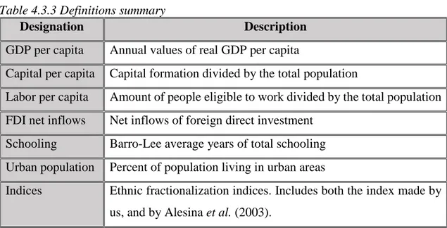
Table 4.3.3 Definitions summary
Designation Description
GDP per capita Annual values of real GDP per capita
Capital per capita Capital formation divided by the total population
Labor per capita Amount of people eligible to work divided by the total population FDI net inflows Net inflows of foreign direct investment
Schooling Barro-Lee average years of total schooling Urban population Percent of population living in urban areas
Indices Ethnic fractionalization indices. Includes both the index made by us, and by Alesina et al. (2003).
In addition to the above, Appendix I summarizes the two indices of diversity for every country, the sources used, and the years in which the sources compiled the data.
1 ”Period” column shows the years sources compiled the data which is used for index calculation.
4.4 Descriptive statistics2
Table 4.4.1 Descriptive statistics
Variable Obs Mean Std.
Dev.
Min Max Skewness
GDPpc 2584 13952.41 19666.44 193.87 144246.4 2.1643
CapitalPC 1973 3385.02 4651.59 0.0000 29576.42 2.1265
LaborPC 2427 0.4381 0.0876 0.1978 0.7545 -0.1836
FDI 2319 9.98e+09 3.71e+10 -2.90e+10 7.22e+11 8.2243
Schooling 1872 7.5600 3.0971 1.110 13.130 -0.2288
UrbanPop 2791 57.739 24.556 8.445 100.00 -0.0275
UPD_Index 2665 0.429 0.2851 0.000 0.9355 0.0379
Ethnic_AL 2665 0.402 0.2743 0.000 0.9302 0.0595
The main bit of information we can see from descriptive statistics is the extent to which the panel is unbalanced. However, this is not a major issue since the observations are missing at random. Another interesting indicator is the extreme maximum value of GDP per capita at $144 246. This outlier belongs to Monaco and is the only observation for this country in the entire dataset. Only complete observations where the cross-section is observed across the entire time-period are included in the estimation, meaning that this outlier cannot create problems in the results.
From the Table 4.4.1 we can also see that GDP per capita, capital per capita and FDI net inflows are right skewed. Hence, those variables are transformed to logarithmic form to bring them closer to a normal distribution.
Concerning the indices. By comparing the updated index with the index provided by Alesina et al. (2003) we can now see from the mean value of the updated index that indeed the world on aggregate became more diverse by approximately 0.027, or by 2.7%. This supports our expectation that diversity has increased since 1960-1980s. The difference between the two indices is not large, as Alesina et al. (2003) argued, the change in ethnic composition of societies is largely a slow process. Therefore, it makes sense that the index has not changed too much. Since the missing values from both the updated index and the indices of Alesina et al. (2003) match the already missing values from The World Bank,
their indices can be said to be available for all the countries actually included in the estimation. Thus, both indices have effectively no missing observations.
4.5 Correlation matrix
Table A.1 in Appendix II contains the correlation matrix for all the variables. We can already see that logged Capital per capita is a problematic variable for two reasons. First, it is almost perfectly correlated with the dependent variable, logged GDP per capita. This presents a problem as they essentially explain the same economic outcome. Second, it has very high (above 0.70) correlation with three other control variables, logged FDI (lnFDI), Schooling and Urban Population, therefore it also presents a problem of multicollinearity. We are not dropping it just yet however, as we want to see the variance inflation factors first and drop variables based on those. The negative correlations between the indices of diversity and GDP per capita are also evident.
4.6 Assumptions
Even though the data for the calculation of the indices is collected at various years, the index itself is calculated only once. In our case the data was collected from 2000 to 2017 and the index was calculated in 2018. In order to use the index in a dataset with other years and not only 2018, the assumption that the index is time-invariant has to be made. This assumption can be supported with the argument that changing a country’s ethnic diversity composition is a difficult task in a timeframe of 13 years, short of drastic events such as genocide or mass displacements (Alesina et al. 2003).
4.7 Model selection
The model selection process involves choosing between the available models to find which one is the preferred choice for the data at our disposal. We test three models commonly used with panel data, Pooled OLS regression, Random effects model (REM), and a Fixed effects model (FEM). The test results are discussed in the following paragraphs and the outputs of the tests can be found in Appendix II.
Breusch-Pagan LM test is used to distinguish between Pooled and REM. The test results say that we should use a random effects model. The large sample size (N=217) with a
short timeframe (T=13) also speaks in favor of the random effects model (Gujarati & Porter, 2009). However, to be objective it is also necessary to test between a fixed effects model and a random effects model to be sure that random effects is indeed the only preferred choice. A Hausman test can distinguish between the two models. Under the null hypothesis a RE model is preferred, whereas under alternative the FE model is preferred. The results of the test indicate that the fixed effects model is preferred over a random effects model.
Not only is a FE model backed by the Hausman test, this model would also be useful to account for individual differences between countries, an advantage, for example a Pooled OLS regression does not provide. However, it cannot be used because we have time-invariant variables, and a fixed effects model cannot estimate coefficients for such variables. Because of this reason a FEM is not an option even as a robustness check for only our control variables, since one of them (Schooling) is also time-invariant.
We arrive at a conclusion that we need a model that takes into account the fixed effect assumption that the individual-specific effects are correlated with the independent variables and at the same time allows for time-invariant variables to be present in the model. Hausman-Taylor model meets all of the above criteria.
4.8 Estimated model
The estimated model can be expressed as:
𝑙𝑛𝑌𝑖𝑡 = 𝑇𝑡𝛽1+ 𝑙𝑛𝐾𝑖𝑡𝛽2+ 𝛬𝑖𝑡𝛽3+ 𝑙𝑛𝛷𝑖𝑡𝛽4+ 𝑋𝑖𝑎1+ 𝑅𝑖𝑎2+ 𝛤𝑖𝑎3+ 𝛩𝑖𝑎4+ 𝜀𝑖𝑡+ 𝜇𝑖𝑡 Where:
Designation Variable
Dependent
lnYit Log of GDP per capita
Independent
Tt Time dummies
lnKit Log of Capital per capita
Λit Labor per capita
lnΦit Log of FDI net inflows
Xi Variable of interest (index)
Γi Average years of schooling
ε
it Error termµ
it Unobserved random effectWhere also:
•
Tt is assumed to be time-varying and uncorrelated withµ
it•
Xi and Ri are assumed to be time-invariant and uncorrelated withµ
it•
lnKit, Λit, lnΦit are assumed to be time-varying and correlated withµ
it•
Γi and Θi are assumed to be time-invariant and correlated withµ
itHence:
•
Tt is said to be time-varying and exogenous within the model•
Xi and Ri are said to be time-invariant and exogenous within the model•
lnKit, Λit, lnΦit are said to be time-varying and endogenous within the model•
Γit and Θi are said to be time-invariant and endogenous within the modelTo explain the above. The Hausman-Taylor (HT) model classifies variables by using two dimensions. First, whether a variable is time-varying or time-invariant, and second, whether the variable is correlated with the individual-specific unobserved random effect (hence, endogenous), or uncorrelated with the individual-specific unobserved random effect (hence, exogenous).
The assumption that only some of the regressors are exogenous and others endogenous is both stronger than that of a REM, which assumes complete exogeneity of the regressors, and stronger than that of FEM, which assumes complete endogeneity of the regressors. In addition, exogenous variables in HT are assumed to affect the endogenous ones, but not vice-versa. For example, ethnic diversity (exogenous variable) affects capital (endogenous variable), and capital in turn affects GDP growth. But ethnic diversity is assumed to be unaffected by any other variables in the system.
In the equation above we have already specified which variables are assumed to be endogenous and which exogenous, but what is the reasoning behind the assumption that for example, capital is endogenous. Designating variables as endogenous or exogenous is not as a clear-cut process. The same variable can be either endogenous or exogenous dependent on model specification, which other variables are included, what the dependent variable is, or what the research question is, among others. In addition, it is very difficult to statistically prove definite endogeneity or exogeneity of a particular variable. Our chosen way of identifying variables as endogenous or exogenous is reverse causality. It makes intuitive sense that for example, income (or output) is affected by the amount of capital, but the more income one has, the more capital they can acquire. If income is a dependent variable and capital is an independent one, then there is reverse causality between them and it is said that “endogeneity is caused by reverse causality”, hence capital is an endogenous independent variable in this example.
Using reverse causality, we can then support the assumptions of endogeneity and exogeneity in a Hausman-Taylor model outlined in the beginning of this section. Note that the variables described next are assumed to be endogenous or exogenous only within the framework of our model and our timeframe. This section is not intended to make general statements about definite endogeneity or exogeneity of particular variables.
Hence:
Time dummies (Tt): are assumed to be time-varying and exogenous within the model, because time is time-varying and is one of the variables that are always exogenous, because nothing affects the passage of time.
Diversity indices (Xi): if using reverse causality as reasoning for endogeneity, then the diversity indices can be endogenous. Because for example, richer countries attract more immigrants. However, we assume it to be exogenous within our model for the following reason. If it is designated as endogenous, this results in the control variables acting erratically, they change signs to the incorrect ones, as well as lose significance. Therefore, we know that it is correct for the indices of ethnic diversity to be exogenous within the framework of our model, but we do not know why it is the case.
Capital (lnKit): is assumed to be endogenous within the model. When looking at reverse causality as a cause of endogeneity Capital is perhaps the most endogenous variable in our equation. The example given previously about the relationship of capital with income (GDP per capita), whereas the more income one has the more capital they can acquire supports reverse causality if GDP is the dependent variable and capital is a regressor. Moreover, the correlation matrix described in descriptive statistics section shows that the correlation between GDP per capita and Capital is very high3, meaning that the two variables are very similar. Correlation does not imply causality but, shows that the two variables go hand in hand.
Labor (Λit): is assumed to be endogenous. Labor might exhibit reverse causality with GDP per capita because of the following reason. Say labor increases, then output should increase, however the more output is produced the more workplaces might become available because the economy is booming. Hence, we assume labor in terms of workplaces is endogenously determined within the model.
FDI (lnΦit): is assumed to be endogenous. Schneider & Frey (1985) show that the higher real per capita GNP is, the higher is the level of foreign direct investment. In other words, they have found that gross national product is the determinant of foreign direct investment. Therefore, if FDI is an independent variable and GDP per capita is the dependent, we can say that there is reverse causality, hence FDI is endogenous within the model.
Schooling (Γit): is assumed to be endogenous. Even though it is time-invariant and hence can be specified as exogenous, we will assume schooling to be endogenous for the following reason. In general people in more economically developed countries are more likely to enroll in tertiary education (The World Bank, Task Force on Higher Education in Developing Countries, 2000). This means that economic success is the determinant of schooling. Meaning not only Schooling affects GDP per capita, but GDP per capita also affects schooling. Therefore, there is a reverse causality relationship between them, therefore Schooling is endogenous.
Every regression will be run using the above estimated model, only the Xi (index) variable will change and every subsequent estimated model equation will specify which index was used.
Additionally, Capital per capita is removed from the model for subsequent estimations due to high multicollinearity, its VIF>5 (Craney & Surles, 2002). (see Figure 2 in Appendix III). The model is run using robust standard errors.
5 Results
5.1 Updated Ethnic Fractionalization
The estimated model for updated ethnic fractionalization can be expressed as:
𝑙𝑛𝑌𝑖𝑡 = 𝑇𝑡𝛽1+ 𝑙𝑛𝐾𝑖𝑡𝛽2+ 𝛬𝑖𝑡𝛽3+ 𝑙𝑛𝛷𝑖𝑡𝛽4+ 𝑋𝑖𝑎1+ 𝑅𝑖𝑎2+ 𝛤𝑖𝑎3+ 𝛩𝑖𝑎4+ 𝜀𝑖𝑡+ 𝜇𝑖𝑡 Where:
Designation Variable
Dependent
lnYit Log of GDP per capita
Independent
Tt Time dummies
Λit Labor per capita
lnΦit Log of FDI net inflows
Xi Updated ethnic fractionalization index
Ri Regional dummies
Γit Average years of schooling
ε
it Error termµ
it Unobserved random effectResult:
Variable Coef. (p-value)
TVexogenous Y2003 -0.2330 (0.000) Y2004 -0.1982 (0.000) Y2005 -0.1783 (0.000) Y2006 -0.1452 (0.000) Y2007 -0.1160 (0.000) Y2008 -0.0945 (0.000) Y2009 -0.1075 (0.000) Y2010 -0.0887 (0.000) Y2011 -0.0685 (0.000) Y2012 -0.0486 (0.000) Y2013 -0.0304 (0.003) Y2014 -0.0150 (0.140) TVendogenous LaborPC 0.4956 (0.002) UrbanPop 0.0078 (0.000) lnFDI 0.0098 (0.000)
TIexogenous UPD_Index -0.3658 (0.264) R_AmCaribbean 0.2078 (0.641) R_EASPacific 0.2093 (0.570) R_EurCA 0.2241 (0.752) R_MENA 0.9774 (0.007) TIendogenous Schooling 0.3122 (0.007) constant 5.4655 (0.000) p-values in parentheses TVexogenous=time-varying exogenous; TVendogenous=time-varying endogenous; TIexogenous=time-invariant exogenous; TIendogenous=time-invariant endogenous;
5.2 Ethnic fractionalization (Alesina et al. 2003)
The estimated model for ethnic fractionalization could be written as:
𝑙𝑛𝑌𝑖𝑡 = 𝑇𝑡𝛽1+ 𝑙𝑛𝐾𝑖𝑡𝛽2+ 𝛬𝑖𝑡𝛽3+ 𝑙𝑛𝛷𝑖𝑡𝛽4+ 𝑋𝑖𝑎1+ 𝑅𝑖𝑎2+ 𝛤𝑖𝑎3+ 𝛩𝑖𝑎4+ 𝜀𝑖𝑡+ 𝜇𝑖𝑡 Where:
Designation Variable
Dependent
lnYit Log of GDP per capita
Independent
Tt Time dummies
Λit Labor per capita
lnΦit Log of FDI net inflows
Xi Ethnic fractionalization (Alesina et al. 2003)
Ri Regional dummies
Γit Average years of schooling
ε
it Error termResult:
Variable Coef. (p-value)
TVexogenous Y2003 -0.2327 (0.000) Y2004 -0.1981 (0.000) Y2005 -0.1781 (0.000) Y2006 -0.1450 (0.000) Y2007 -0.1159 (0.000) Y2008 -0.0944 (0.000) Y2009 -0.1074 (0.000) Y2010 -0.0886 (0.000) Y2011 -0.0684 (0.000) Y2012 -0.0486 (0.000) Y2013 -0.0304 (0.003) Y2014 -0.0150 (0.141) TVendogenous LaborPC 0.4950 (0.002) UrbanPop 0.0079 (0.000) lnFDI 0.0098 (0.000) TIexogenous Ethnic_Alesina -0.9774 (0.003) R_AmCaribbean 0.1070 (0.808) R_EASPacific 0.0284 (0.938) R_EurCA 0.0492 (0.944) R_MENA 0.8168 (0.022) TIendogenous Schooling 0.3031 (0.008) constant 5.9004 (0.000) p-values in parentheses TVexogenous=time-varying exogenous; TVendogenous=time-varying endogenous; TIexogenous=time-invariant exogenous; TIendogenous=time-invariant endogenous;
5.3 Interpretation
The interpretation of the Alesina et al. (2003) ethnicity index is the following. If the probability that two randomly selected individuals are not of the same ethnic group increases by 1 percentage point, then GDP per capita decreases by approximately 0.98%, ceteris paribus (0.01 × (−0.98) × 100% ). One standard deviation in ethnic fractionalization (0.26) therefore brings GDP per capita down on average by 25%. Standard deviation for the natural logarithm of GDP per capita is 1.52, or 𝑒1.52− 1 ≈ 357%, so we can say that change Alesina’s index explains 25
357 ≈ 7% of the variation in GDP per capita. This number looks correct and is comparable in magnitude with the original study.
While original index by Alesina et al. (2003) is significant, its modified version presented in Section 5.1 is not. Despite the expected negative sign, both magnitude and statistical significance are markedly lower.
6 Analysis
Two key findings emerge from our study. First, is that the world on aggregate has become more diverse. Second, when we update the index of ethnic diversity with more recent data, it is insignificant, while preserving a negative sign. This in turn implies that ethnic diversity has become an insignificant factor in determining economic growth in comparison to the decades examined by Alesina et al. (2003)4. In turn, when ethnic fractionalization index in the original version by Alesina et al. (2003) enters our equation, it appears to negatively affect GDP per capita.
The magnitudes for all the coefficients are realistic, so we have a puzzle to explain. How come that when updated, fractionalization index loses its statistical significance on the same dataset? When using the index provided by Alesina et al. (2003) in our model, it gives the expected negative coefficient that is significant, just as in their original study. This gives us a reason to believe that the insignificance of our updated index is indeed the correct outcome. We argue that hints of a possible explanation lie in the channels through which ethnic diversity affects growth. Increases in the positive channels could balance-out the already present negative channels, therefore removing a clear negative role of ethnic diversity in economic growth.
One of the positive channels is social trust, otherwise called generalised trust. According to Dincer (2011) there is a U-shaped relationship between trust and ethnic fractionalization, where trust is minimised at index value of 0.34, after which more diversity induces more trust. Ethnic fractionalization index by Alesina et al. (2003) averages at 0.402 for the entire world. Whereas our updated index equals 0.429 on average for the same sample of countries. This implies that the world on aggregate has become more diverse by approximately 2.7%, but more importantly moved further away from the minimising value of 0.34, meaning that trust on aggregate has also increased. Trust in turn, has a positive effect on economic growth as outlined in the theory section. This is a positive change of the effect of ethnic diversity on economic growth through an increase in trust.
Another positive channel is misallocation of labor. Immigration has increased since the time-period considered by Alesina et al. (2003) and societies have become more diverse (Castles, 2013). The last is also evident from the mean value of the indices (see descriptive statistics). Therefore, the labor markets have become more saturated in terms of talents, skills and work experiences. This means that the misallocation of labor decreased because every employer in the economy has now more opportunities to hire those workers that fit his/her job in the best possible way. The reduced misallocation of labor is associated with increased level of total factor productivity and ultimately contributes to economic growth (Restuccia & Rogerson, 2008; Hsieh & Klenow, 2009).
The insignificance of ethnic diversity could also be credited to a decrease in the negative channels. However, this is not the case with at least conflict. As outlined in the theory section, high levels of ethnic diversity have been linked with increased incidence of civil conflict. We have found that the world has become on average more diverse, and when looking at the graph in Appendix IV we can see that the number of civil wars has been increasing substantially since 1960s. It is safe to say that some portion of those conflicts is based on ethnic grounds, therefore, the negative effect of ethnic diversity on economic growth through conflict has not vanished and may have become even more severe if one is to calculate the portion of civil conflicts that are based on ethnicity.
We want to give special attention to the fact that channels described in our analysis, such as conflict, trust and misallocation of labor, are not the only ones that have affected our result. There are a lot of other channels which link ethnic diversity and GDP per capita growth. The main goal of this paper is to find the effect of ethnic diversity on economic growth, and not to find how ethnic diversity affects GDP per capita growth through a certain channel/channels. Therefore, in our case, channels such as trust, misallocation of labor and conflict act as examples to show how ethnic diversity may be linked with GDP per capita growth. The negative impact of ethnic diversity on economic growth through conflict (and other negative channels that are not included in our paper) could have increased since the decades investigated by Alesina et al. (2003). However, we can also argue that the positive impact of ethnic diversity on economic growth through such channels as misallocation of labor, trust (and other positive channels that are not included in our paper) could have increased as well. In the end however, particularly in the framework of our research question it does not matter which channels have led to a
positive or negative impact of ethnic diversity on GDP per capita growth and what was the magnitude of a particular channel’s influence. We only need to focus on the fact that somehow the positive effects of ethnic diversity on economic growth balanced-out the negative ones which resulted in insignificance.
To sum up, increased ethnic fractionalization affects economic growth both positively and negatively depending on the channel connecting these variables. We argue that the negative result previously achieved by Alesina et al. (2003) holds and may have become even stronger, however on aggregate the increases in positive channels create a balancing-out effect, hence there is no longer a clear negative relationship between ethnic diversity and economic growth. This results in an insignificant coefficient for the updated index and leads to a conclusion that ethnic diversity indeed plays no significant role in determining economic growth during the time-period under our investigation. Since the effect of ethnic fractionalization on growth is composed of channels that act in opposite directions, its final identification is a task for future research.
7 Limitations
The main limitation of this thesis lies in the measurement of the indices, which itself comes from the definitions of what an ethnic group is. To explain, since we use the index of Alesina et al. (2003) as a benchmark for our updated index, the techniques of index calculation should be identical to theirs in order to be able to directly compare the results achieved by the two indices. This implies that both the criteria of separating the population of a country into ethnic groups and the sources used should have been the same. Alesina et al. (2003) used data form three different sources and then cross-checked the index calculated from those sources to be identical up to three decimal places. Even though the majority of our data on ethnic groups is collected from Encyclopaedia Britannica just as Alesina et al. (2003) is, we do not do the cross-checking procedure and instead take the data from Encyclopaedia Britannica even if it is also available from other sources. This results in some discrepancies in the calculated values of our updated index in comparison to Alesina et al. (2003) index. Therefore, the change in results of ethnic diversity from negative to insignificant may be caused by the measurement differences of ethnic fractionalization between our paper and Alesina et al. (2003).
Our model also leaves out other important types of observable diversity, with examples such as age or gender. It also leaves out unobservable diversity, such as personal abilities or knowledge gained outside of educational system. Inclusion of these types in the calculation of diversity indices or at least some degree of control for them could yield different results. One could also control for a common international language such as a proportion of English speakers as a secondary language in a country. With different ethnicity often comes a different language, and positive effects of for example, misallocation of labor could be dampened because a person cannot contribute their talents and abilities fully without language.
8 Conclusion
This paper analyzes the role ethnic diversity plays in determining economic growth in terms of real GDP per capita during the period of 2003-2015. The first part of the paper examines the theoretical reasoning behind why ethnic diversity may positively or negatively affect growth while also covering previous research on this topic. Ethnic diversity is measured by a fractionalization index calculated by the authors using the most recent data on ethnic groups available. Another index of ethnic fractionalization by Alesina et al. (2003) was used as a robustness check and to give insights as to what changes occurred in the relationship of ethnic diversity and economic growth. We use a panel approach for a dataset of 217 countries for 13 years and employ a Hausman-Taylor model for estimation.
Our findings suggest that the role of ethnic diversity in influencing economic growth has changed since the time period investigated by Alesina et al. (2003). We argue that this change has been brought about by the increase in positive channels of for example, reduced misallocation and increased levels of societal trust. Resulting in them balancing out the negative channels such as conflict, poor administration, provision of public goods and special interest politics among others. This balance in turn results in the updated index of ethnic diversity to be statistically insignificant since there is no more a clear negative or positive effect of ethnic diversity on growth.
One route for further research would be to attempt to disentangle the positive and negative channels. It is also interesting to see if the positive effects explored in this paper will continue to grow stronger and eventually outweigh the negative ones, resulting in an aggregate positive and statistically significant effect of ethnic diversity on economic growth in the future.
9 Reference list
Abadie, A., & Gardeazabal, J. (2003). The Economic Costs of Conflict: A Case Study of the Basque Country. American Economic Review, 93 (1), 113-132. doi: 10.1257/000282803321455188 Ager, P., & Brückner, M. (2013). Cultural diversity and economic growth: Evidence from the US during the age of mass migration. European Economic Review, 64, 76-97.
https://doi.org/10.1016/j.euroecorev.2013.07.011
Alesina, A., Baqir, R., & Easterly, W. (1999). Public goods and ethnic divisions. The Quarterly
Journal of Economics, 114(4), 1243-1284.https://doi.org/10.1162/003355399556269
Alesina, A., Devleeschauwer, A., Easterly, W., Kurlat, S., & Wacziarg, R. (2003). Fractionalization. Journal of Economic Growth, 8 (2), 155-194.
https://doi.org/10.1023/A:1024471506938
Alesina, A., Harnoss, J., & Rapoport, H. (2016). Birthplace diversity and economic prosperity.
Journal of Economic Growth, 21(2), 101-138.doi: 10.1007/s10887-016-9127-6
Ashraf, Q., & Galor, O. (2011). Cultural Diversity, Geographical Isolation, and the Origin of
the Wealth of Nations (Working Paper No. 17640). Retrieved from the National Bureau of
Economic Research: http://www.nber.org/papers/w17640
Barro, R.G. (1991). Economic Growth in a Cross Section of Countries. The Quarterly Journal of
Economics, 106 (2), 407-443. https://doi.org/10.2307/2937943
Barro, R. J., & Martin, S. I. X., (2004). Economic Growth. The MIT Press.
Barro, R. J., & Lee, J. W. (2013). A new data set of educational attainment in the world, 1950– 2010. Journal of development economics, 104, 184-198.
https://doi.org/10.1016/j.jdeveco.2012.10.001
Benhabib, J., & Spiegel, M. M. (2005). Human capital and technology diffusion. Handbook of
economic growth, 1, 935-966. https://doi.org/10.1016/S1574-0684(05)01013-0
Bove, V., & Elia, L. (2016). Migration, Diversity, and Economic Growth. World Development,
89, 227-239. https://doi.org/10.1016/j.worlddev.2016.08.012
Bloom, D.E., Canning, D., & Fink, G. (2008). Urbanization and the Wealth of Nations. Science,
Borensztein, E., De Gregorio, J., & Lee, J. W. (1998). How does foreign direct investment affect economic growth?. Journal of international Economics, 45(1), 115-135.
https://doi.org/10.1016/S0022-1996(97)00033-0
Bossert, W., D’Ambrosio, C., & La Ferrara, E. (2011). A Generalized Index of Fractionalization.
Economica, 78 (312), 723-750. https://doi.org/10.1111/j.1468-0335.2010.00844.x
Castles, S., de Haas, H., & Miller, M.J. (2013). The Age of Migration: International Population
Movements in the Modern World. Hampshire, UK: Palgrave Macmillan.
Cederman, L., & Girardin, L. (2007). Beyond Fractionalization: Mapping Ethnicity onto Nationalist Insurgencies. American Political Science Review, 101(1), 173-185. doi: 10.1017/S0003055407070086
Collier, P. (2000). Economic Causes of Civil Conflict and their Implications for Policy. Informally published manuscript. Retrieved from
http://citeseerx.ist.psu.edu/viewdoc/summary?doi=10.1.1.460.9440
Collier, P., Hoeffler, A., & Söderbom, M. (2004). On the Duration of Civil War. Journal of Peace
Research, 41 (3), 253-273. https://doi.org/10.1177/0022343304043769
Collier, P. (2013). Exodus: How migration is changing our world. Oxford: Oxford University Press.
Craney, T.A., & Surles, J.G. (2002). Model-Dependent Variance Inflation Factor Cutoff Values.
Quality Engineering, 14 (3), 391-403. doi: 10.1081/QEN-120001878
Dincer, O.C. & Uslaner, E.M. (2009). Trust and growth. Public Choice, 142 (59), 59–67. https://doi.org/10.1007/s11127-009-9473-4
Dincer, O. C. (2011). Ethnic diversity and trust. Contemporary Economic Policy, 29 (2), 284-293. https://doi.org/10.1111/j.1465-7287.2010.00215.x
Easterly, W., & Levine, R. (1997). Africa's Growth Tragedy: Policies and Ethnic Divisions. The
Quarterly Journal of Economics, 112 (4), 1203-1250. https://doi.org/10.1162/003355300555466
Fearon, J.D. (2003). Ethnic and Cultural Diversity by Country. Journal of Economic Growth,
8(2), 195-222. Retrieved from https://link.springer.com/article/10.1023/A:1024419522867
Fearon J.D. (2004). Why Do Some Civil Wars Last So Much Longer than Others? Journal of Peace