Tracking techniques for automotive virtual reality

Björn Blissing

Tracking techniques for

automotive virtual reality

VTI notat 25A-2016

|

T

racking techniques for automotiv

www.vti.se/en/publications

VTI notat 25A-2016

Published 2016

VTI notat 25A-2016

Tracking techniques

for automotive virtual reality

Diarienr: 2012/0511-25 Omslagsbild: Karin Linhardt Tryck: LiU-tryck, Linköping 2016

Preface

This work has been carried out at VTI and has been financed by internal funding. Linköping, september 2016

Quality review

Internal peer review was performed on 7 September 2016 by Camilla Ekström. Björn Blissing has made alterations to the final manuscript of the report. The research director Arne Nåbo examined and approved the report for publication on 25 October 2016. The conclusions and recommendations expressed are the author’s and do not necessarily reflect VTI’s opinion as an authority.

Kvalitetsgranskning

Intern peer review har genomförts 7 september 2016 av Camilla Ekström. Björn Blissing har genomfört justeringar av slutligt rapportmanus. Forskningschef Arne Nåbo har därefter granskat och godkänt publikationen för publicering 25 oktober 2016. De slutsatser och rekommendationer som uttrycks är författarens egna och speglar inte nödvändigtvis myndigheten VTI:s uppfattning.

Contents

2.2.1. Example of scene motion . . . 15

2.3. Tracking artifacts . . . 16

2.3.1. Static errors . . . 16

2.3.2. Dynamic errors . . . 16

3. General principles of tracking . . . . 17

3.1. Dead reckoning . . . 17 3.2. Trilateration . . . 17 3.3. Triangulation . . . 20 4. Tracking Techniques . . . . 22 4.1. Mechanical trackers . . . 22 4.2. Acoustical trackers . . . 22 4.3. Electromagnetic trackers . . . 22 4.4. Inertial trackers . . . 23 4.5. Optical trackers . . . 23 4.6. Video trackers . . . 24 4.7. Hybrid trackers . . . 24

4.8. Full body tracking . . . 25

5. Tracking for Automotive Virtual Reality Applications . . . . 26

5.1. Tracking the vehicle . . . 26

5.2. Tracking inside the vehicle . . . 27

6. Conclusions . . . . 28

Summary

Tracking techniques for automotive virtual reality – A review

by Björn Blissing (VTI)

This publication is a review of available technologies for tracking the user in virtual reality systems. Tracking the user location is important for generating views that adapts to the user’s movements. This review begins with the basic terms used in virtual reality in general. Followed by the important characteristics for tracking equipment. This is followed by a chapter on the fundamental algorithms used for position calculations. Then the most common technologies with their advantages and disadvantages are presented. The text conclude with how these technologies are used in automotive virtual reality.

Sammanfattning

Spårningstekniker för fordonsbaserad virtuell verklighet – En kunskapsöversikt

av Björn Blissing (VTI)

Denna publikation är en sammanställning av den teknologi som används i virtuell verklighet för att spåra användaren. Att spåra var användaren befinner sig är viktigt för att alstra vyer som anpassar sig till användarens rörelser.

Publikationen inleds med de grundläggande termer som används inom virtuell verklighet i allmänhet. Därefter presenteras viktiga egenskaper för spårningsutrustning. Detta följs av ett kapitel om de grundläggande algoritmer som används för att beräkna positioner. Sedan presenteras de vanligaste teknologierna för spårning med deras för- och nackdelar. Texten avslutas med hur dessa teknologier används inom fordonsbaserad virtuell verklighet.

1.

Introduction

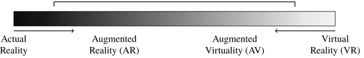
Virtual reality (VR) is meant to immerse the user in a computer simulation, generating an oriented view in respect to the user (Bishop and Fuchs, 1992). There is also steps between the real world and being in a totally virtual world, which has been described by Milgram et al. (1994) as the Reality-Virtuality

Continuum(See figure 1). Everything between the two extremes in this continuum is known as Mixed

Reality (MR). Augmented Reality (AR) is when the virtual objects or annotations have been added to

the view of the real world, while Augmented Virtuality (AV) is when real world objects are brought into an otherwise virtual world. To be able to achieve any of these types of VR experiences some form of tracking is needed.

The requirements for the tracking system depends on the selected display technology. The three most common display technology categories are:

Fixed Displays — Displays fixed to a static position relative to the user of the system. Starting with a

computer monitor with an oriented view, so called fish tank VR (Ware et al., 1993) — up to large room sized six-sided back projected spaces, known as CAVEs (Cruz-Neira et al., 1993).

Handheld Displays — Mobile phones or tablets can be used for virtual reality experiences.

Most modern devices are already equipped with sensors which can be used for tracking. Especially AR solutions have been common for these types of devices.

Head Mounted Displays — Wearable displays which enables the users to be completely immersed in

to the virtual world. These usually feature two displays, one for each eye, providing stereoscopic views. Head Mounted Displays (HMD) comes in three main categories; Opaque HMDs for pure virtual reality, Optical see-through HMDs and Video see-through HMDs for mixed reality. The tracking requirements for VR-solution based on fixed screens the requirements are less strict than for handheld or head mounted displays used for MR. This is due to the fact that in MR the user can use the real world as reference, which in turn makes tracking artifacts easier to detect.

The user of the virtual world may not be the only thing that is desired to be tracked. Tracking technologies can also be used to position and orient tools used in the virtual worlds; such as wands, styluses and 3D mice.

Actual

Reality Reality (AR)Augmented Virtuality (AV)Augmented Reality (VR)Virtual Mixed Reality (MR)

Figure 1. The Reality-Virtuality Continuum as suggested by Milgram et al. (1994).

1.1.

Previous surveys

There is a lack of modern surveys regarding tracking technologies. The survey by Ferrin (1991) is focused on helmet tracking technologies mainly for military use. Then there are surveys on tracking technologies for virtual reality, which focuses on the working principles and the different performance of individual systems such as the survey by Bhatnagar (1993) as well as a similar survey by Rolland et al. (2001).

2.

Tracking metrics

When comparing tracking systems there are some different metrics that can be important to consider depending on the desired application.

Update rate How often measurements are performed and reported.

Input delay The time from change of sensor position until a new measurement is reported. This is

sometimes called Lag or Latency. (See section 2.2 for a detailed description.)

Precision How spread repeated measurements of a stationary target are. Accuracy The difference between the true value and the measured value. Resolution The smallest change in position or orientation that can be measured.

Absolute/Relative If the tracker reports measurements in absolute coordinates or as relative changes Working Volume The volume within the tracker can report data

Degrees of freedom How many degrees of freedom the tracker is able to measure. (See section 2.1 for

a detailed description.)

Environmental robustness How robust the tracker is for the environment it is supposed to work in, i.e

tolerance for temperature, humidity, noise, lighting conditions etc.

Ergonomics The weight and physical dimensions of the sensors. Do the tracker restrict movement in

any way, for example due to wires, mechanical limits or gimbal lock situations(See section 4.1). It can also be important to know if the tracker can handle occlusion problems (line of sight) and if multiple trackers are possible to use within the same tracking volume.

2.1.

Degrees of freedom

In our physical world we move about in six degrees of freedom (DOF). These are translatory motion in three axis and rotational motion around these axis. The linear motion are sometimes denoted Sway(x), Surge(y) and Heave (z), while the rotational motions are denoted Pitch(θ), Roll(ϕ) and Yaw(ψ). A tracking system which only tracks rotations would be classified as a 3-DOF system. A tracking system which only tracks translations would also be a 3-DOF system (see figure 2a), while a system capable of track both translations and orientation would be a 6-DOF system (see figure 2b).

x

y

z

(a) 3-DOF point

x

y

z

ψ

θ

ϕ

Figure 2. Some tracking technology only tracks in 3-DOF, while others can track points in 6-DOF.

x₁ y₁ z1 x₂ y2 z₂ ψ ϕ

(a) A 5-DOF system using two 3-DOF points

x₁ y₁ z1 x₂ y2 z₂ x3 y₃ z3 ψ θ ϕ

(b) A 6-DOF system using three 3-DOF points

Figure 3. Connecting points to gain more degrees of freedom.

Due to the fact that some tracking technology are only tracking translations the rotational information must be extracted in other ways. One way is to interlink multiple 3-DOF points. Rotations can be calculated by combining information from tracking translation of multiple static linked points. By connecting two 3-DOF points with a rigid rod the coupled system will achieve 5-DOF (see figure 3a). If three 3-DOF point are coupled the system will have 6-DOF. At least 3 orthogonal points needs to be tracked in space in order to calculate the orientation around all axes (see figure 3b). Even though 6-DOF is sufficient to describe all motions in our three dimensional world you will sometime see tracking systems which are specified with a higher number of DOF. This usually means that the system tracks multiple things at the time. For example a system which tracks an arm. Such a system could be specified as a 9-DOF system because it consists of a 6-DOF tracker positioned at the hand and a 3-DOF system at the elbow. Another example of higher DOF system could be a system which consists of multiple tracking technologies which have different tracking volumes or accuracy. For example a system specified as 8-DOF could be consisting of a 6-DOF tracker for small scale tracking coupled with a 2-DOF tracker for large scale tracking.

2.2.

Input delay

Input delay is the time delay from tracker input until the corresponding measurement have reached the the destination. For VR-systems the destination is when graphics are shown to the user. This includes both the delay in the tracking system as well as the delay in the visual presentation. This type of delay is sometimes called input latency or motion-to-photon latency. Uncompensated latency can have the effect on the user that static environments appear to move when turning their head, i.e. scene motion. It is therefore very important to keep the latency to a minimum, although some latency compensation can be achieved by using motion prediction (Azuma and Bishop, 1995).

2.2.1. Example of scene motion

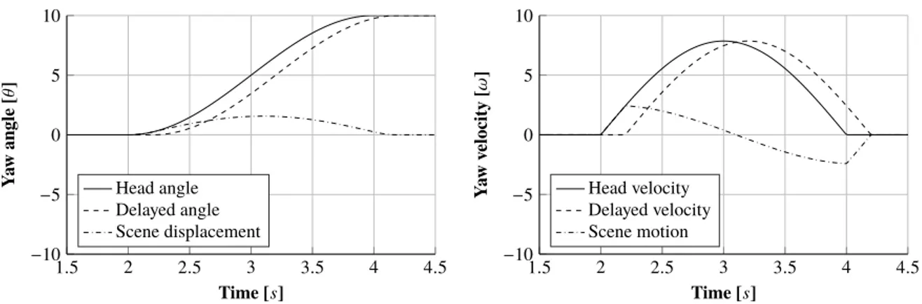
Figure 4 show a simulation of the effects of 100ms latency on a headturn from 0° to 10° with a duration of 2 seconds. In the beginning the head turns without the corresponding movement in the HMD leading to scene displacement. The initial acceleration of the head leads to the scene starts moving with the head, i.e. positive scene velocity. The velocity of the head peaks in the center of the head turn and shortly after the scene velocity starts becomes negative and the scene starts to move against the direction of the head turn, i.e. negative scene velocity. Jerald et al. (2008) have shown that subjects are

1.5 2 2.5 3 3.5 4 4.5 −10 −5 0 5 10 Time [s] Y a w angle [θ ] Head angle Delayed angle Scene displacement 1.5 2 2.5 3 3.5 4 4.5 −10 −5 0 5 10 Time [s] Y a w v elocity [ω ] Head velocity Delayed velocity Scene motion

Figure 4. Visualizing head motion and scene motion.

2.3.

Tracking artifacts

Any errors in tracking can break presence and cause simulator sickness (Drascic and Milgram, 1996; Kruijff et al., 2010). There exist several types of tracking artifacts which may constrain the desired performance. These can be divided into two classes; Static- and dynamic artifacts.

2.3.1. Static errors

Spatial Distortion Static errors within the tracking volume in regards of reported position, orientation

and/or scale. The magnitude of these may differ within the tracking volume, but could be compensated for by using a mapping function.

Jitter Noise in the tracker data causing the reported position and orientation to shake, even though the

tracker is actually still. According to Foxlin (2002) jitter of 0.05° r.m.s. in orientation and 1 mm r.m.s. in position is generally unnoticeable.

Drift Variation in tracker output to slow to observe as motion, which still could make the tracker

output drift from the correct position and/or orientation. To compensate for drift, periodic absolute tracker measurements are needed as correction.

2.3.2. Dynamic errors

Latency The delay of the signal which causes the reported measurement to lag behind the correct

value. (See section 2.2)

Latency Jitter Variation of latency between different tracker measurements, which will cause jitter

during movement. (See figure 5)

Other Error Any dynamic errors not caused by latency, for example motion prediction errors or

sensor fusion errors.

Time [s] Y a w angle [θ ] Time [s] Y a w angle [θ ]

Figure 5. The left plot shows a jitter free signal. The right plot shows a signal where a couple of measurements have been delayed, which resulting in perceived jitter.

3.

General principles of tracking

This chapter describes some common principles used in different tracking technologies.

3.1.

Dead reckoning

Given the position is know at time P0and the velocity v0the new position Ptcan be estimated by

numerical integration:

Pt ≈ P0+ v0∆t (3.1)

The difference between the real position and the estimated position can be written as the error vector ε, resulting in the following equation for the position:

P_t = P₀+ v₀· ∆t+ ε (3.2)

If the initial acceleration a0is know the equation can be written as:

Pt = P0+ v0· ∆t+

a₀· ∆t2

2 + ε (3.3)

The main drawback of dead reckoning is drift, due to integration errors. The duration until drift will become noticeable will depend on the magnitude of the error factor ε. Dead reckoning can only remain accurate during very short time periods and will drift unless complemented with some form of fixed reference tracking.

3.2.

Trilateration

Trilateration (or Multilateration) is the process of calculating the position using distances from other already known positions. To calculate a position in space at least 3 known positions are needed. Knowing the distances r1, r2and r3from our tracked position (x, y, z) to the three known position

(0, 0, 0), (d, 0, 0) and (i, j, 0) the following model using three spheres can constructed (see figure 6). The tracked position P will be where the three spheres intersect:

(0, 0, 0) i j r₁ r₂ r₃ d P

The intersection between the three spheres can be derived using the following system of equations:

r₁2= x2+ y2+ z2 (3.4)

r₂2= (x − d)2+ y2+ z2 (3.5) r₃2= (x − i)2+ (y − j)2+ z2 (3.6) Subtracting equation 3.4 and 3.5 and solve for x:

r₁2− r₂2 = (x2+ y2+ z2) − ((x − d)2+ y2+ z2) r₁2− r₂2 = x2− (x − d)2 r₁2− r₂2 = x2− (x2−2xd + d2) r₁2− r₂2 = 2xd − d2 r₁2− r₂2+ d2 = 2xd (3.7) Resulting in the x-coordinate of the point P.

x = r1

2_{− r2}2_{+ d}2

2d (3.8)

Substituting the equation for x back into the equation 3.4 produces the equation for a circle (Equation 3.9), which is the intersection of the first two spheres.

r₁2= r1 2_{− r} 22+ d2 2d !2 + y2_{+ z}2 r₁2= (r1 2_{− r2}2_{+ d}2₎2 4d2 + y2+ z2 y2+ z2= r₁2− (r1 2_{− r2}2_{+ d}2₎2 4d2 (3.9)

Solving equation 3.4 for z2_.

z2= r₁2− x2− y2 (3.10)

Substituting z2_{in equation 3.6 and solving for y:} r₃2= (x − i)2+ (y − j)2+ z2 r₃2= (x − i)2+ (y − j)2+ r₁2− x2− y2 r₃2= x2−2xi + i2+ y2−2y j + j2+ r₁2− x2− y2 r₃2= −2xi + i2−2y j + j2+ r₁2 2y j = −2xi + i2+ j2+ r12− r₃2 y= −2xi + i 2_{+ j}2_{+ r1}2_{− r3}2 2j y= r1 2_{− r3}2_{+ i}2_{+ j}2_−2xi 2j (3.11)

The formula for equation 3.4 can be rearranged and the values for the x- and y-coordinate can be inserted:

z2= r₁2− x2− y2

z= ± q

r₁₂− x2− y2 (3.12)

Since z is written as a square root all negative solutions to r12− x2− y2can be rejected since they would result the in a complex number. The this will happen when the circle of intersection between the first two spheres lies outside of the third sphere.

The solution also contain the ± sign, this means that there are two candidate points. These can be tested using the initial system. If only one solution is valid, this means that the three spheres intersect in just one point. If both points are valid then there are two possible solutions, although one could usually be rejected using knowledge of the real world setup and the plausible position of the candidate point P. For example rejecting candidate points which are known to be outside the working volume of the tracker.

3.3.

Triangulation

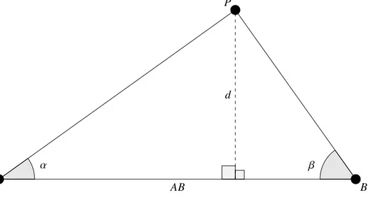
Triangulation can be used if we have two known points and know the bearing from these points to the tracked point P (See figure 7).

P

AB

d

A B

α β

Figure 7. Triangulation to find position of point P.

If the distance between point A and B is known as well as the angles α and β. The distance AB can be written as: AB= d tan α + d tan β (3.13) AB= d( 1 tan α + 1 tan β) (3.14) Trigonometric identity:

tan θ = _{cos θ}sin θ 1

tan θ = cos θ

sin θ (3.15)

Using the trigonometric identity 3.15 in 3.14 the following:

AB= d cos α sin α +

cos β sin β !

AB= d sin β cos α + sin α cos β sin α sin β

!

(3.16) The identity of sum of angles:

sin(θ + γ) = sin θ cos γ + cosθ sin γ (3.17)

Using the identity of sum of angles 3.17 in 3.16 the following expression for the distance d: AB= d sin(α + β) sin α sin β ! d = AB sin α sin β sin(α + β) ! (3.18) Using the distance d the full coordinates for the point P can be derived using the first part of

equation 3.13. Assuming that point A is positioned at the origin the coordinates for the point P can be described as ( d

4.

Tracking Techniques

Depending on the application different tracking techniques may be more or less suitable. The following chapter contains a review of the most common tracking technologies used for VR.

4.1.

Mechanical trackers

The basic type of mechanical tracker connects multiple rods and rotary encoders to the tracked object. By measuring the angles of the rods, the position of the tracked object can be calculated via forward kinematics. The rotary encoders can either be absolute or relative. Absolute encoders measure the absolute angle via potentiometers, which can be sensitive to wear and tear. Relative encoders measure angular velocity and are less sensitive to wear, but require initialization to give correct orientation angles. They also suffer from drift due to error accumulation (see section 3.1).

Mechanical trackers can suffer from a phenomena called gimbal lock. This is when two axes of the tracking system lines up, which reduces the available degrees of freedom by one, thus physically restricting movement. The physical rods used to connect the tracked object to the rotary encoders can also obstruct the view in augmented reality systems.

Benefits Mechanical trackers have good precision and high accuracy. They also have high update rate

and low lag.

Drawbacks Since the user is connected to a mechanical contraption the working volume is limited.

The user’s movement can be hampered and if used in combination with augmented reality the view can be obstructed. The tracker can also end up in gimbal lock.

4.2.

Acoustical trackers

Most acoustical trackers work by having small speakers positioned around the tracking volume. These speakers emit periodic ultrasonic sound pulses. The tracked object is fitted with microphones which register the emitted sound pulses from the speakers. By measuring the time of flight of the sound signal from emission to reception the distance from microphone to speaker can be calculated. By combining multiple measurements from different speakers a position in 3D space can be inferred via trilateration (see section 3.2). An alternative method used by Sutherland (1968) is to measuring the phase shift between the transmitted signal and the detected signal, but this method only gives relative changes.

Benefits The sensors are small and lightweight. It is possible to use multiple receivers in the same

tracking volume.

Drawbacks Update rate is limited by the speed of sound. The sensors are sensitive to acoustic noise

and occlusions. They are also sensitive to changes in wind, temperature- and humidity.

4.3.

Electromagnetic trackers

Magnetic trackers work by having a base station which emits magnetic fields, alternating between three orthogonal axes. The tracked object is fitted with sensors which can measure this generated magnetic field. This results in measurement of both position and orientation.

Users with pacemakers and other types of medical implants, which could be sensitive to electromagnetic fields, should avoid using these types of trackers.

Benefits The resulting precision and accuracy are very good. Another benefit is high update rate and

low latency. The sensors are small and lightweight. There is no visual occlusion problem.

Drawbacks The sensors are sensitive to electromagnetic noise and ferromagnetic materials. Accuracy

decreases with distance, as the magnetic field decreases with the cube of the distance to the base station (1/r3_).

4.4.

Inertial trackers

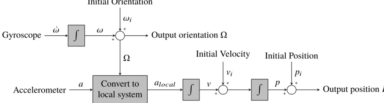
Inertial trackers works by measuring angular velocities and linear accelerations. Angular velocity can be measured using a gyroscope and then integrated to get a relative orientation change since the last measurement. Linear acceleration can be measured by an accelerometer. These have to be integrated twice to get a position (see figure 8). Inertial trackers are relative in their nature, i.e. they measure orientation and position relative an initial starting condition. Any error due to noise or bias in the gyroscopes or accelerometers will lead to drift, since errors will accumulate over time (see section 3.1). The drift in orientation can be corrected using a gravimetric inclinometer and a compass. The fact that gravity points downwards can be used as a reference signal to correct for drift in pitch and roll. A compass points north which can be used to correct for drift in yaw. To correct positional drift some other outside tracking technology is needed (see section 4.7).

Inertial sensors used to be quite large, but since the advent of microelectromechanical systems (MEMS) their size have been reduced drastically. This has also enabled mass production and substantial cost reduction (Maenaka, 2008). R + + Convert to local system R + + R Gyroscope Accelerometer Output orientation Ω + + Output position P

Initial Velocity _{Initial Position} Initial Orientation ˙ω ω Ω a alocal v p vi pi ωi

Figure 8. Calculating position P and orientation Ω from gyros and accelerometers.

Benefits Inertial trackers have good precision and high update rate. The sensors are very small and

lightweight sensors. There is no occlusion problem.

Drawbacks The only give relative positions and orientation, which leads to accumulative error over

time (drift).

4.5.

Optical trackers

Optical trackers work by projecting special patterns of light (i.e. structured light) over the desired tracking volume. The tracked object is fitted with light sensors which can detect changes in light. The position can be calculated using knowledge of the light pattern and the information from the light sensor. Some systems use a sweeping light pattern and uses the timing information from the light sensors calculate the position via triangulation (see section 3.3).

The light sensor on the tracked object may be occluded by the user in certain positions. To remedy this problem multiple light projection engines may be used to emit light from different directions. Another option is to use multiple sensors.

Benefits Optical trackers have low input delay and high accuracy. Drawbacks The sensors can be occluded in certain positions.

4.6.

Video trackers

Video trackers employ cameras and image processing to track objects. The camera can be placed on the tracked object looking at fixed objects in the environment. This type of tracking is known as inside-out tracking. Another option is to have the camera fixed and looking at the tracked object, which is known as outside-in tracking. Outside-in tracking is more susceptible to occlusions problems, but have the benefit of not having to equip the tracked object with a potentially heavy camera.

The cameras can track special markers, known as fiducial markers. These can be objects or special patterns which are easily detected by the camera and uniquely identifiable (see figure 9).

Figure 9. Example of fiducial markers used for image based trackers.

Another option is to fit the camera with IR-light sources and the tracked object with reflective targets. By filtering all light but the IR-spectrum the camera can only see the reflective targets.

A third option is to use markerless tracking which works by detecting features in the images and use those features to track the changes between images. This is a more image processing intensive method. Video trackers was previously avoided due to image processing delay, as well as both the cost and performance of digital imaging systems. But this has changed as computers have become faster and digital image systems have become both better and less expensive. Video see-through systems are natural targets for this type of tracking solution since they are already fitted with cameras.

Benefits Video trackers enable multiple tracked objects in the same tracking volume. They have good

precision and accuracy.

Drawbacks Image processing delay which may be noticeable. Can be sensitive to optical noise and

changing lighting conditions within the tracking volume. The tracked targets may be occluded in situations when using outside-in tracking.

4.7.

Hybrid trackers

Hybrid solutions is often used to employ specific strengths of certain tracking technology, while remedying the drawbacks by utilizing a complementary technology. For example combining a high rate relative tracker with low rate absolute tracker in an effort to reduce drift. Another combination can be to combine trackers which are sensitive to occlusion with trackers which are not. Combining tracker technologies requires sensor fusion techniques, such as Kalman Filtering (Welch, 2009) or other statistical sensor fusion methods.

4.8.

Full body tracking

Sometimes there is a desire to track the users hands with finger movement, such as grasping or pointing. Some application even tries to track the entire body of the user, such as visual effects in movies and games, medical applications or sports. This can be performed by attaching tracking sensors to the limbs of the person such as electromagnetic, inertial or optical sensors. Another option is to attach reflective tracking targets and using a video tracker. It is also possible to use mechanical tracking. By attaching rotary encoders to the joints of the person and forward kinematics can be used to calculate the current pose. Yet another option is to use optical fibers along limbs and joints. When the user bends a joint the light intensity in the optical fiber attenuates. Using this light attenuation the pose of the joint can be calculated. This type of technology is mostly used for finger tracking in VR-gloves.

5.

Tracking for Automotive Virtual Reality Applications

Using real vehicles on test tracks are a common way of performing vehicle testing. But driving simulators have traditionally been used if the scenarios are too dangerous, too complex or if there is need for strict respectability. But the motion feedback in a driving simulator may cause motion

sickness, which in turn make the drivers adapt their behavior (Kemeny and Panerai, 2003). As a remedy Bock et al. (2005) proposed using virtual reality inside a real vehicle in an effort to gain some of the benefits from driving simulators when performing tests using real vehicles. This is performed by driving a real vehicle on a test track, but letting the driver interact with a virtual environment and virtual targets.

One benefit of using virtual targets is the possibility to handle scenarios with complex interactions between actors. Another benefit is that a collision with a virtual target would lack physical consequence for either vehicle or driver. The concept of driving in real vehicles using virtual reality or augmented reality have been investigated further to validate driver behavior in several different studies (Bock et al., 2007; Karl et al., 2013).

5.1.

Tracking the vehicle

Most traditional tracking systems are designed to room scale tracking volumes or smaller. To be able track objects in larger spaces (i.e. larger than room scale) other technologies must be utilized.

Satellite navigation There are currently two operational global satellite based navigation systems

(GNSS); GPS (USA) and GLoNaSS (Russia). Two more are in development; Galileo (EU) and BeiDou (China). These use systems trilateration (See section 3.2) to calculate a ground position. The accuracy of these types of system are approximately 101_{meters. The accuracy of these types}

of systems can be further improved by using a Differential-GPS (DGPS), i.e. using a ground base station positioned at a well known position. The accuracy using DGPS are approximately 10−1

meters. Another way of improving precision is to use Real-time Kinematic Positioning (RTK), i.e measuring the carrier phase of the GNSS signal. This requires two receivers, but can enhance the precision down towards 10−2_meters.

The drawbacks with GNSS is that it requires a free sky, i.e. it cannot be used indoors and can have problems in environments which have high buildings or large trees with dense foliage.

Odometry When tracking vehicles using either wheels or tracks, the odometry data can be used to

perform dead reckoning (See section 3.1). Odometry data can be captured by measuring wheel revolutions. The quality of tracking depends on the precision of this data and can be easily disturbed if the wheels slips or skids. Instead of measuring wheel revolutions one option is to use non-contact measurements of speed-over-ground velocities. This can be achieved using optical measurement systems or Laser Doppler velocimetry, which uses the Doppler shift in a laser beam to measure the velocity of the ground surface relative to the vehicle.

Image based Using image based simultaneous localization and mapping (SLAM) techniques relative

positions and orientations can be calculated with high accuracy (Dissanayake et al., 2011). But these techniques can have high latency due to image processing delay.

In the first paper by Bock et al. (2005) a optical odometry system was used to track the relative movements of the vehicle, but in subsequent studies (Bock et al., 2007; Karl et al., 2013) DGPS was used.

5.2.

Tracking inside the vehicle

Tracking the user inside a vehicle may have consequences for the measured accuracy and precision. Special considerations have to be made when selecting the tracking technology:

Mechanical Using mechanical trackers inside a vehicle is possible. The driver movement is already

constrained by the car seat and could probably be tracked using a custom mechanical linkage system.

Acoustical Acoustical trackers are unsuitable due to the noisy environment of inside a vehicle.

Electromagnetic Vehicles contains quite lot of ferromagnetic materials and are filled with electronics,

which causes distortions in the magnetic field.

Inertial Inertial trackers can be used but the inertial information from the vehicle must be subtracted

from the inertial information of the tracker inside the vehicle. Foxlin (2000) successfully used inertial trackers inside a driving simulator with a moving base, results that possibly could be transferable real vehicle conditions.

Optical Vehicles are driven outside which results in quite a lot of sunlight entering the cabin. Any

optical tracking system used must be robust enough to be able to track targets in these conditions.

Video These types of trackers have the same problems as optical trackers with incoming sunlight in the

cabin. Tracking cameras using automatic aperture control can also be disturbed by fast changing light conditions.

In the first papers by Bock et al. (2005, 2007) a optical tracker based on laser light was used to track the driver head position and orientation. While the study by Karl et al. (2013) used a video tracker

6.

Conclusions

Using virtual reality requires some form of tracking to present the correct view to the user.

This publication has presented the most common contemporary technologies for tracking and their corresponding algorithms. It is important to select the appropriate tracking technology for the desired application.

Using virtual reality in an automotive context put additional demands on the selected tracker. This is due to the environment inside the vehicle; the vehicle is moving, the lighting conditions change as the car moves, the acoustical noise levels are high, and most vehicles are filled with lots of magnetic materials as well as electronics. This make the vehicle a very hard environment to use traditional tracking technologies without advanced correction.

If the user should interact with objects outside the vehicle then the vehicle needs to be tracked with high precision as well. Satellite navigation can be used to give an absolute position. Odometry can be used to measure the relative motion with high precision. A recent option is to use image based SLAM solutions to track the vehicle.

References

B. Danette Allen, Gary Bishop, and Gregory F. Welch. Tracking: Beyond 15 Minutes of Thought. In

SIGGRAPH Course Pack, 2001.

Ronald T. Azuma and Gary Bishop. A frequency-domain analysis of head-motion prediction. In Proceedings of the 22nd annual conference on Computer graphics and interactive techniques

-SIGGRAPH ’95, pages 401–408, New York, NY, USA, 1995. ACM Press. doi: 10.1145/218380.

218496.

Devesh Kumar Bhatnagar. Position trackers for Head Mounted Display systems : A survey. Technical report, University of North Carolina, Chapel Hill, North Carolina, USA, 1993.

Gary Bishop and Henry Fuchs. Research directions in virtual environments: report of an NSF Invitational Workshop, March 23-24, 1992, University of North Carolina at Chapel Hill. ACM

SIGGRAPH Computer Graphics, 26(3):153–177, aug 1992. doi: 10.1145/142413.142416.

Thomas Bock, Karl-Heinz Siedersberger, and Markus Maurer. Vehicle in the Loop - Augmented Reality Application for Collision Mitigation Systems. In Fourth IEEE and ACM International

Symposium on Mixed and Augmented Reality (ISMAR’05), Vienna, Austria, 2005. IEEE Computer

Society. doi: 10.1109/ISMAR.2005.62.

Thomas Bock, Markus Maurer, and Georg Färber. Validation of the Vehicle in the Loop (VIL) - A milestone for the simulation of driver assistance systems. In Proceedings of the 2007 IEEE Intelligent

Vehicles Symposium, pages 219–224, Istanbul, Turkey, 2007. IEEE. doi: 10.1109/IVS.2007.4290183.

Carolina Cruz-Neira, Daniel J. Sandin, and Thomas A. DeFanti. Surround-screen projection-based virtual reality. In Proceedings of the 20th annual conference on Computer graphics and interactive

techniques - SIGGRAPH ’93, pages 135–142, New York, New York, USA, 1993. ACM Press. ISBN

0897916018. doi: 10.1145/166117.166134.

Gamini Dissanayake, Shoudong Huang, Zhan Wang, and Ravindra Ranasinghe. A review of recent developments in Simultaneous Localization and Mapping. In 2011 6th International Conference on

Industrial and Information Systems, pages 477–482. IEEE, aug 2011. doi: 10.1109/ICIINFS.2011.

6038117.

David Drascic and Paul Milgram. Perceptual issues in augmented reality. SPIE Volume 2653:

Stereoscopic Displays and Virtual Reality Systems III, 2653:123–134, 1996.

Frank J Ferrin. Survey of helmet tracking technologies. In Large Screen Projection, Avionic, and

Helmet-Mounted Displays, volym 1456, pages 86–94, 1991. doi: 10.1117/12.45422.

Eric Foxlin. Head tracking relative to a moving vehicle or simulator platform using differential inertial sensors. Proceedings of SPIE: Helmet and Head-Mounted Displays V, 4021:133–144, 2000. doi: 10. 1117/12.389141.

Eric Foxlin. Motion tracking requirements and technologies. In Handbook of virtual environment

technology, chapter 8, pages 163–210. CRC Press, Mahwah, NJ, USA, 2002. ISBN 080583270X.

Jason J Jerald, Tabitha Peck, Frank Steinicke, and Mary C. Whitton. Sensitivity to scene motion for phases of head yaws. In Proceedings of the 5th symposium on Applied perception in graphics and

visualization - APGV ’08, pages 155–162, New York, NY, USA, 2008. ACM Press. doi: 10.1145/

1394281.1394310.

Ines Karl, Guy Berg, Fabian Ruger, and Berthold Färber. Driving Behavior and Simulator Sickness While Driving the Vehicle in the Loop: Validation of Longitudinal Driving Behavior. IEEE Intelligent

Transportation Systems Magazine, 5(1):42–57, 2013. doi: 10.1109/MITS.2012.2217995.

Andras Kemeny and Francesco Panerai. Evaluating perception in driving simulation experiments.

Kazusuke Maenaka. MEMS inertial sensors and their applications. In 2008 5th International

Conference on Networked Sensing Systems, number c, pages 71–73. IEEE, jun 2008. ISBN

978-4-907764-31-9. doi: 10.1109/INSS.2008.4610859.

Paul Milgram, Haruo Takemura, Akira Utsumi, and Fumio Kishino. Augmented reality: A class of displays on the reality-virtuality continuum. Telemanipulator and Telepresence Technolgies, 2351:282– 292, 1994.

Jannick P. Rolland, Larry D. Davis, and Yohan Baillot. A survey of tracking technology for virtual environments. In Fundamentals of Wearable Computers and Augmented Reality, chapter 3, pages 67– 112. CRC Press, Hillsdale, NJ, USA, 2001. ISBN 0805829024.

Ivan E. Sutherland. A head-mounted three dimensional display. In Proceedings of the December 9-11,

1968, Fall Joint Computer Conference, Part I, AFIPS ’68 (Fall, part I), pages 757–764, New York, NY,

USA, 1968. ACM. doi: 10.1145/1476589.1476686.

Colin Ware, Kevin Arthur, and Kellogg S Booth. Fish tank virtual reality. In Proceedings of the

SIGCHI conference on Human factors in computing systems - CHI ’93, pages 37–42, New York, New

York, USA, 1993. ACM Press. ISBN 0897915755. doi: 10.1145/169059.169066.

Gregory F. Welch. HISTORY: The Use of the Kalman Filter for Human Motion Tracking in Virtual Reality. Presence: Teleoperators and Virtual Environments, 18(1):72–91, feb 2009. doi: 10.1162/pres. 18.1.72.

www.vti.se

VTI, Statens väg- och transportforskningsinstitut, är ett oberoende och internationellt framstående forskningsinstitut inom transportsektorn. Huvuduppgiften är att bedriva forskning och utveckling kring

infrastruktur, trafi k och transporter. Kvalitetssystemet och

miljöledningssystemet är ISO-certifi erat enligt ISO 9001 respektive 14001. Vissa provningsmetoder är dessutom ackrediterade av Swedac. VTI har omkring 200 medarbetare och fi nns i Linköping (huvudkontor), Stockholm, Göteborg, Borlänge och Lund.

The Swedish National Road and Transport Research Institute (VTI), is an independent and internationally prominent research institute in the transport sector. Its principal task is to conduct research and development related to infrastructure, traffi c and transport. The institute holds the quality management systems certifi cate ISO 9001 and the environmental management systems certifi cate ISO 14001. Some of its test methods are also certifi ed by Swedac. VTI has about 200 employees and is located in Linköping (head offi ce), Stockholm, Gothenburg, Borlänge and Lund.

HEAD OFFICE LINKÖPING SE-581 95 LINKÖPING PHONE +46 (0)13-20 40 00 STOCKHOLM Box 55685 SE-102 15 STOCKHOLM PHONE +46 (0)8-555 770 20 GOTHENBURG Box 8072 SE-402 78 GOTHENBURG PHONE +46 (0)31-750 26 00 BORLÄNGE Box 920 SE-781 29 BORLÄNGE PHONE +46 (0)243-44 68 60 LUND Medicon Village AB SE-223 81 LUND PHONE +46 (0)46-540 75 00