BATTERY SENSORY DATA COMPRESSION FOR ULTRANARROW BANDWIDTH IOT PROTOCOLS

(1)

V¨aster˚as, Sweden

Thesis for the Degree of Master of Science in Computer Sciences with Specialization in Embedded Systems 15.0 credits

BATTERY SENSORY DATA

COMPRESSION FOR ULTRA

NARROW BANDWIDTH IOT

PROTOCOLS

Ahmed Karic akc17002@student.mdh.se

Ivan Loncar ilr17002@student.mdh.se

Examiner: Moris Behnam

M¨alardalen University, V¨aster˚as, Sweden

Supervisor: Tran Hung

Mälardalen University, Väster˚as, Sweden Company supervisor: Ralf Strömberg,

ADDIVA AB, V¨aster˚as, Sweden

(2)

Abstract

Internet of Things (IoT) communication technology is an essential parameter in modern embedded systems. Demand for data throughput drastically increases, as well as the request for transmission over considerable distance. Considering cost-efficiency in the form of power consumption is unavoidable, it usually requires nu-merous optimization and trade-offs. This research tends to offer a solution based on data compression techniques. In this way, problems caused by data through-put are mostly eliminated, still varying with the field of application. Regardless of having both lossy and lossless techniques, the focus is on lossy algorithms due to immensely larger compression ratio (CR) factor, which is not the only but usually the most crucial factor. There are also numerous other quality metrics described. In the experiment part, LoRa long-range wireless communication protocol is used, with an accent on battery sensory data transmission. Temperature and current are the signals of interest. The research offers detailed information of the impact on compression parameters by four target algorithms: fractal resampling (FR), critical aperture (CA), fast Fourier transform (FFT) and discrete cosine transform (DCT).

(3)

List of plots

6.1 Data acquisition block diagram . . . 17

7.1 Data transmission block diagram . . . 20

8.1 The first midpoint, arithmetic mean of the first and the last point in the sequence: x(4) . . . 30

8.2 Sequence divided into two sub-sequences, arithmetic means at x(2) and x(6) . . . 30

8.3 Arithmetic means at x(1), x(3), x(5) and x(7) . . . 30

8.4 Signal plot of the original and compressed data . . . 30

8.5 Initial slope with x(0) and x(1), further points x(2), x(3) and x(4) -x(3) stored . . . 31

8.6 Slope generated with x(3) and x(4). Unsuccessful check at point x(5) - x(4) stored . . . 31

8.7 Referent slope with with x(4) and x(5) - x(6) stored . . . 31

8.8 Original and compressed signal on the same plot . . . 31

8.9 Data split process from the initial data set to the pairs . . . 32

8.10 Backward calculation of the coefficients on sub-levels. Cooley-Tukey FFT with time decimation for N=8 . . . 32

9.1 Overall representation of the system setup . . . 35

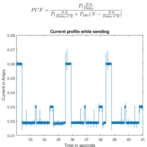
10.1 Current consumption profile of Sodaq board while sending data with 400 ms air time . . . 40

10.2 Current consumption profile of Sodaq board while idle . . . 41

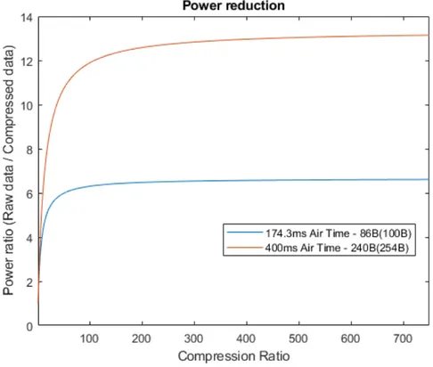
10.3 Power reduction ratio for different packet size and air times for Sodaq board . . . 41

10.4 CR - PRD dependence for current signal . . . 42

10.5 CR - PRD dependence for voltage signal . . . 42

10.6 CR - PRD dependence for temperature signal . . . 43

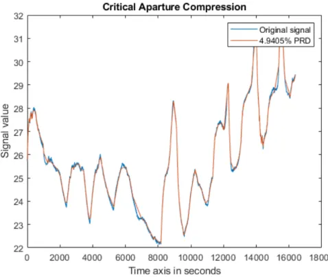
10.7 Reconstruction of current data compressed by CA, with amperes(A) on Y-axis and PRD close to 5% . . . 44

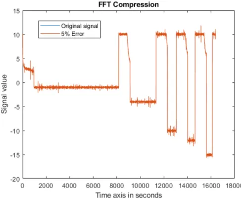
10.8 Reconstruction of current data compressed by FFT, with amperes(A) on y-axis and PRD close to 5% . . . 44

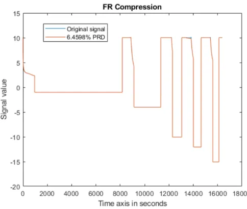
10.9 Reconstruction of current data compressed by, with amperes(A) on y-axis and PRD close to 5% . . . 45

10.10Reconstruction of current data compressed by DCT, with amperes(A) on y-axis and PRD close to 5% . . . 45

10.11Reconstruction of voltage data compressed by CA, with volts on y-axis and PRD close to 5% . . . 46

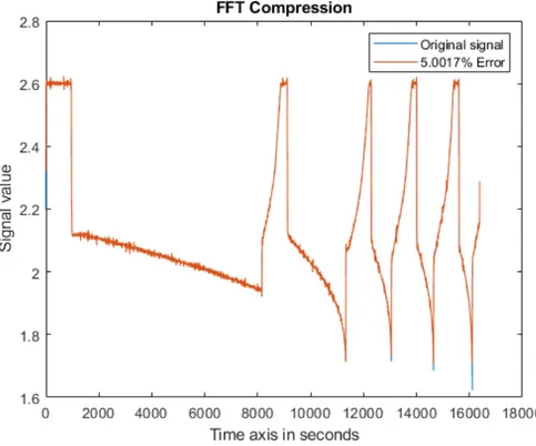
10.12Reconstruction of voltage data compressed by FFT, with volts on y-axis and PRD close to 5% . . . 46

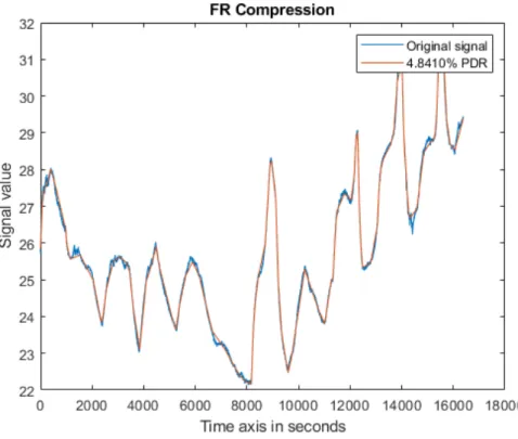
10.13Reconstruction of voltage data compressed by FR, with volts on y-axis and PRD close to 5% . . . 47

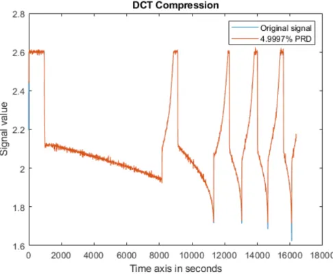
10.14Reconstruction of voltage data compressed by DCT, with volts on y-axis and PRD close to 5% . . . 47

10.15Reconstruction of temperature data compressed by CA, with celsius on y-axis and PRD close to 5% . . . 48

(4)

10.16Reconstruction of temperature data compressed by FFT, with celsius

on y-axis and PRD close to 5% . . . 49

10.17Reconstruction of temperature data compressed by, with celsius on y-axis and PRD close to 5% . . . 49

10.18Reconstruction of temperature data compressed by DCT, with celsius on y-axis and PRD as close to 5% . . . 50

A.1 CA compression of voltage signal with 1% absolute error . . . 55

A.2 CA compression of voltage signal with 5% absolute error . . . 55

A.3 CA compression of current signal with 1% absolute error . . . 55

A.4 CA compression of current signal with 5% absolute error . . . 55

A.5 CA compression of temperature signal with 1% absolute error . . . . 55

A.6 CA compression of temperature signal with 5% absolute error . . . . 55

A.7 DCT compression of voltage signal with 1% absolute error (in ampli-tude spectra) . . . 56

A.8 DCT compression of temperature signal with 1% absolute error (in amplitude spectra) . . . 56

A.9 DCT compression of current signal with 1% absolute error (in ampli-tude spectra) . . . 56

A.10 DCT compression of current signal with 5% absolute error (in ampli-tude spectra) . . . 56

A.11 FFT compression of voltage signal with 1% absolute error (in ampli-tude spectra) . . . 56

A.12 FFT compression of temperature signal with 1% absolute error (in amplitude spectra) . . . 56

A.13 FFT compression of current signal with 1% absolute error(in ampli-tude spectra) . . . 57

A.14 FFT compression of current signal with 5% absolute error(in ampli-tude spectra) . . . 57

A.15 FR compression of voltage signal with 1% absolute error . . . 57

A.16 FR compression of voltage signal with 5% absolute error . . . 57

A.17 FR compression of current signal with 1% absolute error . . . 57

A.18 FR compression of current signal with 5% absolute error . . . 57

A.19 FR compression of temperature signal with 1% absolute error . . . . 58

(5)

Tables

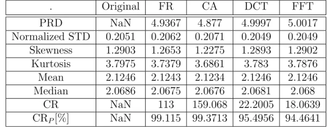
1 Table comparing parameters of original current signal to reconstructed signal with different compression algorithms (Sample size = 16384) . 43 2 Table comparing parameters of original voltage signal to reconstructed

signal with different compression algorithms (Sample size = 16384) . 43 3 Table compares parameters of original temperature signal to

recon-structed signal for different compression algorithms (Sample size = 16384) . . . 48 4 Table compares parameters of original voltage signal to reconstructed

signal for different compression algorithms with absolute error bound of 1% (Sample size = 16384) . . . 58 5 Table compares parameters of original voltage signal to reconstructed

signal for different compression algorithms with absolute error bound of 5% (Sample size = 16384) . . . 58 6 Table compares parameters of original current signal to reconstructed

signal for different compression algorithms with absolute error bound of 1% (Sample size = 16384) . . . 59 7 Table compares parameters of original current signal to reconstructed

signal for different compression algorithms with absolute error bound of 5% (Sample size = 16384) . . . 59 8 Table compares parameters of original temperature signal to

recon-structed signal for different compression algorithms with absolute er-ror bound of 1% (Sample size = 16384)) . . . 59 9 Table compares parameters of original temperature signal to

recon-structed signal for different compression algorithms with absolute er-ror bound of 5% (Sample size = 16384) . . . 60

(6)

Acknowledgements

We take this opportunity to express our gratitude to the company ADDIVA ELEK-TRONIK AB for offering an opportunity to perform a research in a wonderful envi-ronment. Addiva supplemented us with all necessary equipment and offered a support by great staff. We hereby thank to Peter, Ralph, Nills, Oly, Rasmus and Madalen. We also owe a huge gratitude to our supervisor Tran Hung for unselfish dedication to our work and support in the report.

(7)

Acronyms

IoT Internet of Things CR Compression Ratio FR Fractal Resampling CA Critical Aperture

FFT Fast Fourier Transformation DCT Discrete Cosine Transformation RTOS Real Time Operating System IDE Integrated Development Environment RT Real Time

CPU Central Processing Unit MAC Media Access Protocol OSI Open System Interconnection ISM Industrial, Scientific and Medical CH Chebyshev transform

WPD Wavelet Packet Decomposition ECG Electrocardiogram

PPG Photoplethysmogram

DWT Discrete Wavelet Transform

FWHT Fast Walsh-Hadamard Transform LDE Lossy Delta Encoding

ML Machine Learning

ADC Analog to Digital Conversion MWC Modulated Wideband Converter ASEC Analysis by Synthesis Coding RMS Root Mean Square

PRD Percentage RMS Difference WDD Weighted Diagnostic Distortion

(8)

DFT Discrete Fourier Transform SVD Singular Value Decomposition PAA Piecewise Aggregate Approximation

APCA Adaptive Piecewise Constant Approximation PLA Piecewise-Linear Approximation

VLSI Very Large Scale Integration DSP Digital Signal Processing PCA Principal Component Analysis MCU Microcontroller Unit

SoC State of Charge IC Integrated Circuits

NTC Negative Temperature Coefficient PTC Positive Temperature Coefficient RLE Run Length Encoding

BS Backward Slope BC Box Car

CF Curve Fitting

NASA National Aeronautics and Space Administration STD Normalized Standard Deviation

TTN The Things Network PCF Power Consumption Factor

(9)

1 Introduction

In the world of the IoT technology, demand for low power - long range sensory data transmission is rapidly growing. ”In IoT, numerous and diverse types of sensors generate a plethora of data that needs to be stored and processed with minimum loss of information ”[1]. Networked embedded devices are generating a vast amount of data that need to be sent to the cloud, and then processed and stored. Applica-tion areas are mainly related to transportaApplica-tion, medical, health-care, military and agriculture. Some of the applications, like car battery monitoring and smart farms, require the data to be sent over a long distance with some power restriction. This thesis propose an analysis of a battery management system concerning all essential parameters, which can be processed and controlled to prolong battery life.

Data is created in the embedded networked devices, or more commonly known as IoT devices usually, need to be analyzed by a remote server computer. How-ever, communication problems arise on different stages, mostly on end-point-devices, where all the information is gathered. The data is supposed to be frequently sent via long range-low power wireless network, low bandwidth limits that. These types of network can fail in sending the data, or in some cases succeed, but with lower transmission rates. Such data would be stored in the memory of the end-device un-til it is getting resent. Considering the worst cases, the memory may get saturated in some instance. Problem with the lack of memory could be solved using data compression technique. Regardless of the presence and accessibility of the future communication protocols, the data compression process will be an inevitable and unavoidable factor.

Depending on the use-case of networked embedded devices different IoT protocols can be utilized. Low power-long range protocols are needed for the energy efficient devices that depend on batteries and are transmitting data over long distances, which may be several kilometers. Pure representatives of wireless IoT protocols, which are long range and low power are Ingenu, LoRa, SigFox, listed in the article [2], as the examples of company developed, Symphony based on LoRa physical layer, and Weightless as examples of open source protocols. Ingenu protocol is not universal in a sense it is only situated in the North American territory and proposed for local needs. Thus it will not be evaluated in this research. Open source variants of wireless protocols, mentioned above, also will not be considered due to poor support from the community and not well developed. To the best of our knowledge, SigFox and LoRa are feasible for protocols that will be analyzed and compared for different purposes in implementation and the research.

2 Problem Formulation

The core problematic revolves around the comparison and analysis of specific data compression algorithms for optimizing of battery system features. Essential feature constraints are put on power consumption, real time performance, memory and processor demand.

At the very beginning, it is necessary to analyze sampling rate of multiple sen-sory data, to evaluate compression algorithm complexity, communication properties,

(12)

as well as the selection of real time operating system (RTOS), to determine which microcontroller and central processing unit (CPU) is best for the specific require-ments.

Many different compression algorithms will be tested and compared. Desired comparison properties of the algorithms are mainly related to the algorithm execu-tion complexity, losses, level of compression and need for memory extension. Hence, the following research questions are in the primary focus of the thesis:

RQ1: What is the CR factor of different compression algorithms applied on battery data?

RQ2: What is the effect of specific compression algorithms on memory capacity and power consumption?

3 Method

To achieve an effective research on the topic, case study is employed in the first half of the research, where multiple papers will be reviewed. Numerous compression techniques, applied in different areas, are analyzed in order to acquire the most suitable ones for the target application.

After the analysis, appropriate algorithms are selected and tested in an exper-iment setup. The experexper-iment is obtained to give answers to RQ2. It was mainly based on observing current behaviour in the transmitting node. Thus the research is represented as a combination of case study method with the experiment.

Research process is obtained through the following steps: 1 - Analysis of selected data compression algorithm.

2 - Select the most suitable algorithms for the field of application. It is not manda-tory to apply only existing compression algorithm. The research will be supple-mented by some of the well-known numerical methods or different approaches in data reduction techniques.

3 - Analysis of all essential parameters for development environment: a processing unit, development board and RTOS . The parameters that will be considered are the memory, power consumption, clock frequency, the case of implementation and integrated development environment (IDE).

4 - System setup: setting Lora network, hardware and software setup, testing the system. To attain valid results, signal measurements on current, voltage and temperature data will be measured and stored in a file on a personal computer. The data is used for testing, to have reproducible and consistent results.

5 - Implementation and testing of selected compression algorithms. Tests compare algorithms power consumption, real time (RT)1 _{capabilities and compression}

ratio (CR), with respect to error margin for lossy compression.

1_{Real time property of an algorithm represents its capability to obtain compression during}

(13)

6 - Analyzing and comparing the results based on different metrics to determine the effectiveness of the data reduction techniques and providing a significant suggestion.

4 Background

In the field of transportation, battery technology is known as future energy system solutions. There are many vehicle types powered by battery technology. To prolong battery lifetime, sustainable maintenance is required, and accurate monitoring of en-ergy measurements can achieve this. Importantly, we need to measure and control battery electrical energy consumption, regarding current, voltage, and temperature, as important battery-life parameters. To have access and to be able to manipulate with the battery parameters, it is necessary to make them available on the servers via the appropriate wireless communication protocol. The communication should contain an end-device, also called node, a low power device that performs data ac-quisition. The data are further sent to the antenna, called gateway, that receives information from the node, and can feedback the data to the node. It is necessary to keep in mind that the end-device must belong to some of the three possible end-node classes: A, B or C. Detailed information about the classes are available on [3]. An end-device, belonging to any of the classes, must support bi-directional communica-tion with the gateway [3]. In the implementacommunica-tion part (see chapter System setup), the role of the node-device is delivered to AVR32’s EVK1100 board, which for the experimental part of the research will not include any sensor, due to confidentiality reasons.

Particular wireless protocols provide the low power transmission of data over long distance (up to 15 kilometers), and their well-known representatives are LoRa and SigFox. The protocols fit the description of possible applications, but on the other hand, have huge limitations on data throughput.

LoRaWAN is a low power-long range media access protocol (MAC), which belong to the second (data-link) and the third (network) layer of Open Systems Intercon-nection (OSI) reference model [4]. Its operating frequency varies with location. It operates in 863-870 MHz in Europe, US 902-928 MHz, China 779-787 and 470-510 MHz. Data bandwidth of the protocol rises to maximal 500 kHz, still depending on the region of the application. Its modulation is based on Chirp2technology[5], which ensures the communication to work properly and immune to noise and Doppler ef-fect even at low power consumption. In the US, LoRa has dedicated uplink and downlink channels. Eight uplink channels are operating on 125 kHz, one 500 kHz uplink channel and one 500 kHz down-link channel[3].

Its first concurrent, SigFox, has also established wide application area, being part of Industrial, Scientific and Medical (ISM) radio band. It operates on 868 MHz in Europe and 902 MHz in the US. The network has a star-topology and ability to cover a huge area. ”Sigfox operate in the 200 kHz of the publicly available band to exchange radio messages over the air. Each message is 100 Hz wide and transferred

2_{CHIRP ( Compressed High-Intensity Radiated Pulse) is a technology that has been used in}

(14)

at 100 or 600 bits per second a data rate, depending on the region. Hence, long distances can be achieved while being very robust against the noise”[6].

To preserve the quality of the information subject to constraints of transmission rates, it is necessary to reduce the size of data by applying compression algorithms. Compression can be either lossless or lossy. The lossless principle is the one where no data is lost, but all the redundancies are removed. In the case of lossy algorithms, data fidelity is being lost within predefined error margins. Many use cases allow data to be lost, so lossy compression is usually implemented when higher compression ratios are required.

To achieve effective research on the topic, mixed methods of case study and experiment will be combined. The case study provides an investigation and quan-titative comparison of state of the art compression algorithms and a general way a data reduction can be achieved. On the other hand, when testing and comparing specific algorithms, experiment setup yields a quantitative approach for answering the research questions. As previously stated in the research questions, RQ1 and RQ2 can only be answered by executing an experiment and comparing obtained results.

Regarding the final expectations, a goal is to find optimal compression algorithm for networked embedded devices or IoT solutions that require data reduction. Opti-mum solution in this investigation refers to keeping the real time capabilities of the system within small boundaries of error tolerance.

5 Related Work

There exists a wide variety of compression algorithms with different classifications ranging from lossless and lossy ones, from the time domain to transfer domain ones, and from general ones to data specific ones like algorithms for the image, video, and text. This thesis aims towards lossy algorithms with a limited amount of loss of data fidelity. Each type of sensor has, a unique signal characteristic, and they are time-varying one-dimensional signals. A paper published by Tulika Bose et.al. [1] shows a study that compares four compression algorithms on a set of six types of signals. The target algorithms are CA and FR from time domain and Chebyshev transform (CH) and Wavelet Packet Decomposition (WPD) from transform domain. Data types processed for algorithm testing are Electrocardiogram (ECG), Photoplethysmogram (PPG), bearing data as quasi-periodical signals, accelerometers and different signals form solar irradiation measurement. The authors have concluded that there is a correlation between specific types of signals and compression ratio and error margins as metrics for the number of certain compression algorithms.

The first research question is mainly related to CR factor, which highly varies depending on compression type and field of application. According to Mamaghanian et. al. [7] and the research done on compression of ECG signals, the CR (measured in percentage) ranges between 90% and 51 %, depending on the quality of the reconstruction. The research was performed on Discrete Wavelet Transform (DWT). More on CR in health application has been presented in [8] where CR factor varies between 17.6 and 44.5 and with precision up to 2.0 %. Traditionally lossy metrics perform CR between 3 and 15, whereas lossless ones range between 1 and 3 times [9].

(15)

In the research [9], hybrid model encountering both lossy and lossless compression, applied on ECG system, result in CR of 2.1 and 7.8 for lossless and lossy compression respectively. Hence, the aim is to investigate CR factors in CA applications on battery management system and a huge challenge to accomplish more than 90% of CR.

IoT devices generate huge amounts of data, that should be handled appropri-ately. According to Moon et al. it is a big challenge to find an optimal balance between a CR factor and information loss[10]. In the proposed work [10] a fea-sibility analysis of lossy compression is performed on agricultural sensor data by comparing the original and reconstructed signals. Sensors in weather stations are used as the main data resources. Among various existing algorithms the focus is put on main representatives of frequency domain compression algorithms, DCT, Fast Walsh-Hadamard Transform (FWHT), DWT and Lossy Delta Encoding (LDE). Re-sults show that DCT and FWHT have higher compression ratio than other ones. Observing the results for higher compression factors, error rates exhibit a significant increase. On the other side, LDE, compared to DCT, LDE, and DWT, allows for smaller compression factors, maintaining the error within a smaller range.

One of the most important factors in efficient operating of IoT embedded solu-tions is power consumption. The power efficiency factor can be increased in lots of communication elements, mostly related to hardware and system setup, but the core problematics revolve around the amount and speed of the data transfer. According to Stojkoska et al. [11] power consumption in preprocessing is much lower than power consumption during the transmission process. The focus of the research was put on the development of a new principle for delta compression, that results in good lossless data compression. Implementation of such an algorithm with a high level of execution complexity, demand more memory, capacity and processor power. The coding scheme proposed by Stojkovska and Nikolovski achieved up to 85% energy saving, resulting in higher compression ratio and lower memory capacity than the conventional delta coding.

As already discussed in the previous section, nodes mainly consist of sensor and controller with quite low computational power. The end-device is supplied by an external battery that is not easy to replace, in some cases even tough to access.To prolong the lifetime of the battery and the supplied node, it is necessary to reduce the data traffic, since the radio communication elements exhibit very high power consumption. In [12], efficient data compression algorithm suitable for commercial wireless sensor networks has been proposed by exploiting the principles of entropy compression.

A novel hybrid data compression scheme that reduces power consumption has been introduced by [13]. This scheme reduces power consumption in the wireless sensor by focusing on ECG application and compresses data with lossy and lossless techniques. Lossy compression with CR averaging around 7.8 saves power in wire-less transmission by 18% with Bluetooth transceiver, whereas losswire-less algorithms based on entropy coding compress residual error stored in local memory and saves 53% for raw data transmission. The residual error is extracted from raw data and reconstructed lossy data and coded with Huffman coding. They have shown that this approach can be attractive to bio-medical applications since it allows

(16)

prelim-inary signal analysis on a lossy signal, where there is no need for precise readings when the heart rhythm is stable. If abnormal heart rhythm is detected, residual data is retrieved wirelessly. This hybrid transmission method reduces energy con-sumption in all IoT applications that do not require precise data for preliminary analysis. Further improvements in power reduction can be made by using dedicated hardware and low energy wireless protocols. Also, it is possible to achieve indirect improvements by using state of the art compression algorithms, which show better performance than Fan compressor chosen in [13].

If there is no need for absolute precision, especially in applications that generate a lot of data that needs to be sent to the server via IoT networking, lossless com-pression exhibits negligible impact and show no difference, as stated by Aekyeung Moon et.al. in [14]. Their paper explores the impact of lossy compression on smart farm analytic which is highly important when making local weather predictions us-ing machine learnus-ing (ML) techniques. The importance lies in the fact that if error bounds in lossy compression algorithms discard too much useful data from the orig-inal sequence, classifying ML algorithms will not be able to give right predictions, rendering the concept of smart farming obsolete. They have shown that by achiev-ing CR of more than 99.9% with frequency domain lossy algorithms, like DCT and FWHT, ML algorithms respond with better prediction, compared to the prediction for raw data. Error bounds for lossy algorithms remove high frequency data points. Hence, removing most of the outliers makes classifiers better for predictions, and at the same time achieves high compression rates with allowed data quality loss.

Moshe Mishali and Yonina C. Eldar have introduced a way for compression al-gorithm of analog signals in the stage of analog to digital conversion (ADC) using so-called Xampling [15], where the usual scheme states that sampling rate of an ADC should be higher than the maximum occurring frequency in the signal we want to sample 3_{. Xampling is a method that reduces the amount of data in the}

sampling stage by sampling the analog signal with sub-Nyquist frequency without losing the information. One approach is a combination of sampling theory with com-pressed sensing. Comcom-pressed sensing exploits the fact that vectors in undetermined linear systems are spars (mostly zeros) and combination with random demodulation extends the idea by recovering discreet harmonics. This method although being ef-ficient is, on the other hand, challenging to implement and has high computational complexity. Xampling achieves sub-Nyquist sampling with a modulated wideband converter (MWC) which is more practical in terms of implementation and compu-tational complexity.

Yaniv Zigel et.al. have published a paper [16] that proposes a compression algo-rithm for ECG signals. A newly proposed algoalgo-rithm, analysis by synthesis coding (ASEC), exploits the predictability of measured ECG signals. ASEC adopts long and short-term predictors for compression of ECG signals with so-called beat code-book that records typical heartbeat signals. As a lossy compression algorithm that achieves CR of 30, it operates on metric for measuring distortion in the recon-structed signal with either Percentage Root Mean Square (RMS) Difference (PRD) or Weighted Diagnostic Distortion (WDD).

We mentioned some of the data reduction techniques that reduce dimensionality

(17)

such as discrete Fourier transform (DFT), DWT. There exist other techniques men-tioned and compared in research done by Kaushik Chakrabarti et.al. in [17] such as Singular Value Decomposition (SVD), Piecewise Aggregate Approximation (PAA) and their newly developed method Adaptive Piecewise Constant Approximation (APCA) that is tailored for faster and better indexing and calculation. Calculation and dimensionality reduction is made at the expense of precision, based on metrics for distance calculations in different forms of norm calculation (usually Euclidean distance norm). This novel method APCA outperforms aforementioned sophisti-cated dimensionality reduction methods by two orders of magnitude and supports arbitrary norms while being able to be indexed in a multidimensional structure. This method is also applicable to other data sequences rather than just time-series data.

In some applications of signal recording lossy compression is a desirable way of manipulating by data as mentioned in [18] Konstantinos et al. write about a piecewise-linear approximation (PLA) technique for lossy compression that can com-press signals in a given tolerance range with high comcom-pression ratio. PLA has linear computational complexity O(N ) and advantages over other techniques in frequency or time domain, not only speed-wise in the compression stage, but in reconstruc-tion as well. It is reconstructed only by linear interpolareconstruc-tion, and at the same time filters the data. As mentioned in work, the algorithm uses only a few mathemati-cal operations and comparisons which makes it easily implementable in Very Large Scale Integration (VLSI) for a single chip integration. Furthermore, improvement of compression ratio has been proposed by introducing lossless Huffman coding scheme after the lossy one.

Time series data generated by wireless sensors poses a challenge when it comes to power and memory reduction as well as keeping the RT performance of the system. This problem has been tackled by many including researchers Iosif Lazaridis and Sharad Mehrotra in their work [19]. Their task was to capture sensory data with aforementioned system performance demands with the guarantee of and result being in the range of allowed error bound based on Euclidean distance norm. To be able to reduce the amount of data being generated, not to send the raw samples that use communication bandwidth and keep RT performance, data compression has been utilized, as well as prediction scheme.

Numerous power reduction methods have been invented as a result of data reduc-tion. William R. Dieter et.al have worked on a method that changes the sampling rate of ADC by Nyquist rate [20]. Nyquist rate requires at least two times of the maximum existing frequency to produce good results. In a time-varying analog sig-nal that frequency threshold changes depending on the sigsig-nal. This variability in the signal of interest allows for the ADC to change its sampling rate accordingly and thus indirectly reduce the strain on next stage of digital signal processing (DSP), reducing the power consumption. Researchers in [20] have shown 40% decrease in power for static sampling rates, depending on processing per frame. This method uses buffers and dynamic voltage (or frequency) scaling, to ensure the data and power reduction.

As machine learning and other closely related fields are trying to find patterns in data, as such, they can be used to compress periodical signals. Auto-encoders as a

(18)

type of artificial neural net as a method of lossy compression of biometric data have been introduced by Davide Del Testa and Michele Rossi in [21]. Their work aimed to produce a lightweight lossy compression based on auto-encoders that are both mem-ory and power aware. Auto-encoders have been shown to be a lightweight method of lossy compression compared to another state of the art counterparts like DCT, principal component analysis (PCA), wavelet transform and linear approximation. Neural net training needs to be done offline, but once that is done the algorithm can be easily put in a hardware solution on a microcontroller unit (MCU).

6 Battery Management System

In the recent years, batteries are becoming the solution to multiple problems around the world. Storing excess energy created by renewable power sources and electric vehicles that run on them, batteries are one of the fastest growing industries. Many modern systems need a battery monitoring, to have an insight into parameters of interest, which helps to develop better battery technology in the future and see what battery state and performance is. The battery parameters can be measured directly or estimated based on other measurements.

Battery parameters being monitored: • Current (consuming and leaking) • Individual battery voltage

• Individual battery impedance • Individual battery temperature • Ambient temperature

• State of charge (SoC) • Ripple current

System specification influences the process of battery data acquisition. It is divided into several stages as shown in Figure 6.1. The first step is the measurement of the signal and conversion to an electrical - voltage signal since ADCs operate on converting voltage levels to discrete digital data. Next, the signal needs to be conditioned, so it adjusts the range of voltage in which ADC operates and filters out the noise. Finally, resolution and sampling frequency of ADC should be selected based on a required specification, precision, and signal type.

Figure 6.1: Data acquisition block diagram

Physical parameters being measured for battery monitoring system are current, voltage and temperature signals.

(19)

6.1 Sensors

Current can be measured in different ways depending on the magnitude, type, accu-racy, and range. Current measuring techniques for digital systems convert current with some transducer to the voltage, that is later acquired by ADC.

Commonly used current measurement techniques:

• Shunt resistance that directly converts current to the voltage drop

• Transformer or coil measurement that creates proportional voltage according to Faraday’s law

• Magnetic approach with Hall effect sensor that generates potential difference based on magnetic field strength around wire where the current passes and deflects the current flow inside the sensor

• Magnetic approach with magneto-resistive material that will generate a voltage drop in the resistor, proportional to the change of the resistance influenced by a magnetic field created by passing current.

• Opto-magnetic current sensor that creates voltage drop based on a light de-flection for high currents with the order of magnitude 1000A

From all the mentioned current sensing techniques, shunt resistance was chosen as the easiest and cost-effective solution for demonstration and proof of concept purposes.

Temperature measurement for electrical systems is also done by converting the temperature to the voltage with a transducer. Practical approaches for the em-bedded system include measuring temperature indirectly by measuring voltage in a system that is linearly dependent on temperature. Semiconductor devices like diode and transistor integrated circuits (ICs) provide temperature measurement that can be proportional to absolute temperature and complementary to absolute tem-perature. Other practical methods include thermocouples that generate potential difference on the end of the sensor. Resistor methods with negative temperature co-efficient (NTC) and positive temperature coco-efficient (PTC) are a resistive approach where the temperature is indirectly measured in the linear region of NTC and PTC resistors. Thermoelectric effects such as Seebeck, Peltier, and Thomson are also examples of temperature measurement, where temperature difference in certain ma-terials generates a potential difference or current on the contact pads of sensors [22].

When measuring a physical parameter and converting it into a digital electrical signal, it is always being converted to voltage difference which is in the digital system with the help of ADC converted to a stream of ones and zeros. Voltage measuring in that sense is the easiest to do and requires fewer steps than other methods since it does not need a transducer to be converted, except for alternating and high voltages.

(20)

6.2 Signal Conditioning and Filtering

Figure 6.1 as a second step has signal filtering and conditioning. Practically signal conditioning is done first after that signal can be filtered using some of the analog filters. Conditioning is a process of converting the voltage from sensor transducer from one range to another one suitable for the ADC, usually 0 − 3.3V or 0 − 5V . This conditioning is done with operational amplifiers in the configuration for linear or other remappings of voltage ranges based on sensor output signal. Sometimes it is needed to weaken the signal, so an attenuator is used. After the signal has been properly conditioned analog filters are constructed based of what kind of noise is excepted from the signal, so low-pass, high pass or band pass filters are selected and placed as close as possible to the ADC, so no additional noise is being induced on the electrical path to the ADC.

6.3 Signals

Sensors that measure time-series physical signal are mathematically two-dimensional but are viewed as one-dimensional signals when being processed with any digital signal processing tool or algorithm since time is being excluded in most of the cases when digital filtering is being done, or some encoding.

When the signal is being measured it is necessary to know the behavior of the signal. Based on the application and the physical nature of signals characteristics and requirements of the system it is necessary to determine sampling frequency that determines how many data point will be measured in one second.

Nature of the signal will determine the upper limit if sampling frequency neces-sary. The upper limit of the frequency is attained by spectral analysis of the signal being measured. Spectral analysis is usually done by applying Fourier transform on the signal to determine the largest occurring frequency in the signal that needs to be recorded. Nyquist theorem talks about sampling frequency is at least two times higher than the largest occurring frequency in the signal.

Application and requirement can now be considered in practical terms to reeval-uate the sampling frequency since applying the highest possible sampling rate are not always needed, or it can even be unwanted. Reason for not applying highest sampling frequency lies in the fact that high sampling rate produces a lot of data and thus memory requirements go up, as well as power consumption and system cost. To avoid that, an expert determines what sampling rate is needed and enough for the application with consideration of limitations.

Our research is being done in the field of battery management and an expert from the company evaluated that sampling rate of voltage, current and temperature signals is enough to be 1Hz. The behavior of the current and voltage signal will in reality possibly has abrupt changes since battery system is powering an electric motor in the car that can induce high and sudden changes in the signal being measured.

Companies engineer-researcher have made this observation because in the appli-cation of SoC will not have a high influence on the battery consumption overall, hence allowing low sampling rates for signal measurement.

(21)

7 Data Compression

All surrounding information is constituted of analog signals, in the form of light, sound, heat. To be processed by a computer, it is necessary to map the signal into a corresponding digital form. This ADC conversion, during the process of data sampling, inherently suffers an inevitable loss of information that is unavoidable. Depending on the level of precision we want to achieve, it is necessary to choose a specific sampling frequency, according to well-known Nyquist-Shannon sampling theorem [23]. However, during the sampling process, in embedded systems usually obtained at the sensor level, many of the sampled data are not necessary to store and process, causing memory saturation and latency in program execution. The problems arise in embedded IoT solutions when the data are supposed to be sent over a communication network. The networks themselves are limited in the amount of data that can be transferred using specific wireless protocol. To reduce memory requirements and decrease power consumption, we consider a solution based on data compression. For the implementation of such a solution, the system itself should show a certain level of error tolerance, trading quality for cost-efficiency.

Figure 7.1: Data transmission block diagram

7.1 Algorithm Selection

First studies on data compression techniques appeared in the early 1940s, and grad-ually improved as needs for data transfer increased. Before any data transmission occurs, one of the crucial points in the design of a system is whether it is vital to compress the data. Based on the quality of reconstruction of the original data, we introduce lossy and lossless data compression. If the level of data sensitivity and confidentiality is very high and no information of the data should be lost, then one of the lossless techniques must take place. Examples of such occurrences are usually in the field of biomedical engineering, where no loss in graphical representation is allowed. Also, transmission of text messages is usually very sensitive causing con-siderable troubles in the transmission of a single letter. Usually, the information in the form of picture, sound or video allows for high level of compression, as soon as the loss of information does not seem disturbing to the observer. In that occasion, we call for lossy algorithms to obtain the compression.

The primary focus of the research is embedded system solutions implemented on battery, which are equipped with numerous measurement technologies. As in embedded IoT solutions, in general, the data are not extremely sensitive, especially in measuring battery parameters regarding SoC, we can afford a certain data loss traded for benefits in memory capacity and power consumption. Thus, in the re-search, the main focus is put on lossy compression techniques.

(22)

Usually, when the selection of suitable algorithm comes to the question, the first property of the technique that comes to our mind is CR factor, which stands for a relation of reduced (compressed) size of data to the original one. It can be expressed either as a ratio (see equation 7.1.1), or in a percentage form, as represented by equation 7.1.2. CR = original data compressed data (7.1.1) CRP = (1 − compressed data original data ) ∗ 100% (7.1.2) CR factor is, without doubt, the most important factor in algorithm selection. To perform a thorough investigation, especially when CR of a candidate algorithm is not dominating over its competitors, it is necessary to encounter other relevant factors. Those factors are adherence to standards, algorithm complexity, speed and processing delay, error tolerance, quality, and scalability. [24]

7.2 Lossless Compression

Lossless techniques, as its name states, ensure no loss of information in a com-pression process. The reconstructed data is entirely identical to original one. Its benefits are mainly used in medical applications for analysis of different records for text compression where any loss might bring confusion. Lossless compression algo-rithms work on a principle for removing redundancies in the data. At first glance, it might look reasonable always to apply a lossless technique, but many applications do not require exact reconstruction of the signal. Lossless CR factor is much smaller compared to the CR achieved by lossy algorithms. As already mentioned in Section 3, its value ranges in most cases up to 3, what leads to 70% of compression, and the entropy limit bounds this CR factor. Entropy limit represents the lowest amount of data needed to encode data and is calculated 7.2.1 where pi is the probability of

occurrence of the character.

Data = −Xpilog2(pi) (7.2.1)

7.2.1 Huffman Coding

Huffman coding is an example of lossless compression, used for text stream data reduction. Characters are coded to represent letters and other symbols in the text documents. Thus redundancies are removed. The text is coded in such a way that every symbol is coded with the amount of 8 bits from ASCII table, or some other way of representation. Most of the possible symbols in the table are not used or used less frequently than the others. The most frequent symbols are coded with fewer bits of data and less frequenter with a higher number of bits. Encoding is done by a traversal tree, where leaf nodes represent less frequent characters. Parent nodes represent high-frequency nodes. Going left in the tree, we assign bit value ’0’, and moving towards right we assign bit value ’1’, thus encoding each node in the tree.

(23)

The idea can be expanded upon by coding adjacent characters, word, sentences, or even paragraphs if their occurrence is frequent in the text [25].

7.2.2 Arithmetic Coding

Similarly to Huffman coding, arithmetic coding as a type of lossless data compres-sion is used for text string comprescompres-sion, but can also be applied to other types of signals. It encodes data on a similar principle of probability distributions, but only for strings of text from a set of all symbols used in the document. Probability set is divided according to the probability distribution of the characters. The string being compressed is encoded from left to right by dividing each subset in the same manner as an initial set of probability distributions in the number of times how long the string is after which the final probability is given to the string that is represented with a float number between zero and one [26].

7.2.3 Other Lossless Algorithms

There are a lot of lossless compression algorithm schemes for different types of files or general purpose ones that can apply lossless compression on any file. Huffman and Arithmetic coding can be classified as general purpose algorithms. Some more famous and widely used algorithms are Run-length Encoding (RLE), dictionary-based general purpose algorithms where Lempel-Ziv compression also known as LZ77 and LZ78 is foundation ground for another dictionary-based compression. Lossless and general purpose algorithms are not the extents of this research and as such will not be included in the rest of the paper.

7.3 Lossy Compression

A compression technique is said to be lossy if some insignificant data may be omitted in data transmission. The level of significance is usually defined by the system devel-oper, to meet the system requirements. In such manner, the term ”reversibility” of the compression is introduced. The compression is called irreversible if it is impos-sible to reconstruct the original signal by decompression. Similarly, the compression is called reversible if the original data may be recovered perfectly by decompression [27]. Irreversible compression is usually satisfactory for data stored in the form of multimedia images, video or audio signals. They result in changes which are hardly recognized by human sense(receptive) organs. There are numerous algorithms and numerical methods widely used for lossy data compression. They may exist either in time or frequency domain. The most popular time domain compression algorithms are:

• Backward Slope (BS) • Box Car (BC)

• Fractal Resampling (FR) • Critical Aperture (CA) • Curve Fitting (CF)

(24)

7.3.1 Box Car

BC method stores a data point only when there is a significant change with respect to the last record. The method does not give good compression results for the signals exposed to rapid changes. It provides excellent results on temperature data [1]. 7.3.2 Backward Slope and Critical Aperture

BS is based on slope value calculated with the last two points with respect to the current sample. This method usually does not appear as very efficient compres-sion. Another method based on slope calculation belongs to Historian Compression Methods. It is called Critical Aperture, sometimes ”Rate of Change” and ”Swing door” compression [28]. The technique gives an outstanding real-time performance, resulting in high compression ratio even for the signals with a rapid change of slope. Due to all the benefits are given by the algorithm, it is selected for detailed analysis and implementation on LoRa protocol (8.3). General Electric originally introduces the method.

7.3.3 Fractal Resampling

FR operates by calculating midpoint distance. The method requires all the data to be stored to achieve a full compression. These limitations are the main reason why this technique is not applicable on real-time processes. However, due to excellent compression ratio and applicability on signals of different rate of change, it can easily be tailored to some of the selected battery signals. (8.2).

7.3.4 Curve Fitting

CF method gives a precise estimation, but considering the execution complexity very high 4_{, it does not seem acceptable for our system. The complexity appears very}

noticeable on a vast number of samples. The method also does not support real-time operations, what makes it less favorable compared to other time-domain algorithms. According to signal theories and Fourier transform every signal can be repre-sented as a linear combination of sinusoids of different amplitudes and frequencies. However, to show such properties of the signal, it is necessary to perform the map-ping of the data to the frequency domain. Direct and inverse Fourier transform techniques are represented by formulas 7.3.1 and 7.3.2 respectively.

F (iω) = Z ∞ −∞ f (t)e−iωtdt (7.3.1) f (t) = 1 2π Z ∞ −∞ F (iω)eiωtdω (7.3.2)

4_{Complexity of standard time-domain compression algorithms is of the order of N, where N is}

the number of samples of the input signal. Curve fitting method is based on matrix calculation, which results in NxN complexity

(25)

Once the signal is mapped into the frequency domain, its handling becomes easier and usually more efficient. We can see the contribution of each sinusoid, which allows the signal to be easily filtered and processed for any application. After analysis, processing and/or filtering of the signal is completed, it is remapped to a corresponding original in the time domain.

Hence, numerous frequency-domain data compression algorithms have been de-veloped:

• Discrete Fourier Transform (DFT) • Fast Fourier Transform (FFT) • Discrete Cosine Transform (DCT)

• Fast Walsh-Hadamard Transform (FWHT) • Discrete Wavelet Transform (DWT)

• Chebyshev Compression (CH)

All of the before-mentioned techniques are based on amplitude-frequency and phase-frequency characteristics, which are further manipulated to process the sig-nal. The process of data mapping from time to frequency domain is performed by Fourier transform techniques. Initially, it has been applied to continuous time sig-nals. However, entire technology is based on digital processing, where computation process is obtained on computers. Hence the time-data suffers limitations in ampli-tude and time resolution. This led to the invention of the methods that could be applied to discrete-time signals. In these writings, only the essential formulas are presented, since entire derivation of the methods is not in focus. Very first step in a sampling process is frequency selection. It is based on the highest existing frequency in the spectrum. Let ωM be the maximal frequency in frequency spectrum F (iω),

and ωs be the sampling frequency. According to the Nyquist sampling theorem, it

is necessary to satisfy the equation 7.3.4 ωM = 2π TM , ωs= 2π Ts (7.3.3) ωs≥ 2ωM (7.3.4)

For a package of N sample data, sampled in a continuous time signal, equation 7.3.5 states

N = TM Ts

(26)

7.3.5 Discrete Fourier Transform (DFT)

Let us imagine a discretization of certain signal slot of f (t), having Fourier transform F (iω). Discretization process results in a discrete signal f(kTs), and samples are

taken at discrete time points t = kTs . Applying Fourier transform, we get a

continuous frequency domain signal. Reminding the fact that continuous signals cannot be computed on microprocessors without sampling process, we are interested in the relation between the samples f(kTs) and corresponding discrete signal in

frequency domain represented as F (imω0). The relation between the two data, in

two different domains, is presented by the formulas 7.3.6 and 7.3.7, for direct and inverse discrete Fourier transform respectively.

F (imω0) = N −1 X k=0 W_Nmkf (kTs) (7.3.6) f (kTs) = 1 N N −1 X m=0 F (imω0)WN−mk (7.3.7) where WN = e− i2π N (7.3.8)

N - number of samples per transaction period ω0 - transaction frequency

ω0 =

2π T0

(7.3.9) Detailed derivation of the equations 7.3.6 and 7.3.7 are presented in the literature for signal and systems analysis (recommended to see [23]).

The process of mapping of the data into frequency domain gives the same amount of data as the original. To perform a process of compression, it is necessary to form a criterion, which decides whether a certain data should be saved or discarded. Samples with amplitude contribution smaller than a predefined value are neglected. Critical amplitude is left to the designer to choose. Recorded samples(amplitudes) are considered in the process of reconstruction (inverse transform) by a sinusoid of specific amplitude and phase.

7.3.6 Fast Fourier Transform (FFT)

Computation process of DFT implementation is very complex 5 and takes a huge processor execution time. This calculation time is the main reason why computers rely more on the algorithm called Fast Fourier Transform. The algorithm per-forms the same functionality as DFT, with a much smaller number of mathematical operations[23].

(27)

7.3.7 Discrete Cosine Transform (DCT)

DCT is a method similar to DFT. It takes a finite data set and maps to a finite sequence, representing the data in frequency domain. The sequence represents an amplitude spectrum for cosine functions at different frequencies. Unlike DFT and FFT algorithms, which contain both real and imaginary coefficients, DCT frequency sequence is strictly real number sequence. Whereas DFT and FFT result in both amplitude-frequency and phase-frequency characteristics, DCT has no phase char-acteristics. Different forms of DCT are mentioned in chapter 6.

7.3.8 Chebyshev compression (CH)

This is a method for a signal approximation based on Chebyshev polynomial. The method applies to one, two and three-dimensional data. It is invented by National Aeronautics and Space Administration (NASA) when requirements for more data transmission from space-crafts increased. In the first stage, the algorithm splits the data into blocks, organized in the form of a matrix with predefined dimension-ality Nx1. For applications on two-dimensional and three-dimensional data, the blocks would be organized as NxN and NxNxN dimensional, respectively. After the Chebyshev coefficients are calculated, thresholding is performed. It is a process of coefficient selection based on a predefined threshold value. Finally, samples which do not give a high contribution to polynomial approximation are discarded [29].

(28)

8 Application

Signals from different physical systems have different behaviors 6.1. As mentioned in 6.3 an expert determines needed sampling rate of an ADC to reduce the amount of data as much as possible. With signals that are not periodical and cannot be predicted redundancies can also be found. By removing the redundancies from the signals with lossy compression algorithms, data reduction can be much greater. For this research, four algorithms have been chosen to be implemented, tested and eval-uated for data reduction, power consumption and RT performance on the embedded system for sending the data via LoRa:

• Fractal Resampling - FR • Critical Aperture -CA

• Fast Fourier Transform - FFT • Discrete Cosine Transform - DCT

Chosen algorithms are state of the art and practice. FR and CA are time domain, and FFT and DCT are frequency domain compression algorithms. Performance of each of the algorithm will be evaluated for different parameters. Reconstruction or decompression of the signal after an algorithm is applied will show how efficient the algorithm was. To evaluate the efficiency different metrics will be applied. When implementing the algorithm the error bound needs to be set, and an expert again chooses this error based on application. Error bounds are coded in relative terms compared to the range of the measured signal, and some applications tolerate an absolute error of up to 5% in respect to the amplitude range of the signal value. This error bound is easily calculated and determined for time-series compression algorithms since they work in the time domain and do not transform the signal. In the transform or usually frequency domain, it is difficult to determine this error with respect to the amplitude in the time domain. Usually, the approach is to exclude the coefficients that are to low compared to other coefficients again in relative terms where 5% error would again be considered an upper limit for data loss when applying these lossy algorithms. This approach where error bound is determined in the relative terms compared to the range of absolute value cannot be used for evaluation and comparison of both time domain and transform domain algorithms, so it is necessary to introduce a different metric for assessment of the algorithms.

8.1 Algorithm quality metrics

The first metric that can adequately test the algorithms applied in other papers [1], [9], [8] and used for evaluation of compression algorithms is PRD. This parameter is more commonly a normalized version of PRD with formula 8.1.1 comparing the reconstructed compressed signal with the original one. In the formula, x represents the original vector_ex the reconstructed version of the signal and ¯x mean value of the original signal. N is number of samples for an entire data set, which is supposed to be compressed.

(29)

P RD = s PN n=1(x(n) −ex(n)) 2 PN n=1(x(n) − ¯x)2 · 100% (8.1.1)

Normalized PRD is a more qualitative way of comparing compression algorithms, and it provides a clear picture of how well the signal is reconstructed and if the data fidelity is maintained.

Another important parameter for testing the effectiveness of the compression algorithm is CR with the formula given by 7.1.1 and for percentage CR by 7.1.2. CR is a crucial parameter since this factor will significantly influence the decision on implanting specific algorithm since it shows how many times has the data been reduced compared to the raw form.

Other parameters to look for after reconstructing the signal and compare it with original one are:

• Normalized Standard Deviation (STD)

STD is a measure of the distribution of points in a, and it is calculated ac-cording to formula 8.1.2 where N is the number of points in data set, µ is the mean average value, and xi is ith point in data set. Low values for STD

indicate that points in data set are closer to the mean average value and high values indicate that points are further from the mean.

S = v u u t 1 N − 1 N X i=1 |xi− µ|2 (8.1.2) • Mean Average

Mean value represents the average value of all points in data set and is cal-culated by summing all the values of points and dividing the sum with the number of points in data set as shown in formula 8.1.3

µ = 1 N N X i=1 xi (8.1.3) • Median Value

Median value tells what the value of a point that splits the data set into higher and lower halves is. Extreme values do not significantly influence it. Its value is used to see what is the typical value of point in the dataset.

• Data Skewness

Skewness is a parameter that shows if a data set distribution is systematical or asymmetrical, and if it is asymmetrical it determines the amount and direction of asymmetry. If skewness is 0 then we have a normal distribution which is symmetrical, if skewness is negative, the distribution is leaning towards the left, and if it is positive, it leans towards the right. The formula for calculating skewness is given by 8.1.4 s = 1 N PN i=1(xi− ¯x) 3 ( q 1 N PN i=1(xi− ¯x)2)3 (8.1.4)

(30)

• Data Kurtosis

In data set distribution kurtosis measures how much are points susceptible to outliers. A normal distribution has a kurtosis of 3, and with lower kurto-sis, there are fewer outliers and vice versa. The formula for determining the kurtosis is: k = 1 N PN i=1(xi− ¯x)4 (_N1 PN i=1(xi− ¯x)2)2 (8.1.5)

8.2 Fractal Resampling - FR

Fractal resampling is an offline compression algorithm which can be obtained only when all input data are present. The technique is based on midpoint displacement calculation, where midpoint distance is halved in every iteration. Algorithm per-forms maximum utility for 2n_{+ 1 samples} 6_{. Compression quality highly depends}

on the predefined error tolerance. It is left to the system designer to define this pa-rameter. In practice, for extremely accurate data transmission, sample value should not exceed the boundary of 2% of sensor output range.

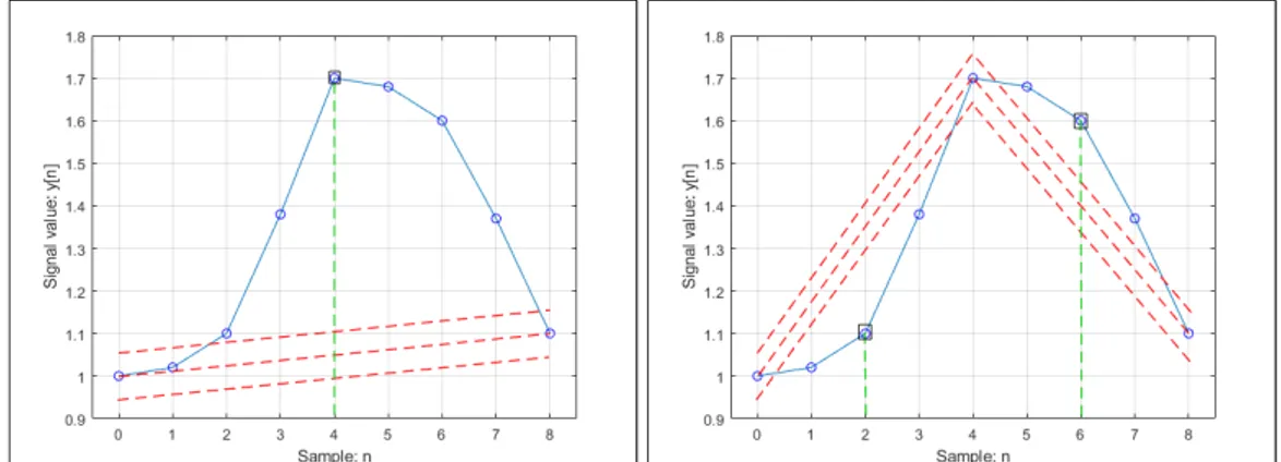
Here we give a step-by-step demonstration of the fractal resampling compression, on a sequence of a nine sample data. Each sample is denoted as a pair of (x,y) coordinates, usually generated with an equal inter-arrival period. Note that blue lines represent original signal, whereas red dashed lines define region of tolerance for midpoint check. In the first step we draw a line between the first and the last point in the sequence, which are stored by default. Next we define an error tolerance region, bounded with upper and lower line, and check whether the midpoint belongs to the region. If it is inside, then the point is discarded, otherwise it must be stored and used in the process of signal reconstruction (decoding). The point splits the sequence into two sub-sequences (see figure 8.2. The same process is performed on each next sub-level. Third (last) level for a sequence of eight samples is presented on the figure 8.3. There are log2N steps in total, for N samples in the data set,

where N is selected as 2n+ 17.

The reconstructed signal is completely composed of the samples contained in the time-sequence original. In this example, reconstructed signal is a time-series of x(0), x(2), x(4), x(6) and x(8). Calculated CR value, according to 7.1.2, is 45.5 %.

The core problematics of the research revolves around the compression ratio accomplished on battery data, particularly on current, voltage and temperature signals.

8.3 Critical Aperture - CA

Critical Aperture compression is based on slope calculation, and it is also known as ”rate of change” compression. The method is based on slope calculation and strives to eliminate all the points situated within a certain slope boundary. The following example briefly describes the algorithm. There we have a sequence of eight samples, with an approximate slope error tolerance represented by vertical double-arrow.

6_{n is a natural number (positive integer, i.e. 0,1,2,3...)} 7_{n is an integer number greater than zero}

(31)

Figure 8.1: The first midpoint, arith-metic mean of the first and the last point in the sequence: x(4)

Figure 8.2: Sequence divided into two sub-sequences, arithmetic means at x(2) and x(6)

Figure 8.3: Arithmetic means at x(1), x(3), x(5) and x(7)

Figure 8.4: Signal plot of the original and compressed data

At the start, we define an initial slope value by use of x(0) and x(1). Next, it is necessary to fence allowed slope region, with regard to error tolerance. Initial slope field is marked with black straight lines A.19. Sample x(2) is the first to be tested, and slope of the point is lying within black boundaries, and the sample is discarded. In the next step, we take a look at the sample x(3) and mark the margins with respect to point x(2), represented by red region. Naturally, point x(3) is enclosed by red margins and therefore discarded for future use. Applying the same procedure on point x(4), represented by green lines, we see that the sample is out and therefore x(3) is stored as the last reference point.

In the next phase, we generate the reference slope using the points x(3) and x(4) expecting the x(5) lie in between black region, as shown on figure A.20. However, the point is out, and its predecessor x(4) is stored as a temporary reference. Going for the sample with index 6, and checking its affiliation for the black region, we see that it is not necessary to store the point. Eventually, the last sample, x(7), does not belong to the red region and therefore is stored in the sequence of compressing data (see figure 8.7). On the last graph, shown in figure 8.8, we see the comparison of the original data, represented by a blue and the compressed data depicted by a red plot.

(32)

Figure 8.5: Initial slope with x(0) and x(1), further points x(2), x(3) and x(4) - x(3) stored

Figure 8.6: Slope generated with x(3) and x(4). Unsuccessful check at point x(5) - x(4) stored

Figure 8.7: Referent slope with with x(4) and x(5) - x(6) stored

Figure 8.8: Original and compressed signal on the same plot

8.4 Fast Fourier Transform - FFT

FFT algorithm is mainly based on grouping (dividing) of the data-set into two subsets. Each subset is further halved until all the samples are distributed into pairs (see figure 8.9). Conventional DFT is applied on each pair as shown by the formula 8.4.1 X3(m) = x(0) + W2mx(1) (8.4.1) X3(0) = x(0) + x(1), W20 = e 2π 2 0 = 1 (8.4.2) X3(1) = x(0) − x(1), W21 = e 2π 2 1 = −1 (8.4.3)

Going a step back we calculate X2(m) and X1(m)8.

Backward process is depicted on the figure 8.10

For a data set of N samples, there are log2N steps of decomposition. Each

step requires N complex summations and N/2 complex multiplications. Hence, the algorithm complexity is represented as N log2N . Size of the data in the compressed

form is halved, since the frequency spectrum of the signal is symmetric, as a result of existing complex conjugates.

(33)

Figure 8.9: Data split process from the initial data set to the pairs

Figure 8.10: Backward calculation of the coefficients on sub-levels. Cooley-Tukey FFT with time decimation for N=8

8.5 Discrete Cosine Transform - DCT

DCT algorithm is based on similar calculation arithmetics as DFT. However, DFT considers an original time domain sequence to be in complex form, mapping it to corresponding complex form in the frequency domain. If a target signal is entirely in the time domain, then DFT execution complexity would be reduced, but still obtaining many unnecessary computations. In IoT sensory data acquisition, the data is always real. Hence applying DCT on the signal would result in the only real spectrum of coefficients. The algorithm can also be applied in ”fast” form, similarly as FFT. For this implementation, the model of Fast Discrete Cosine Transform pro-posed by Lee (MIT) took place [30]. Here we present some of the DCT forms: DCT-I Xk= 1 2(x0+ (−1) k_X N −1) + N −2 X n=1 xncos[ π N − 1nk] (8.5.1) DCT-II Xk = N −1 X n=0 xncos[ π N(n + 1 2)k] (8.5.2) DCT-III Xk = 1 2x0+ N −1 X n=1 xncos[ π N(n + 1 2)] (8.5.3)

(34)

DCT-IV Xk = N −1 X n=0 xncos[ π N(n + 1 2)(k + 1 2)] (8.5.4)

For a decompression process, it is necessary to obtain inverse transform, which slightly differs for all of the direct forms. Inverse transform of any formula is quite similar to the direct one. Hence:

Inv(DCT − I) = 2 N − 1DCT − I (8.5.5) Inv(DCT − II) = 2 NDCT − III (8.5.6) Inv(DCT − III) = 2 NDCT − II (8.5.7) Inv(DCT − IV ) = 2 NDCT − IV (8.5.8)

(35)

9 System setup

To be able to test compression algorithms, and to answer the research questions asked in this thesis, some kind of hardware was necessary to do the evaluation. De-velopment board EVK1100 with Atmels AT32UC3A0512 32 Bit microcontroller and FreeRTOS embedded operating system running on it, was used in conjunction with Sodaq Explorer development board with 32-Bit ARMs M0+ cortex ATSAMD21J18. Algorithms that were chosen in chapter 6 were implemented on EVK1100 board in Atmel Studio 7 IDE and programmed with Atmel’s AVR Dragon debugger trough JTAG. The algorithms were first tested and implemented in MATLAB. Afterward, they are mapped into corresponding C code and downloaded to the board. Sodaq Explorer board was connected via USART with EVK1100 board. Compressed data is sent to the cloud via Sodaqs LoRa IoT module, which is part of Explorer board. Data is sent via LoRa wireless protocol from the end node to the router gateway.

Gateway hardware is Lairds Senturius RG186. Ethernet that was connected to the things network [31]. The gateway was registered by following the instructions after creating an account on the website mentioned above. Sodaq board, which is Arduino compatible, was programmed with instructions from official Sodaq support website [32], with some minor changes to the provided sketch program. Thus, it can be connected to EVK1100 board and assigned to Things Network as an application.

Entire system is presented on the figure 9.1

9.1 Implementation

Implementation of the algorithms is initially performed in MATLAB, where data han-dling is much faster and easier. After the testing is completed algorithm is down-loaded to EVK1100 board. The detailed implementation of selected algorithms is described in Application section.

Testing points were put in MCU internal flash memory and stored as an array of type double, with actual values. However, there is an exception to FFT, which need a special data treatment. It is first mapped to range [−1, 1] and then using macro converted from float type to signed fixed-point Q1.31 type, that is optimized for FFT and other DSP functions.

FFT compression algorithm is implemented with DSP library from Atmel Studio IDE, which contains a hardware-specific integrated example. This means that the algorithm for determining FFT coefficients has been optimized by writing a majority of the code in assembly language. Code optimization also includes a look-up table for twiddle factors, for up to 1024 coefficients. This makes the calculation process faster. FFT function requires three parameters: a vector for coefficients storing, an input vector, and a parameter that defines log2(Size) where Size is a number of

samples for the data set. The function requires all the data points to be stored before a function call. This implies that the function does not exhibit RT capabilities. The compression process is performed by calculating the absolute value of a complex number, to determine the spectral coefficients. The error bound is defined after determining the range between the maximum and minimum value of the coefficients. Coefficients are removed from the final array and set to zero if they are smaller than

BATTERY SENSORY DATA COMPRESSION FOR ULTRANARROW BANDWIDTH IOT PROTOCOLS